phase diagram of the one dimensional $S=\frac{1}{2}$ $XXZ$ model with Ferromagnetic nearest-neighbor and Antiferromagnetic next-nearest neighbor interactions

Abstract

We have studied the phase diagram of the one dimensional $S=\frac{1}{2}$ $XXZ$ model with ferromagnetic nearest-neighbor and antiferromagnetic next-nearest neighbor interactions. We have applied the quantum renormalization group (QRG) approach to get the stable fixed points and the running of coupling constants. The second order QRG has been implemented to get the self similar Hamiltonian. This model shows a rich phase diagram which consists of different phases which possess the quantum spin-fluid and dimer phases in addition to the classical Néel and ferromagnetic ones. The border between different phases has been shown as a projection onto two different planes in the phase space.

I Introduction

There is currently much interest in quantum spin systems that exhibit frustrations. This has been simulated in particular by study of the magnetic properties of the cuprates which become high- $T_{c}$ superconductors when doped. Frustrated spin systems are known to have many interesting properties which are quite different from the conventional magnetic systems.

The Heisenberg spin $\frac{1}{2}$ chain with nearest neighbor (NN) and next-nearest neighbor (NNN) interactions (which is equivalent to a zig-zag ladder) is a typical model with frustrations. In the recent years, several interesting quasi-one-dimensional magnetic systems have been studied experimentally Hase ; Motoyama ; Coldea . Among them, some compounds containing $CuO$ chains with edge-sharing $CuO_{4}$ plaquette were expected to be described by the $XXZ$ model with next-nearest neighbor interactions. The nearest-neighbor $(Cu-Cu)$ spin interaction changes from antiferromagnetic (AFM) to ferromagnetic (FM), as the angle $\theta$ of the $Cu-O-Cu$ bound approaches $90^{o}$. The next-nearest-neighbor interaction is always AFM and is not dependent on $\theta$ Mizuno . Several compounds with edge- sharing chains are known, such as $Li_{2}CuO_{2}$, $La_{6}Ca_{8}Cu_{21}O_{41}$, $Ca_{2}Y_{2}Cu_{5}O_{10}$, $Rb_{2}Cu_{2}Mo_{3}O_{12}$, which can be considered as an ideal model compounds with the ferromagnetic NN interactions and antiferromagnetic NNN interactions solodovnikov ; Hase-Kuroe .

The Hamiltonian of such model on a periodic chain of $N$ sites is

$$H=\frac{J}{4}\big{\{}\sum_{i=1}^{N}(\sigma_{i}^{x}\sigma_{i+1}^{x}+\sigma_{i}^{y}\sigma_{i+1}^{y}+\Delta~{}\sigma_{i}^{z}\sigma_{i+1}^{z})+\sum_{i=1}^{N}J_{2}(\sigma_{i}^{x}\sigma_{i+2}^{x}+\sigma_{i}^{y}\sigma_{i+2}^{y}+\delta~{}\sigma_{i}^{z}\sigma_{i+2}^{z})\big{\}},$$ (1)

where $J>0$ and $J_{2}\geq 0$ are the first and second-nearest neighbor exchange couplings and the corresponding easy-axis anisotropies are defined by $\Delta$ and $\Delta_{2}=J_{2}\delta$. For $J_{2}=0$, the ground state properties are well known from the Bethe ansatz Cloizeaux . For positive coupling constants ($J,J_{2},\Delta,\delta>0$), this model has been investigated previously Nomura ; Langari . In particular, it has been shown that a transition from a gapless state to a dimerized one takes place at $(J_{2}=0.24,\Delta=\delta=1)$ Nomura2 . The point $(J_{2}=\frac{1}{2},\Delta=\delta=1)$ corresponds to the well known Majumdar-Ghosh model where the exact ground state is constructed from the direct products of dimers which leads to a gapful phase Majumdar . Relatively, less is known about the model with the ferromagnetic NN and the antiferromagnetic NNN interactins. Though the latter model has been a subject of many studies Bursill ; Tonegawa ; Cabra ; Krivnov , the complete picture of the phases in this model is still in investigation Dmitriev . It is well known that there is a critical point $(J_{2}=\frac{1}{4},\Delta=-\delta=-1)$ where the ferromagnetic state is unstable and the ground state is nontrivial at $J_{2}>\frac{1}{4}$ which can be realized by different phases Chubukov . Moreover, the exact ground state can be represented in the resonating valence bound state (RVB) Bader ; Hamada . This state has been proposed as a candidate for the spin liquid ground state Anderson . One of the most important and open question is the possibility of the spontaneous dimerization of the system in the singlet phase accompanying by a gap in the spectrum Dmitriev2 . The controversial conclusion exists about the presence of a gap at $J_{2}>\frac{1}{4}$. It has long been believed that the model is gapless White ; Allen but one loop renormalization group analysis shows Cabra ; Nersesyan that the gap opens due to a Lorentz symmetry breaking perturbation. However, the gap has not been checked numerically Cabra . On the base of field theory consideration it was proposed Itoi that a very tiny but finite gap exists which can not be observed numerically.

In this paper we have considered the one dimensional anisotropic $S=\frac{1}{2}$ Heisenberg model with ferromagnetic NN and antiferromagnetic NNN interactions by implementing the quantum renormalization group (QRG) method. We have calculated the effective Hamiltonian up to the second order corrections. The second order correction is necessary to get a self similar Hamiltonian after each step of QRG. In this approach, we have considered the effect of whole states of the block Hamiltonian which are partially ignored in the first order approach. The present scheme allows us to have the analytic RG equations, which give a better understanding of the behavior of system by running of coupling constants. We have succeeded in obtaining the phase diagram in a good qualitative agreement with the numerical ones Somma .

We have previously studied the antiferromagnetic model (Eq.(1)) for $\Delta>0$ by QRG Langari . For $0\leq\Delta<1$ the interplay of the two competing terms (NN and NNN) in the presence of quantum fluctuations produces the dimer phase for $J_{2}\geq J_{2}^{c}(\Delta,\Delta_{2})$. The dimer or spin Peierls phase has a spin gap and a broken translation symmetry (the unit cell is doubled) in the thermodynamic limit. However, we have determined the fluid-dimer phase transition by using the running of couplings under RG (see Fig.3 of Ref.Langari or the complete phase diagram presented in Fig.3 in this article). In the spin-fluid phase, the anisotropy and next-nearest neighbor couplings are irrelevant while in the dimer phase they run to the triple point ($\Delta_{2}^{*}=J_{2}^{*}\simeq 0.155,\Delta^{*}=1$). From a quantitative point of view at $\Delta=0$ the RG analysis gives $J_{2}^{c}\simeq 0.44$ which can be compared with the numerical result of $J_{2}^{c}\simeq 0.33$ presented in Ref.Nomura . The Néel phase appears just by crossing the $\Delta=1$ plane at $\Delta_{2}=0$ and $J_{2}=0$. In the $\Delta_{2}=0$ plane and for $\Delta>1$, the model will pass through a phase transition from Néel to dimer phase for $J_{2}>J_{2}^{c}(\Delta)$. The Néel ordered is also broken by increasing the anisotropy of the NNN interaction.

In this paper we will complete the phase diagram of this model for the whole range of parameters. Moreover, we intend to consider the $XXZ$ model with ferromagnetic NN ($J<0$) and antiferromagnetic NNN ($JJ_{2}>0$) interactions which can be fulfilled by extending the phase diagram to $J<0$ and $JJ_{2}>0$. If we implement a $\pi$ rotation around $z$ axis for the even sites and leave the odd sites unchanged, the Hamiltonian (with $J<0$ and $JJ_{2}>0$) is transformed to the following from

$$H=\frac{J}{4}\big{\{}\sum_{i=1}^{N}(\sigma_{i}^{x}\sigma_{i+1}^{x}+\sigma_{i}^{y}\sigma_{i+1}^{y}-\Delta~{}\sigma_{i}^{z}\sigma_{i+1}^{z})+\sum_{i=1}^{N}J_{2}(\sigma_{i}^{x}\sigma_{i+2}^{x}+\sigma_{i}^{y}\sigma_{i+2}^{y}+\delta~{}\sigma_{i}^{z}\sigma_{i+2}^{z})\big{\}};~{}~{}~{}J,J_{2},\Delta,\delta>0.$$ (2)

The QRG procedure is implemented on the rotated Hamiltonian (Eq.(2)) which makes the calculations easier. However, the phase diagram and other figures presented in this article are based on the couplings defined in Eq.(1).

The QRG approach will be explained in the next section where the second order effective Hamiltonian and the renormalization of the coupling constants are obtained. In Sec. III , We will present the phase diagram and its characteristics where a comparison with numerical results is done Somma . Finally, we summarize our results.

II RG equations

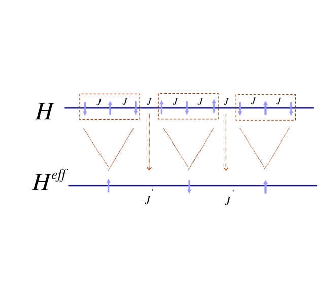
Figure 1: The decomposition of chain into three site blocks Hamiltonian ($H^{B}$) and inter-block Hamiltonian ($H^{BB}$).

The main idea of the QRG method is the mode elimination or thinning of the degrees of freedom followed by an iteration which reduces the number of variables step by step until a more manageable situation is reached. We have implemented the Kadanoff’s block method to do this purpose, because it is well suited to perform analytical calculation in the lattice models and they are conceptually easy to be extended to the higher dimensions. In Kadanoff’s method, the lattice is divided into blocks where the Hamiltonian is exactly diagonalized. By selecting a number of low-lying eigenstates of the blocks the full Hamiltonian is projected into these eigenstates which gives the effective (renormalized) Hamiltonian. The effective Hamiltonian up to second order corrections is Langari ; miguel1 ; miguel-2

$$H^{eff}=H^{eff}_{0}+H^{eff}_{1}+H^{eff}_{2}.$$

$$H^{eff}_{0}=P_{0}H^{B}P_{0}~{}~{}~{},~{}~{}~{}H_{1}^{eff}=P_{0}H^{BB}P_{0}~{}~{}~{},~{}~{}~{}H_{2}^{eff}=P_{0}[H^{BB}(1-P_{0})\frac{1}{E_{0}-H^{B}}(1-P_{0})H^{BB}]P_{0}.$$

We have applied the mentioned scheme to the Hamiltonian defined in Eq.(2). We have considered three-site block procedure defined in Fig.(1). The block Hamiltonian ($H^{B}=\sum h_{I}^{B}$) of the three sites, its eigenstates and eigenvalues are given in appendix A. The three site block Hamiltonian has four doubly degenerate eigenvalues (see appendix A). $P_{0}$ is the projection operator to the ground state subspace which defines the RG procedure. Due to the level crossing which occurs for the eigenstates of the block Hamiltonian, the projection operator ($P_{0}$) can be different depending on the coupling constants. Therefore, we must specify the regions with the corresponding ground states. The eigenvalues of the block Hamiltonian are labeled by $e_{0},e_{1},e_{2},e_{3}$ (see appendix A). In the following, we will classify the regions where each of this states represent the ground state. A summary of this information is given in Fig.(4) of appendix A.

II.1 Region (A): $e_{0}$ is the ground state.

In this region the effective Hamiltonian in the first order correction leads to the $XXZ$ chain without the NNN interaction ($J^{\prime}_{2}=0$), i.e the effective Hamiltonian is not exactly similar to the initial one. The NNN interaction is the result of the second order correction. When the second order correction is added to the effective Hamiltonian, the renormalized Hamiltonian, apart from an additive constant, is similar to Eq.(2) with the renormalized couplings. Thus, the effective Hamiltonian including the second order correction for $\Delta>0$ is:

$$H^{eff}=\frac{J^{\prime}}{4}\left[\sum_{i}^{N/3}({\sigma}_{i}^{x}{\sigma}_{i+1}^{x}+{\sigma}_{i}^{y}{\sigma}_{i+1}^{y})-\Delta^{\prime}({\sigma}_{i}^{z}{\sigma}_{i+1}^{z})+\sum_{i}^{N/3}J_{2}^{\prime}({\sigma}_{i}^{x}{\sigma}_{i+2}^{x}+{\sigma}_{i}^{y}{\sigma}_{i+2}^{y})+\Delta_{2}^{\prime}({\sigma}_{i}^{z}{\sigma}_{i+2}^{z})\right].$$

The renormalized coupling constants are functions of the original ones which are given in appendix B.

II.2 Region (B): $e_{2}$ is the ground state.

The second order effective Hamiltonian is similar to the case of region A with different coupling constants given in appendix C. A note is in order here, although the second order correction is necessary to produce the NNN interaction in the effective Hamiltonian the initial values of $J_{2}=0$ and $\Delta_{2}=0$ do not produce NNN interactions. It is different from the RG flow obtained in region A.

II.3 Region (C): $e_{3}$ is the ground state.

In this region the effective Hamiltonian to the second order corrections leads to the Ising model

$$H^{eff}=\frac{1}{4}\left[\sum_{i}^{N/3}-\Delta^{\prime}({\sigma}_{i}^{z}{\sigma}_{i+1}^{z})\right].$$

Where

$$\Delta^{\prime} = J(\Delta+2\Delta_{2})$$

$$+ \frac{J^{2}}{4}\left[(\frac{1}{e_{3}-e_{0}})(\frac{1}{2+q^{2}})(1+2J_{2}q)^{2}+(\frac{1}{e_{3}-e_{1}})(\frac{1}{2+p^{2}})(1+2J_{2}p)^{2}+(\frac{1}{e_{3}-e_{2}})(\frac{1}{2})^{2}\right]$$

$$+ J^{2}\left[(\frac{1}{2e_{3}-e_{1}-e_{0}})(\frac{1}{2+q^{2}})(\frac{1}{2+p^{2}})(1+2J_{2}(p+q))^{2}+(\frac{1}{2e_{3}-e_{2}-e_{0}})(\frac{1}{2+q^{2}})(\frac{1}{2})(1+2J_{2}q)^{2}\right.$$

$$+ \left.(\frac{1}{2e_{3}-e_{2}-e_{1}})(\frac{1}{2+p^{2}})(\frac{1}{2})(1+2J_{2}p)^{2}\right].$$

This simply introduces the ferromagnetic behavior. We will discuss the phase diagram in terms of different regions defined above in the following section.

III Phase diagram

III.1 Region (A)

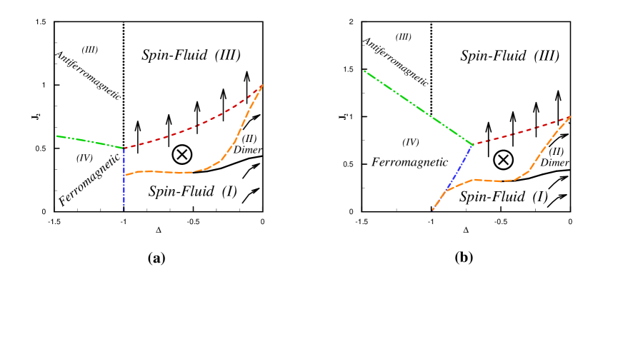
Figure 2: The cross section of the three dimensional phase diagram for $\Delta<0$. (a) The crossed plane is $\Delta_{2}=J_{2}\Delta$ and (b) $\Delta_{2}=0$.

In the $\Delta<0$ case, the RG equation shows running of $J$ to zero which represents the renormalization of the energy scale. We have plotted the RG flow and different phases in Fig.(2). The solid line is the boundary between dimer (II) phase and spin-fluid (I) phase. If we start from the spin -fluid (I) phase or Dimer (II) phase, the sign of NN anisotropy ($\Delta$) changes under RG after few steps. However, in the dimer (II) phase the amount of NNN coupling ($J_{2}$) is greater than 0.44 just when the anisotropy changes sign, while in the spin-fluid (I) phase it is less than 0.44. In other words, in dimer (II) phase the RG flow goes to the triple point ($\Delta_{2}^{*}=J_{2}^{*}\simeq 0.155,\Delta^{*}=1$) (the filled circle in Fig.(3)) while it goes to $\Delta=J_{2}=\Delta_{2}=0$ fixed point starting from the spin-fluid (I) phase. In Fig.(2(a)) and Fig.(2(b)) the black arrows show the running of couplings under RG. In the region denoted by $\bigotimes$, though $e_{0}$ is the ground state, the behavior of the couplings constant is not the same as the couplings in the dimer (II) phase. In this region ($\bigotimes$) coupling constants go to the spin-fluid (III) phase. It means that the region denoted by $\bigotimes$ and spin-fluid (III) are a unique phase. The authors in the reference Somma were not able to specify the phase of this region numerically. We denote the boundary between the spin-fluid (III) and both dimer (II) and spin-fluid (I) phases by long-dashed line. The dashed line behind the arrows is not a phase boundary and just represents the two regions with differenet ground states (see appendix A). It is known that on the $\Delta_{2}=J_{2}\Delta$ plane and $\Delta=-1$ there is a fixed point, namely: $\Delta=-1,J_{2}=0.25$ Bader ; Hamada . However, our approach is not able to show this fixed point because this is on the plane which is separated by spin-fluid (I) and ferromagnetic phases where the level crossing occurs. Instead, close to the $\Delta=-1$ line we found the critical value of $J_{2}^{c}=0.28$ which distinguishes the spin-fluid (I) and spin-fluid (III) phases.

III.2 Region (B)

In this region the NNN interactions are greater than NN interactions. The implementation of bosonization technique combined with a meanfield analysis in the reference Nersesyan predicted that for $\Delta_{2}=J_{2}\Delta$ plane and $\Delta=0$, the system might exhibit a chiral ordered phase with gapless excitations where $J_{2}>J_{2}^{c}=1.26$. The predicted critical value ($J_{2}^{c}$) is in well agreement with the numerical density matrix renormalization group result Hikihara . Our approach shows that all coupling constants are irrelevant except $J_{2}$ and $\Delta_{2}$. For $-1<\Delta<0$ the ratio of $\Delta_{2}$ to $J_{2}$ goes to zero and for $\Delta<-1$ this ratio goes to infinity. It means that in the fixed point of this region the original spin chain decouples to two $XXZ$ chains without next-nearest-neighbor interactions where the lattice spacing is doubled. For $-1<\Delta<0$, the model is in the spin-fluid (III) phase which is specified in Fig.(2). The spin-fluid (III) is different from the spin-fluid (I) phase according to their stable fixed points. The stable fixed point for spin-fluid (I) is $J_{2}=0,\Delta_{2}=0$ while for spin-fluid (III) it is $\frac{\Delta_{2}}{J_{2}}\rightarrow 0$ having $J_{2},\Delta_{2}\rightarrow\infty$. Note that the level crossing of $e_{0}$ and $e_{2}$ does not define the border between spin-fluid (III) and dimer (II) phase. This border is defined by the running of couplings under RG equations. For $\Delta<-1$ the model is in the antiferromagnetic phase. In this case the model is decoupled to two antiferromagnetic Ising chains. Thus the ground state is long-ranged antiferromagnetic ordered $|\uparrow\uparrow\downarrow\downarrow\uparrow\uparrow\downarrow\downarrow\cdots\rangle$.

III.3 Region (C)

As we pointed out in sec.II-C, even after adding the second order corrections, the original Hamiltonian is mapped to the ferromagnetic Ising model. Ising model remains unchanged under RG as fixed point and its properties are well known. We call this region as the ferromagnetic phase.

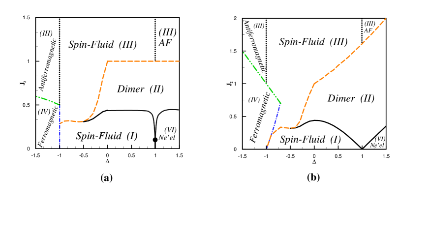
Figure 3: The projection of the complete phase diagram on the $\Delta{2}=J_{2}\Delta$ plane in (a) and on the $\Delta_{2}=0$ plane in (b).

IV Summary and discussions

We mapped the one dimensional ferromagnetic NN and antiferromagnetic NNN $S=\frac{1}{2}$ $XXZ$ model to the antiferromagnetic model in Eq.(2) with negative anisotropy. We have implemented the second order QRG procedure to get the phase diagram of this model. The complete phase diagram which also covers the positive anisotropy region is presented in Fig.(3). This is a cross section of the phase diagram with $\Delta_{2}=J_{2}\Delta$ plane in Fig.3(a) and with $\Delta_{2}=0$ plane in Fig.3(b). For $-0.5<\Delta<1$ (on $\Delta_{2}=J_{2}\Delta$ plane), when $J_{2}$ is smaller than the critical value ($J_{2}^{c}$) the system is in the gapless spin-fluid (I) phase. By contrast, for larger value of $J_{2}>J_{2}^{c}$ the system is in the dimer phase with a finite energy gap above the doubly degenerate ground states (the transition is denoted by solid line). As $J_{2}$ increases, the system exhibits a transition from the dimer phase to the spin-fluid (III) phase which is called the gapless chiral phase in Ref.Hikihara . The transition is denoted by long dashed line on the phase diagram. The transition takes place at $J_{2}^{c}=1$ for $\Delta=0$, in qualitative agreement with $J_{2}^{c}=1.26$ of Ref.Hikihara . For $-1<\Delta<-0.5$ (On the $\Delta_{2}=J_{2}\Delta$ plane) at $J_{2}^{c}$ a transition occurs from the spin-fluid(I) to spin-fluid (III) (chiral order) phases. The QRG equations for $\Delta\gtrsim-1$ shows a critical line (long dashed line) which separates the spin-fluid (I) and spin-fluid (III) phases without an intermediate region. Thus, we claim that for $J_{2}>J_{2}^{c}=0.28$ there is no gap and the model is not in the dimer phase. The model is in ferromagnetic phase where $\Delta<-1$ and small $J_{2}$. The phase transition to long-range antiferremagnetic phase takes place at $J_{2}>J_{2}^{c}$ (dashed-dot-dot line). In the case of $\Delta>1$, a transition from Néel (VI) phase to the dimer phase occurs as $J_{2}$ increases (solid line). The dimer phase is unstable by increasing $J_{2}$ further which leads to a transition to the antiferromagnetic (AF(III)) phase (long dashed line). However, The comparison of Fig.3(a) with Fig.3(b) shows that the anisotropy of the NNN-term ($\Delta_{2}$) changes the phase diagram significantly. From the parameters estimated for several compounds near the isotropic limit ($\Delta=1,\Delta_{2}=J_{2}\Delta$), $La_{6}Ca_{8}Cu_{21}O_{41}$ ($J_{2}^{c}=0.36$), $Li_{2}CuO_{2}$ ($J_{2}^{c}=0.62$), $Ca_{2}Y_{2}Cu_{5}O_{10}$ ($J_{2}^{c}=2.2$) Mizuno , our result predict for $\Delta>-1$ that all of them are in the chiral order phase (spin-fluid(III)) without gap, and for $\Delta<-1$, $La_{6}Ca_{8}Cu_{21}O_{41}$ is in the ferromagnetic phase and $Li_{2}CuO_{2}$, $Ca_{2}Y_{2}Cu_{5}O_{10}$ are in long-range antiferromagnetic order.

V acknowledgment

The authors would like to thank Prof. M. R. H. Khajehpour for careful reading of the manuscript and fruitful discussions.

Appendix A The block Hamiltonian of three sites, its eigenvectors and eigenvalues

We have considered the three-site block (Fig.(1)) with the following Hamiltonian

$$h_{I}^{B}=\frac{J}{4} [(\sigma_{1,I}^{x}\sigma_{2,I}^{x}+\sigma_{2,I}^{x}\sigma_{3,I}^{x}+\sigma_{1,I}^{y}\sigma_{2,I}^{y}+\sigma_{2,I}^{y}\sigma_{3,I}^{y})-\Delta(\sigma_{1,I}^{z}\sigma_{2,I}^{z}+\sigma_{2,I}^{z}\sigma_{3,I}^{z})$$

$$+J_{2}(\sigma_{1,I}^{x}\sigma_{3,I}^{x}+\sigma_{1,I}^{y}\sigma_{3,I}^{y})+\Delta_{2}(\sigma_{1,I}^{z}\sigma_{3,I}^{z})],$$

where $\sigma_{j,I}^{\alpha}$ refers to the $\alpha$-component of the Pauli matrix at site $j$ of the block labeled by $I$. The exact treatment of this Hamiltonian leads to four distinct eigenvalues which are doubly degenerate. The ground, first, second and third excited state energies have the following expressions in terms of the coupling constants.

$$|\psi_{0}\rangle=\frac{1}{\sqrt{2+q^{2}}}(|\uparrow\uparrow\downarrow\rangle+q|\uparrow\downarrow\uparrow\rangle+|\downarrow\uparrow\uparrow\rangle)~{}~{}~{},~{}~{}~{}|\psi_{0}^{\prime}\rangle=\frac{1}{\sqrt{2+q^{2}}}(|\uparrow\downarrow\downarrow\rangle+q|\downarrow\uparrow\downarrow\rangle+|\downarrow\downarrow\uparrow\rangle),$$

$$e_{0}=\frac{J}{4}[~{}J_{2}+\Delta-\sqrt{{(J_{2}-\Delta-\Delta_{2})}^{2}+8}],~{}~{}~{}~{}~{}~{}~{}~{}~{}~{}~{}~{}~{}~{}~{}~{}~{}~{}~{}~{}~{}~{}~{}~{}~{}~{}~{}~{}~{}$$

$$|\psi_{1}\rangle=\frac{1}{\sqrt{2+p^{2}}}(|\uparrow\uparrow\downarrow\rangle+p|\uparrow\downarrow\uparrow\rangle+|\downarrow\uparrow\uparrow\rangle)~{}~{}~{},~{}~{}~{}|\psi_{1}^{\prime}\rangle=\frac{1}{\sqrt{2+p^{2}}}(|\uparrow\downarrow\downarrow\rangle+p|\downarrow\uparrow\downarrow\rangle+|\downarrow\downarrow\uparrow\rangle),$$

$$e_{1}=\frac{J}{4}[~{}J_{2}+\Delta+\sqrt{{(J_{2}-\Delta-\Delta_{2})}^{2}+8}],~{}~{}~{}~{}~{}~{}~{}~{}~{}~{}~{}~{}~{}~{}~{}~{}~{}~{}~{}~{}~{}~{}~{}~{}~{}~{}~{}~{}~{}$$

$$|\psi_{2}\rangle=\frac{1}{\sqrt{2}}(|\downarrow\downarrow\uparrow\rangle-|\uparrow\downarrow\downarrow\rangle)~{}~{}~{},~{}~{}~{}|\psi_{2}^{\prime}\rangle=\frac{1}{\sqrt{2}}(|\uparrow\uparrow\downarrow\rangle-|\downarrow\uparrow\uparrow\rangle),$$

$$e_{2}=\frac{-J}{4}(~{}2J_{2}+\Delta_{2}),~{}~{}~{}~{}~{}~{}~{}~{}~{}~{}~{}~{}~{}~{}~{}~{}~{}~{}~{}~{}~{}~{}~{}~{}~{}$$

$$|\psi_{3}\rangle=|\uparrow\uparrow\uparrow\rangle~{}~{}~{},~{}~{}~{}|\psi_{3}^{\prime}\rangle=|\downarrow\downarrow\downarrow\rangle,$$

$$e_{3}=\frac{J}{4}(\Delta_{2}-2\Delta),~{}~{}~{}~{}~{}~{}~{}~{}~{}$$

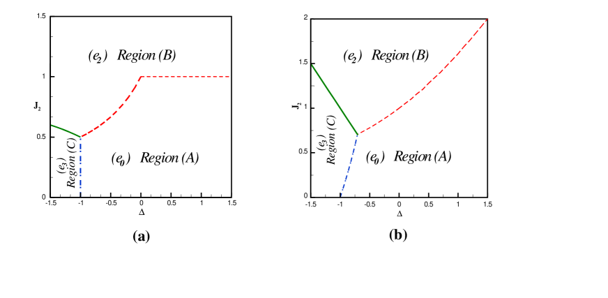
Figure 4: The projection of the three dimensional border areas on the $\Delta{2}=J_{2}\Delta$ plane (a) and for $\Delta_{2}=0$ plane in (b).

where $q,p$ are

$$q=\frac{-1}{2}[J_{2}-\Delta-\Delta_{2}+\sqrt{{(J_{2}-\Delta-\Delta_{2})}^{2}+8}]~{}~{}~{},~{}~{}~{}p=\frac{-1}{2}[J_{2}-\Delta-\Delta_{2}-\sqrt{{(J_{2}-\Delta-\Delta_{2})}^{2}+8}].$$

$|\uparrow\rangle$ and $|\downarrow\rangle$ are the eigenstates of $\sigma^{z}$.

In Fig.(4) we have presented the different regions where the specified state is the ground state of the block Hamiltonian. The border between these regions are specified as a projection to a fixed plane. The projection to $\Delta_{2}=J_{2}\Delta~{}(\Delta=\delta)$ plane is shown in Fig.4(a) and the projection to $\Delta_{2}=0$ plane is plotted in Fig.4(b).

Appendix B The renormalized coupling constants of the effective Hamiltonian in region A

$$J^{\prime} = J(\frac{2}{2+q^{2}})^{2}(q^{2}+2J_{2}q)+\frac{J^{2}}{4}(\frac{\Delta}{e_{0}-e_{2}})(\frac{q}{2+q^{2}})^{2}$$

$$- \frac{J^{2}}{4}(\frac{1}{e_{0}-e_{1}})(\frac{1}{(2+q^{2})(2+p^{2})})^{2}(p+q)(pq)(p+q+4J_{2})(4\Delta_{2}-(\Delta+2\Delta_{2})pq)$$

$$- \frac{J^{2}}{4}(\frac{4}{2e_{0}-e_{1}-e_{2}})(\frac{1}{2+q^{2}})^{2}(\frac{q}{2+p^{2}})(p+q+2J_{2})(2\Delta_{2}-(\Delta+\Delta_{2})pq).$$

$$\Delta^{\prime} = \left\{J(\frac{q}{2+q^{2}})^{2}(\Delta q^{2}-2\Delta_{2}(2-q^{2}))+\frac{J^{2}}{4}(\frac{1}{e_{0}-e_{1}})(\frac{(p+q)^{2}+4J_{2}(p+q)}{(2+q^{2})(2+p^{2})})^{2}\right.$$

$$+ \frac{J^{2}}{4}(\frac{1}{e_{0}-e_{2}})(\frac{q^{2}}{2(2+q^{2})})^{2}+\frac{J^{2}}{4}(\frac{1}{e_{0}-e_{3}})(\frac{1+2J_{2}q}{2+q^{2}})^{2}$$

$$+ \frac{J^{2}}{4}(\frac{2}{2e_{0}-e_{1}-e_{2}})(\frac{1}{2+p^{2}})(\frac{q(~{}p+q+2J_{2})}{2+q^{2}})^{2}-\frac{J^{2}}{4}(\frac{2}{2e_{0}-e_{2}-e_{3}})(\frac{q(1+qJ_{2})}{2+q^{2}})^{2}$$

$$- \left.\frac{J^{2}}{4}(\frac{4}{2e_{0}-e_{1}-e_{3}})(\frac{J_{2}(pq+q^{2}+2)+p+q}{(2+q^{2})(2+p^{2})^{1/2}})^{2}\right\}/J^{\prime}.$$

$$J^{\prime}_{2}=\left\{\frac{J^{2}}{4}(\frac{2}{2+q^{2}})^{3}\left[\frac{(J_{2}(3q+p)+q(p+q))^{2}}{(e_{0}-e_{1})(2+p^{2})}+\frac{(J_{2}(1+q^{2})+q)^{2}}{e_{0}-e_{3}}-\frac{(q^{2}+J_{2}q)^{2}}{2(e_{0}-e_{2})}\right]\right\}/J^{\prime}.$$

$$\Delta^{\prime}_{2}=\left\{\frac{J^{2}}{4}(\frac{2}{2+q^{2}})^{3}\left[\frac{(\Delta_{2}q(p-pq^{2}+q)-\frac{\Delta}{2}pq^{3})^{2}}{(e_{0}-e_{1})(2+p^{2})}-\frac{(-\Delta q^{2}+\Delta_{2}(2-q^{2}))^{2}}{2(e_{0}-e_{2})}\right]\right\}/J^{\prime}.$$

Appendix C The renormalized coupling constants of the effective Hamiltonian in region B

$$J^{\prime} =(\frac{J}{4})^{2}~{}\Delta\left[(\frac{1}{e_{2}-e_{0}})(\frac{q}{2+q^{2}})^{2}+(\frac{1}{e_{2}-e_{1}})(\frac{p}{2+p^{2}})^{2}+(\frac{4}{2e_{2}-e_{1}-e_{0}})(\frac{q}{2+q^{2}})(\frac{p}{2+p^{2}})\right].$$

$$\Delta^{\prime} = \left\{(\frac{J}{4})^{2}\left[(\frac{1}{e_{2}-e_{0}})(\frac{q^{2}}{2(2+q^{2})})^{2}+(\frac{1}{e_{2}-e_{1}})(\frac{p^{2}}{2(2+p^{2})})^{2}+(\frac{1}{e_{2}-e_{3}})(\frac{1}{4})\right.\right.$$

$$+ \left.\left.(\frac{4}{2e_{2}-e_{1}-e_{0}})(\frac{q^{2}}{2(2+q^{2})})(\frac{p^{2}}{2(2+p^{2})})-(\frac{2}{2e_{2}-e_{3}-e_{0}})(\frac{q^{2}}{2(2+q^{2})})\right.\right.$$

$$- \left.\left.(\frac{4}{2e_{2}-e_{3}-e_{1}})(\frac{p^{2}}{2(2+p^{2})})\right]\right\}/J^{\prime}.$$

$$J^{\prime}_{2}=\left\{(\frac{JJ_{2}}{4})^{2}\left[\frac{2}{(e_{2}-e_{0})}(\frac{q^{2}}{2(2+q^{2})})+\frac{2}{(e_{2}-e_{1})}(\frac{p^{2}}{2(2+p^{2})})+\frac{2}{(e_{2}-e_{3})}(\frac{1}{2})\right]\right\}/J^{\prime}.$$

$$\Delta^{\prime}_{2}=\left\{(\frac{J\Delta_{2}}{4})^{2}\left[\frac{2}{(e_{2}-e_{0})}(\frac{2}{2+q^{2}})+\frac{2}{(e_{2}-e_{1})}(\frac{2}{2+p^{2}})\right]\right\}/J^{\prime}.$$

References

References

- (1) M. Hase, I. Terasaki, and K. Uchinokura, Phys. Rev. Lett. 70, 3651 (1993).
- (2) N. Motoyama, H. Eisaki and S. Uchida, Phys. Rev. Lett. 76, 3212 (1996).
- (3) R. Coldea, D. A. Tennant,R. A. Cowley, D. F. McMorrow, B. Dorner, and Z. Tylczynski, Phys. Rev. Lett. 79, 151 (1997).
- (4) Y. Mizuno, T. Tohyama, S. Maekawa, T. Osafune, N. Motoyama, H. Eisaki, and S. Uchida, Phys, Rev. B 57, 5326 (1998)
- (5) S. F. Solodovnikov and Z. A. Solodovnikova, J. Struct. Chem. 38, 765 (1997).
- (6) M. Hase, H. Kuroe, and K. Ozawa, O. Suzuki, H. Kitazawa, G. Kido and T. Sekine, Phys. Rev. B. 70, 104426 (2004).
- (7) J. des Cloizeaux and M Gaudin, J. Math. Phys. 7, 1384 (1966).
- (8) R. Jafari, A. Langari, Physica. A 364, 213 (2006)
- (9) K. Nomura and K. Okamoto, J. Phys. A 27, 5773 (1994).
- (10) K. Nomura and K. Okamoto, Phys. Lett. A 169, 433 (1992).
- (11) Majumdar C K and Ghosh D K 1969 J. Math. Phys. 10 1388 Majumdar C K and Ghosh D K 1970 J Phys. C: Solid State Phys. 3 911 Majumdar C K and Ghosh D K 1969 J. Math. Phys. 10 1399
- (12) R. Bursill, G. A. Gehring, D. J. J. Farnell, J. B. Parkinson, T. Xiang and C. Zeng, J. Phys: Condens. Matter 7, 8605 (1995).
- (13) T. Tonegawa and I. Harada, J. Phys. Soc. Jpn 58, 2902(1989).
- (14) D. C. Cabra, A. Honecker and P. Pujol, Eur. Phys. J. B 55, 4963 (2000).
- (15) V. Ya. Krivnov and A. A. Ovchinnikov, Phys. Rev. B 53, 6435 (1996).
- (16) D.V.Dmitriev, V.Ya.Krivnov, Phys. Rev. B 73, 024402 (2006).
- (17) A. V. Chubukov, Phys.Rev. B 44, 4693 (1991).
- (18) H. P. Bader and R. Schilling, Phys. Rev. B 19, 3556 (1979).
- (19) T. Hamada, J. Kane, S. Nakagawa and Y. Nastume, J. Phys. Soc. Jpn. 57, 1891 (1988); 58, 3869 (1989).
- (20) P. W. Anderson, Science, 235, 1196 (1987).
- (21) D.V.Dmitriev, V.Ya.Krivnov, Cond-mat/0610103.
- (22) S. R. White and I. Affleck, Phys. Rev. B 54, 9862 (1996).
- (23) D. Allen and D. Senechal, Phys. Rev. B 55, 299 (1997).
- (24) A. A. Nersesyan, A. O. Gogolin and F. H. L. Essler, Phys. Rev. Lett. 81, 910 (1998).
- (25) C. Itoi and S. Qin, Phys. Rev. B 63, 224423 (2001).
- (26) R. D. Somma and A. A. Aligia, Phys, Rev. B 64, 024410 (2001)
- (27) M. A. Martin-Delgado and G. Sierra, Int. J. Mod, Phys. A 11, 3145 (1996).
- (28) M. A. Martin-Delgado, Proceedings of the El Escorial Summer School on Strongly Correlated Magnetic and Superconducting Systems, 1996, cond-mat/9610196
- (29) G. Sierra and M. A. Martin Delgado, in Strongly Correlated Magnetic and Superconducting Systems, Lecture Notes in Physics Vo1. 478 (springer, Berlin, 1997).
- (30) T. Hikihara, M. Kaburagi, H. Kawamura, Phys. Rev. B 63, 174430 (2001).
- (31) S. Hirata and K. Nomura, Phys. Rev. B. 61, 9453 (2000).