Observational Test of Coronal Magnetic Field Models
I. Comparison with Potential Field Model

Abstract

Recent advances have made it possible to obtain two-dimensional line-of-sight magnetic field maps of the solar corona from spectropolarimetric observations of the Fe XIII 1075 nm forbidden coronal emission line. Together with the linear polarization measurements that map the azimuthal direction of the coronal magnetic field projected in the plane of the sky containing Sun center, these coronal vector magnetograms allow for direct and quantitative observational testing of theoretical coronal magnetic field models. This paper presents a study testing the validity of potential-field coronal magnetic field models. We constructed a theoretical coronal magnetic field model of active region AR 10582 observed by the SOLARC coronagraph in 2004 by using a global potential field extrapolation of the synoptic map of Carrington Rotation 2014. Synthesized linear and circular polarization maps from thin layers of the coronal magnetic field model above the active region along the line of sight are compared with the observed maps. We found that the observed linear and circular polarization signals are consistent with the synthesized ones from layers located just above the sunspot of AR 10582 near the plane of the sky containing the Sun center.

1 Introduction

Understanding the static and dynamic properties of the solar corona is one of the great challenges of modern solar physics. Magnetic fields are believed to play a dominant role in shaping the solar corona. Current theories also attribute reorganization of the coronal magnetic field and the release of magnetic energy in the process as the primary mechanism that drives energetic solar events. However, direct measurement of the coronal magnetic field is a very difficult observational problem. Early experiments have demonstrated the feasibility of the measurement of the orientation of the coronal magnetic fields by observation of the linear polarization of forbidden coronal emission lines (CELs) in the visible and at IR wavelengths (Eddy & Malville, 1967; Mickey, 1973; Arnaud, J., 1982; Querfeld, 1982; Tomczyk et al., 2007). Radio observations have also been successful in measuring the strength of the coronal magnetic field near the base of the solar corona (e.g., Brosius & White, 2006, and references therein). Direct measurement of the coronal magnetic field strength at a higher height by IR spectropolarimetry of the CELs was achieved only recently (Lin et al., 2000, 2004). Without direct measurements, past studies involving coronal magnetic fields have relied on indirect modeling techniques to infer the coronal magnetic field configurations, including coronal intensity images observed in the EUV and X-ray wavelength ranges and numerical methods that reconstruct the three-dimensional coronal magnetic field structure by extrapolation and MHD (magnetohydrodynamics) simulation based on photospheric magnetic field measurements. Since experimental verification of theories and models is one of the cornerstones of modern science, the lack of observational verification of these indirect magnetic field inference methods that are in widespread use is a very unsatisfactory deficiency in our field.

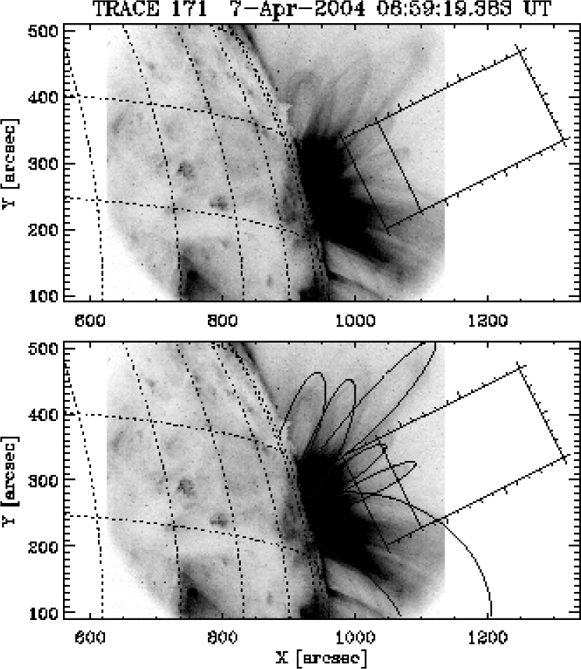
Figure 4: top: TRACE Fe IX 171 Å image of AR 10582 about 3 hr after the SOLARC magnetic field measurements were taken. The rectangle marks the FOV of the SOLARC observations. The horizontal line within the SOLARC FOV indicates the location where a reversal in the direction of the longitudinal coronal magnetic field as a function of height above the solar limb was observed. bottom: Same as the top panel, with a subset of the magnetic field lines shown in Figure 3 plotted over the TRACE image.

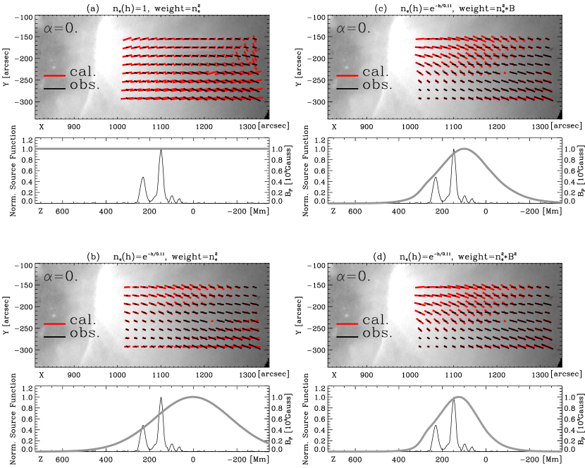
Figure 5: Comparison between observed and synthesized linear polarization maps with four empirical source functions: (a) reference source function with uniform density and temperature distribution, (b) source function based on a gravitationally stratified density distribution and uniform temperature, (c) gravitationally stratified density source function in (b) weighted by the local magnetic field strength, and (d) gravitationally stratified density source function weighted by the local magnetic field energy density, $B^{2}$. The observed (black lines) and synthesized (red lines) linear polarization maps are shown in the top figure in each panel, and the source functions (thick grey lines) from the center of the observed field along the LOS are shown in the bottom figure in each panel. The thin black lines in the bottom figures show the strength of the observed photospheric magnetic flux. The source function in (a) has an equal contribution from every point in space. It is not a physically realistic model and is shown to demonstrate how a simple gravitationally stratified density distribution can affect the outcome of the simulation.

Our 2004 observations were obtained above active region AR 10582 right before its west limb transit. We have obtained the first measurement of the height dependence of the strength of the line-of-sight (LOS) component of the coronal magnetic field in this data, and it showed an intriguing reversal in the direction of the LOS magnetic field at a height of approximately $0.15\ R_{\odot}$ above the solar limb, as shown in Figures 4 and 5 of Lin et al. (2004). This feature and the observed linear polarization map have presented us with our first opportunity to carry out a comprehensive observational test of our coronal magnetic modeling methods in which the strength and direction of the magnetic fields predicted by the models can be directly checked by the observations.

Force-free extrapolation of photospheric magnetic fields is currently the primary tool for the modeling of coronal magnetic fields. However, it is not without limitations or uncertainties. For example, the force-free assumption does not hold true in the photosphere and low chromosphere, and possibly in the high corona above 2 $R_{\odot}$ (Gary, 2001). Moreover, a different assumption (current-free, linear and nonlinear force free) about the state of the electric current in the corona can lead to substantially different extrapolation results. Without direct magnetic field measurements, many fundamental questions concerning the basic assumptions and the validity of our tools cannot be addressed directly. To date, questions like “Is a potential field approximation generally an acceptable approximation for coronal magnetic fields?” or “Do linear or nonlinear force-free extrapolations provide a more accurate description of the coronal magnetic field?” can only be addressed by visual comparison between the morphology of selected field lines of the extrapolated magnetic field model and observational tracers of coronal magnetic fields such as the loops seen in EUV images. However, these visual tests are qualitative and subjective. Furthermore, they assume the coalignment between the magnetic field lines and the loops in EUV images, which has not been verified observationally.

As our first test, we attempted to address the question “Is the potential field extrapolation generally an acceptable approximation for the coronal magnetic field?” This test was conducted by comparing the observed polarization maps of AR 10582 to those derived from a coronal magnetic field model constructed from the potential field extrapolation of photospheric magnetic field data. However, before we present our study, we should point out that because of the nature of our modeling tools and observational data, the results and conclusions of this research are subject to certain limitations and uncertainties. One of the intrinsic limitations of the observational data used in this study is that because of our single sight line from Earth to the Sun, the photospheric and coronal magnetic field observations cannot be obtained simultaneously. In the case of global coronal magnetic field models, the whole-Sun photospheric magnetic field data used as the boundary condition of the extrapolation can be obtained only over an extended period of time. Although the large-scale magnetic structure of nonflaring active regions may appear stable over a long period of time, high-resolution EUV observations have shown that the small-scale coronal structures are constantly changing. Thus, studies such as ours that compare coronal magnetic field observations and models constructed from photospheric magnetic fields inevitably are subject to uncertainties due to the evolution of the small-scale structures in the regions, and we should not expect a precise match between the observed and synthesized polarization maps.

Another deficiency due to the single sight line of our observations is the lack of knowledge of the source regions of the coronal radiation. This is perhaps the most limiting deficiency of the observations and models of this research. The uncertainty of the location of the source regions associated with coronal intensity observations due to the low optical density of the coronal plasma and the resulting long integration path length is familiar. In the case of the coronal magnetic observations, the LOS integration problem prevents us from performing an inversion of the polarization data to reconstruct the three-dimensional magnetic field structure of the corona for direct comparison with those derived from extrapolations or MHD simulations. On the other hand, since extrapolation techniques do not include the thermodynamic properties of the plasma in the construction of the coronal magnetic field models, they do not include information about the location of the CEL source regions either. Therefore, they cannot predict the intensity and polarization distribution of the CEL projected on the plane of the sky that are needed for direct comparison with the polarimetric observations.

Without the information about the location of the source regions from the observational data and the extrapolated models, we adopted a trial-and-error approach in which synthesized linear and circular polarization maps were derived using empirical source functions and the extrapolated potential magnetic field model, and were compared directly with those obtained from observations. Obviously, if acceptable agreement can be achieved with any of the models tested, then we can argue with a certain degree of confidence that these models are plausible models of the observed corona and that the potential field approximation is a reasonable approximation of the coronal magnetic fields. Nevertheless, we should emphasize that this trial-and-error approach is not an exhaustive search of all the possible source functions and therefore cannot provide a clear-cut true-or-false answer. In other words, even if no acceptable agreement can be found with all the model source functions we have considered, the potential field approximation still cannot be dismissed completely.

2 Data Analysis and Results

2.1 Modeling the Coronal Magnetic Fields

2.1.1 Evolutionary History of AR 10581 and AR 10582

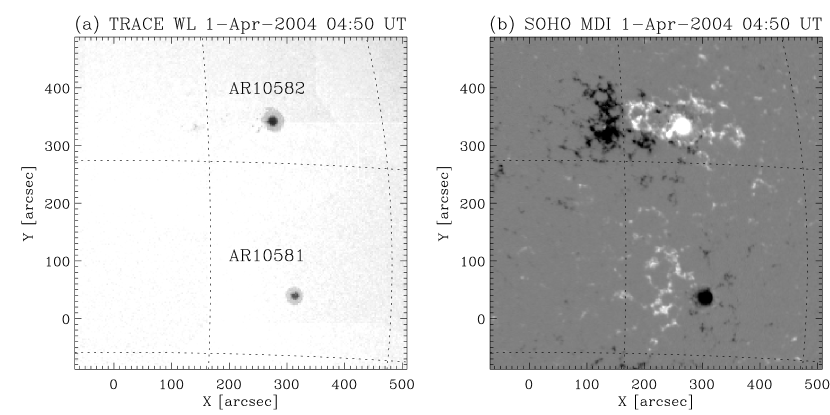
Figure 1: TRACE white-light image (left) and SOHO/MDI magnetogram (right) of AR 10581 and AR 10582 observed on the solar disk show the regions’ photospheric intensity and magnetic field configuration.

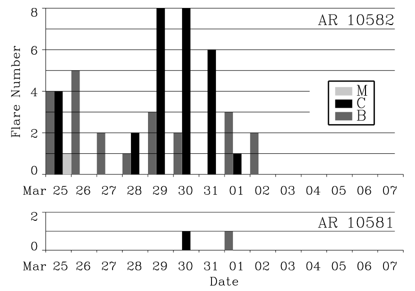
Figure 2: Flare counts of AR 10581 and AR 10582 from 2004 March 25 to 2004 April 07.

Although the purpose of this study is to test the validity of potential field approximation for AR 10582, examination of the photospheric magnetic field configuration and evolution of the regions should be informative and helpful for assessing the results of this study. Figure 1 shows the TRACE (Transition Region and Coronal Explorer) white-light image and the SOHO/MDI (Solar and Heliospheric Observatory/Michelson Doppler Imager) magnetogram of these regions on 2004 April 1. Their activity history during their disk transit is shown in Figure 2. AR 10581 and 10582 first appeared on the east limb of the Sun on 2004 March 23. Images taken by SOHO/EIT (Extreme-ultraviolet Imaging Telescope) and TRACE data showed that AR 10582 was initially very active and produced several C- and M-class flares between March 23 and April 1. AR 10581, on the other hand, produced only two small flares in the first week. No flare activities were observed from either region in the four days before the SOLARC observation. Close examination of EIT and TRACE data also showed that the large-scale configuration of these active regions did not change significantly during this period.

2.1.2 Extrapolated Potential Field Model of AR 10582

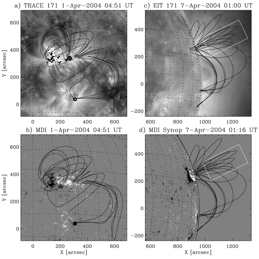
Figure 3: Selected extrapolated magnetic field lines plotted over Fe IX 171 Å images and SOHO/MDI magnetograms of AR 10581 and AR 10582 when these regions are observed on the solar disk (a and b) and at the west limb (c and d).

We employed a global potential field extrapolation program based on the Green’s Function method developed by Schatten et al. (1969) and Sakurai (1982) for the construction of the coronal magnetic field (Liu & Zhang, 2002). The magnetic synoptic map of Carrington Rotation 2014 obtained by the SOHO/MDI instrument was used as the boundary condition of the extrapolation. The first two panels, (a) and (b), of Figure 3 show selected field lines from the extrapolated coronal magnetic field model of AR 10581 and AR 10582 plotted over a TRACE Fe IX 171 Å image as they are viewed on the disk. Panels (c) and (d) show the same set of field lines overplotted on the SOHO/EIT Fe IX 171 Å images and SOHO/MDI magnetograms when they transited the west limb. The field of view of the SOLARC LOS magnetogram observation is marked by the rectangular box in the figure. We found a general agreement between the orientation and distribution of the discernible EIT intensity loops during the time of the SOLARC observations, and the selected magnetic field lines from the extrapolated model are evident. The extrapolated magnetic field lines in AR 10582 are predominantly aligned along the east-west direction, while a set of field lines running along the north-south direction connecting the two active regions also coincide with a large north-south loop in the EIT images. Figure 4 shows a TRACE high-resolution Fe IX 171 Å image of AR 10582 taken about 3 hr after the limb spectropolarimetric observations had ended. We found that a subset of the extrapolated field lines appear to closely resemble the TRACE loops. While the similarities in the morphology of the EUV intensity images and the extrapolated magnetic field lines seem to suggest that the extrapolated coronal magnetic field model is a fair representation of the magnetic field configuration of AR 10581 and AR 10582, it is a subjective interpretation.

2.2 Observational Test of the Potential-Field Coronal Magnetic Field Model

2.2.1 Synthesis of the Coronal Polarization Maps

We have developed a program to calculate the LOS integrated linear and circular polarization signals at any point in the plane of the sky (POS) given the extrapolated coronal magnetic field model and the density and temperature distribution of the solar corona based on the classical theory of Lin & Casini (2000) for the forbidden CEL polarization. The formulae for the emergent Stokes parameter of the CEL are identical to those derived from a full-quantum mechanical formulation (Casini & Judge, 1999), up to a proportional constant. However, as this classical formulation does not consider the effect of collisional depolarization, it may overestimate the degree of linear polarization at a lower height. The azimuth angle of the linear polarization predicted by our program should also be affected slightly when we integrate over a long path length, since the collisional depolarization effect may change the relative contribution of the sources along the LOS. Judge & Casini (2001) have also developed a CEL polarization synthesis program that includes the effect of collisions. We have implemented both programs to generate the linear and circular polarization signals from the extrapolated potential field model. We found that the synthesized polarization maps derived from these two programs are very similar, and analysis based on these two programs yielded the same results. The comparison of the synthesized polarization maps from these two programs will be presented when we present the study comparing the observed and synthesized polarization maps.

2.2.2 Linear Polarization Maps

The 2004 April 6 data include a linear polarization scan encompassing both AR 10581 and AR 10582. However, due to the long integration time required, only one circular polarization measurement was obtained above AR 10582. Therefore, this study concentrates on the $320\arcsec\times 160\arcsec$ field with both circular and linear polarization measurements as marked by the rectangular area in Figures 3 and 4. As it was mentioned in §1, the lack of knowledge of the coronal density and temperature distribution is the greatest uncertainty in our study. Nevertheless, based on decades of observations, we now know that strong coronal emissions are always associated with active regions. Furthermore, due to the small density scale height of the high-temperature emission lines, the contribution function of the CELs along the LOS is heavily weighted toward layers close to the POS containing Sun center. Therefore, we can expect that for isolated active regions, the forbidden coronal emission originates from a localized region near the POS containing Sun center during the active region’s limb transit. According to the SOHO/MDI white-light archive, there were no other active regions present on the solar disk on 2004 April 1, when AR 10581 and AR 10582 were located approximately at disk center. Additionally, there was no evidence of new active regions emerging in the vicinity of these regions up to the day of the coronal polarization measurement. Therefore, it is reasonable to assume that the polarized radiations we measured originated in the corona above these active regions near the POS containing Sun center. This expectation prompted us to test if an empirical source function constructed from a simple gravitationally stratified atmosphere and local magnetic field properties, such as the strength or the magnetic energy, can reproduce (if only qualitatively) the observed polarization maps.

For our first test, we constructed a linear polarization map using a source function ${W_{n_{e}}}(\bf{r})$ that is proportional to the square of the density of a spherically symmetric, gravitationally stratified density distribution with a density scale height of $h_{0}=83$ Mm ($0.11\ R_{\odot}$, Lang, 1984). That is,

$$W_{n_{e}}({\bf r})=e^{-2h({\bf r})/h_{0}},$$ (1)

where ${\bf r}$ is the three-dimensional position vector in the heliocentric coordinate system and $h({\bf r})$ is the height at ${\bf r}$. The temperature of the corona was assumed to be constant and did not affect the source function. The magnetic properties of the corona are not included in this model either. This is similar to the atmospheric model used in the polarization synthesis performed by Judge et al. (2006). The resulting normalized source function along the LOS in the center of the SOLARC field of view and the synthesized linear polarization map are shown in panel (b) of Figure 5. Note that because AR 10582 was located between W70 to W80 longitude, this density-only source function has its maximum located outside of the active region. Although $W_{n_{e}}({\bf r})$ is obviously a gross simplification of the magnetic coronal atmosphere, and we should not expect to see good agreement between the observed and synthesized linear polarization maps based on $W_{n_{e}}({\bf r})$ alone (as demonstrated in the top figure in panel (b) of Figure 5), this test is a necessary step in our systematic trial-and-error study. Furthermore, the importance of its inclusion in the estimate of the source function can be seen when we compare the linear polarization maps constructed with and without it (top figure in panel (a) of Figure 5).

In our next test, we examined if there is any simple relationship between the CEL source function and the magnetic properties of the corona. Because of the observed correlation between the strong CEL radiation and active regions, it is only logical to test if a source function with its amplitude proportional to the local magnetic field strength or magnetic energy can reproduce the observed polarization signals. To test this idea, we multiplied the source function that was constructed from the uniform temperature, gravitationally stratified atmosphere model by the local magnetic field strength $B$. Another model used the local magnetic field energy density $B^{2}$ as the additional magnetic weighting function. Accordingly, the two magnetic source functions are expressed by

$$W_{B}({\bf r})=e^{-2h({\bf r})/h_{0}}B$$ (2)

and

$$W_{B^{2}}({\bf r})=e^{-2h({\bf r})/h_{0}}B^{2}.$$ (3)

The additional magnetic constraints restrict the source function to a more localized region around the active region, and with a spatial scale comparable to that of the active region. However, the linear polarization maps derived using these source functions still are not in good agreement with the observed one. These are demonstrated in panels (c) and (d) of Figure 5.

Although none of the linear polarization maps we have constructed so far can be considered to be in good agreement with the observation, it can be argued that the maps derived from the two source functions with magnetic constraints appear to better match the observed one, especially at the lower right-hand corner of the field, where the degree of linear polarization is the highest. Therefore, we suspect that the assumption about the magnetic dependence of the CEL source function is in general valid. However, the correlation may be occurring at a spatial scale smaller than that of the active regions. Because space EUV observations have shown that radiation from the emission-line corona originates from loop-like structures with a characteristic size much smaller than the characteristic size of the active regions, it should not be surprising that the linear polarization maps produced by the broad source functions do not agree well with the observation. This reasoning prompted us to experiment with source functions with a spatial scale approximately equal to a few times the characteristic width of the coronal loops to test if better agreement between the observed and synthesized polarization maps can be achieved.

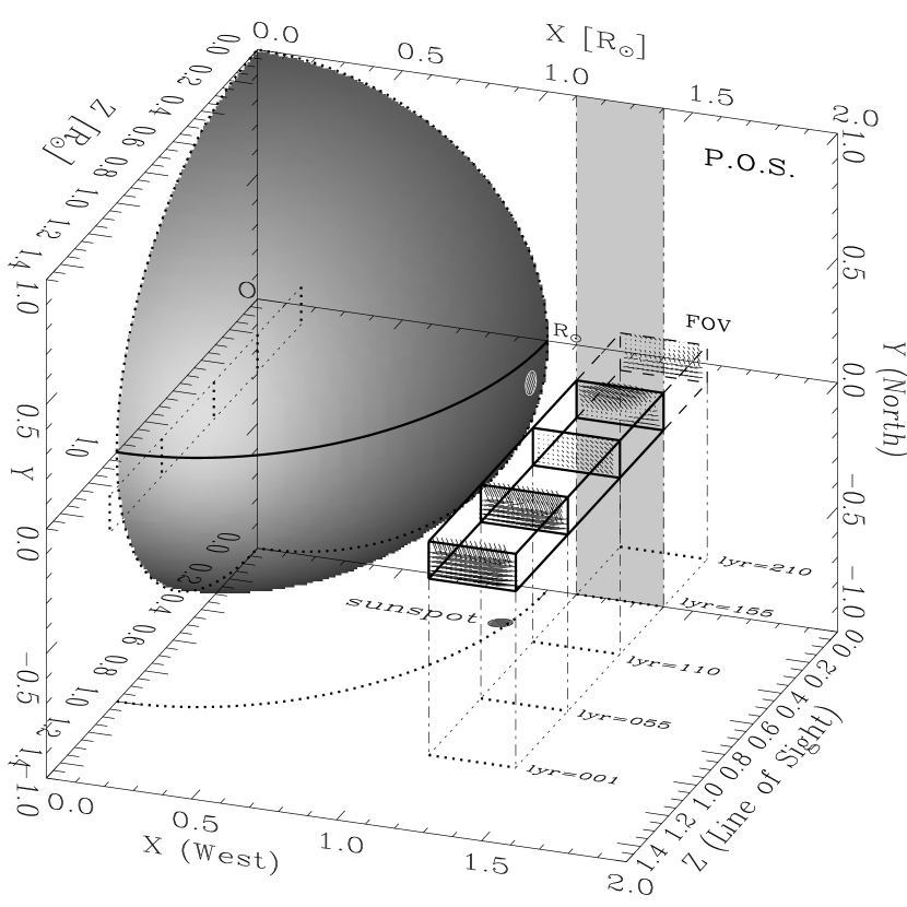
Figure 6: Three-dimensional plot to illustrate the locations of the thin layers along the LOS, and their relationship to the solar sphere and the sunspot of AR 10582. The Sun is represented by the shaded quarter sphere. The observing LOS is along the $Z$ axis. Layer 155 is located in the POS containing the Sun center.

Since we do not have information about the location of the source regions of the observed Fe XIII 10747 Å line emission at this spatial resolution, we constructed the linear polarization map of 205 layers along the LOS within the SOLARC FOV for comparison with the observed linear polarization map. The separation between the synthesized layers is 4.5 Mm, the resolution of the potential field extrapolation calculation. The first and last layers are located 720 Mm (or about 1000$\arcsec$) in front and 250 Mm (or about 340$\arcsec$) behind the POS containing Sun center, respectively. The locations of these layers with respect to the solar sphere, the observed active region, and the LOS of the observer are illustrated in Figure 6. We used a one-dimensional Gaussian function with a full width at half-maximum (FWHM) in the LOS direction equal to a few times that of the characteristic coronal loop size to model the source function. For this test, we adopted the 8 Mm characteristic loop width of the EUV Fe XIV 28.4 nm line derived by Aschwanden et al. (2000). This line is chosen because its ionization temperature of $2.2\times 10^{6}$ K is closer to that of the IR Fe XIII 10747 Å line ($T_{\rm ion}=1.7\times 10^{6}$ K) than the other SOHO/EIT EUV lines. We calculated and compared the polarization maps with the FWHM of the source function set from 1 to 14 times the characteristic loop width of the Fe XIV 28.4 nm lines and found no significant difference between the polarization maps. This is expected, since the coronal magnetic field should vary slowly in space as it expands to fill the entire coronal volume. Finally, because of this lack of sensitivity in the synthesized polarization signals to the variations of the FWHM of the source function, we used a nominal 56 km FWHM source function (or 7 times the FWHM of the Fe XIII 28.4 nm loops) for the calculation of the synthesized polarization maps in the rest of the paper.

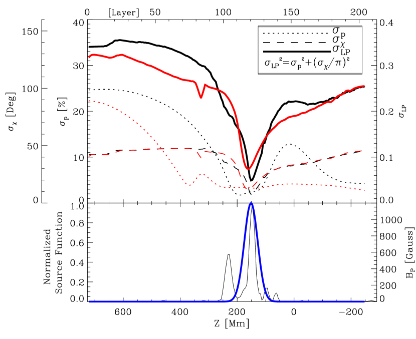
Figure 7: top: The rms errors between the synthesized and observed linear polarization amplitude, $\sigma_{p}$ (dotted lines), azimuthal angle, $\sigma_{\chi}$ (dashed lines), and the combination of the two, $\sigma_{LP}$ (thick solid lines). Results derived with the coronal polarization synthesis program developed by the authors and Judge & Casini (2001) are shown in black and red, respectively. Best-fit position for linear polarization occurs at approximately layer 120, right above the sunspot. bottom: The thin solid line shows the magnitude of the LOS magnetic field of the photosphere. The thick blue line shows the source function along the LOS for layer 120.

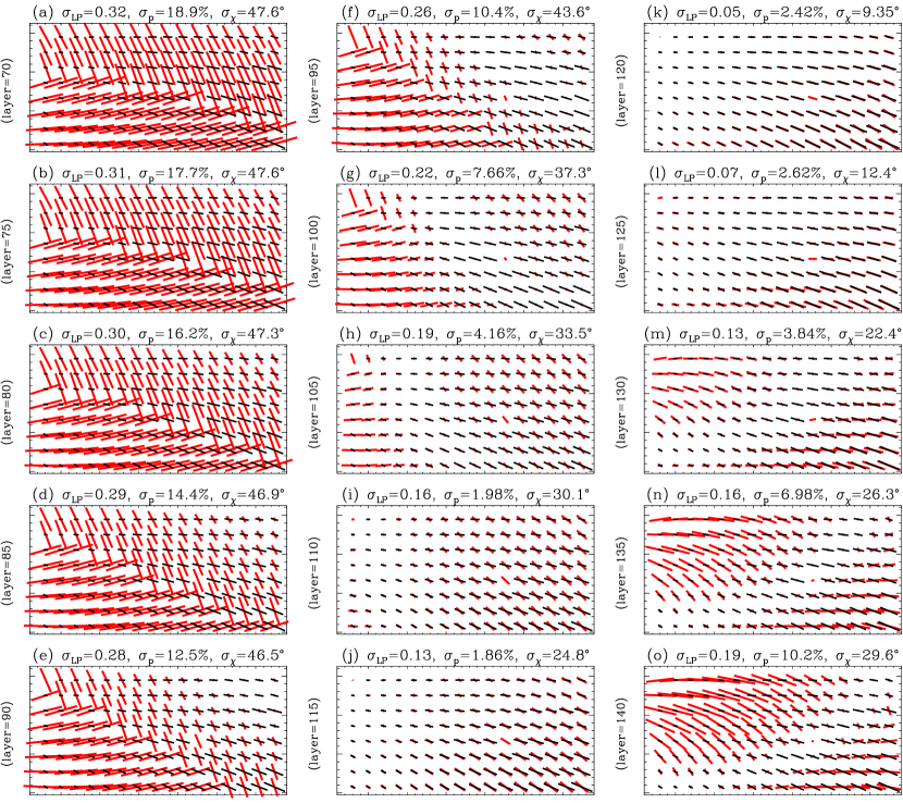
Figure 8: The observed (black lines) and synthesized (red lines) linear polarization maps derived with our classical synthesis program from 15 layers along the LOS near the active region. Layer 120 is the layer with the smallest rms error.

We evaluated the quality of the fit between the synthesized and observed polarization maps from the rms difference between the degree of polarization $p$ and the azimuthal angles $\chi$ of the linear polarization direction projected in the POS, $\sigma_{p}$ and $\sigma_{\chi}$, respectively. Figure 7 shows $\sigma_{p}$ and $\sigma_{\chi}$ as functions of $z$ along the LOS. Results derived from our own collisionless classical formulation are shown by the black lines, and those derived with Judge & Casini’s code (2001; hereafter referred to as the JC synthesis code) are shown in red. Figure 7 shows that the minimum of $\sigma_{p}$ and $\sigma_{\chi}$ both occur near the layer right above the sunspot of the active region. Figure 8 shows 15 synthesized linear polarization maps calculated with our classical synthesis code from layer 70 to layer 140, with an interval of 5 layers, plotted over the observed map. The best fit, determined from the total rms error $\sigma^{2}_{lp}=\sigma^{2}_{p}+(\sigma_{\chi}/\pi)^{2}$ of the linear polarization maps, occurs around layer 120, right above the sunspot.

2.2.3 Comparison with Judge & Casini’s Coronal Polarization Synthesis Code

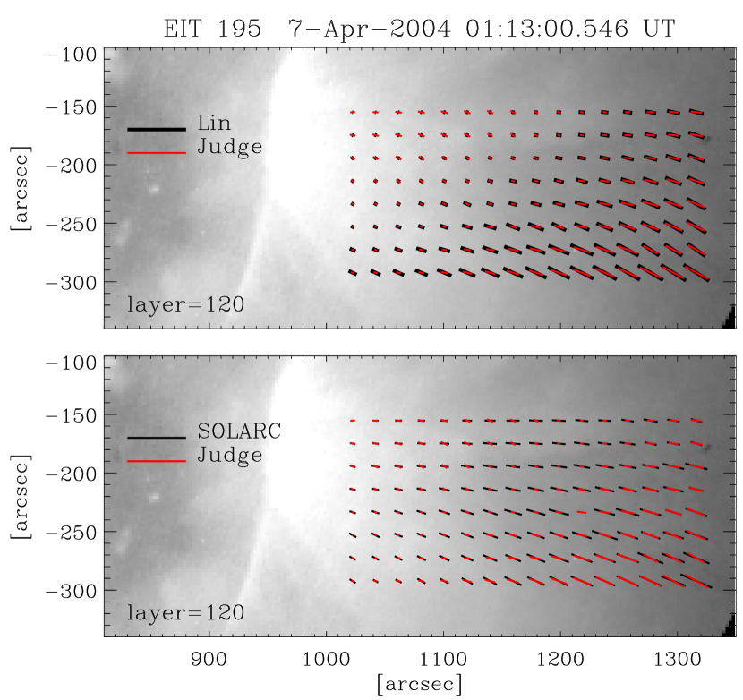
Figure 9: top: The linear polarization maps derived from Judge & Casini’s synthesis program (red lines), and from Liu and Lin’s classical synthesis program (black lines). bottom: Comparison of the linear polarization map derived from Judge & Casini’s program and that observed by SOLARC.

Figure 9 shows the linear polarization map of layer 120 derived with the JC synthesis code compared with that derived from our collisionless code, and with observations. Apparently, the JC synthesis code consistently predicts a smaller linear polarization amplitude compared with our classical theory, as expected, and produced better agreement with the observed linear polarization map at the lower part of the field. However, there are still significant disagreements in the upper part of the field, where both the JC synthesis code and our own program overestimated the degree of linear polarization. This may be due to the larger measurement errors associated with the small amplitudes of the observed linear polarization, and their significance should not be overstated. Close examination of the data shows that the larger rms error shown in Figure 7 in the JC results is due to larger errors in this region. Therefore, we do not consider that our collisionless synthesis actually provides better agreement with the observations.

In view of the inherent uncertainties in the modeling process discussed in §1, we do not feel that a meaningful quantitative comparison between these two methods can be justified at this point. Nevertheless, Judge & Casini’s program with collisional depolarization is definitely a more complete description of the physical processes in the atmosphere of the solar corona and should be preferred. Future observations at a lower height, where the collisional depolarization effect is expected to be more important, should allow us to clearly distinguish between the effect of collisional depolarization and uncertainties in the modeling process.

2.2.4 Strength and Reversal of Line-of-Sight Magnetic Fields

Our analysis so far has demonstrated that the potential field model can reproduce the observed linear polarization maps. Is this a coincidence? To answer this question, it is interesting to first note that the layers of best fit for both the degree and azimuthal angle of the linear polarization occur at approximately the same location near the region of the strongest photospheric magnetic fields. Since $\sigma_{p}$ and $\sigma_{\chi}$ were determined independently, the probability that these two parameters reach minimum at approximately the same location and at the region with the strongest photospheric magnetic flux purely by chance should be very low. Therefore, we believe that our analysis of the linear polarization maps support the idea that the potential field model is a good approximation of the real coronal magnetic field of AR 10582. Furthermore, if an agreement between the modeled and observed height dependence of the LOS component of the coronal magnetic field can be found, then the validity of the potential field model, at least as a first order approximation for stable active regions, can be strongly argued.

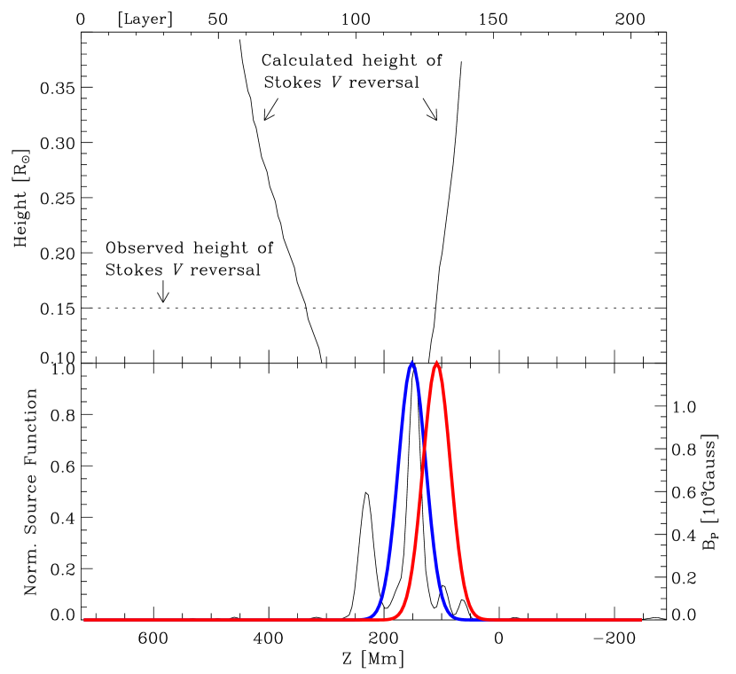
Figure 10: top: The calculated height of Stokes $V$ reversal as a function of height from the limb derived from the potential field model. bottom: Similar to Figure 7, the thin solid line shows the magnitude of the LOS magnetic field of the photosphere, and the thick blue line shows the source function of layer 120 where the best fit for the linear polarization map occurs. The thick red line shows the source function along the LOS for layer 130.

To check if the observed Stokes $V$ reversal can be reproduced, we derived the height of Stokes $V$ reversal $H_{0}$ for each of the 205 56-Mm-FWHM layers along the sight line. The LOS components of the magnetic field $B_{z}$ in the central $320\arcsec\times 80\arcsec$ region of each layer were averaged in the north-south direction (or the tangential direction with respect to the local solar limb) to simulate the spatial averaging performed on the observation data. The result is shown in Figure 10. Since the dominant magnetic structure around the active region in our FOV consists of magnetic loops oriented along the east-west direction, there were two locations with $H_{0}=0.15\ R_{\odot}$, one due to the front (closer to the observer) portion of the loops near layer 80, and one located in the back of the loops, at layer 130. Note that layer 130 is much closer to the sunspot of AR 10582 and the maximum of the empirical source functions $W_{B}$ and $W_{B^{2}}$ shown in Figure 5. In comparison, the amplitudes of $W_{n_{e}}$, $W_{B}$, and $W_{B^{2}}$ at layer 80 are only about 0.15, 0.1, and 0.05, respectively (Figure 5). We calculated the net Stokes $V$ signals as a function of height above the limb for layer 130 and found that they agree well with the observed signals as shown in Figure 11. On the other hand, this is not the case for layer 80. We conducted the same analysis using the JC synthesis code and produced virtually identical results. Therefore, it is more likely that the dominant source of the Stokes $V$ signals originates from around layer 130.

The blue and red Gaussian curves in Figure 10 mark the locations where the best fits to the linear and circular polarization observation occur, respectively. As is clearly shown in this figure, layer 130 is only about 50 Mm away from the location with the best fit of the linear polarization maps. Given the proximity of the locations of the best fit of the three parameters ($p$, $\chi$, and $H_{0}$) and the strongest magnetic feature of the active region, we concluded that this comparative study demonstrates the validity of potential field extrapolation as a tool for the modeling of the coronal magnetic field.

3 Summary, Discussions, and Conclusions

This research examines observationally the validity of current-free, force-free potential-field approximation for coronal magnetic fields. We conducted a study comparing observed and synthesized spatial variations of the linear and circular polarization maps in the corona above active region AR 10582, which after a week of extensive flaring activities should have settled into a minimum energy configuration that could be adequately modeled by a potential field model. The coronal magnetic field model used for this study was constructed from a global potential field extrapolation of the synoptic photospheric magnetogram of Carrington cycle 2014 obtained by the SOHO/MDI instrument. Because the most important source of error of this type of study is the uncertainty of the location of the source function of the coronal radiation, we first tested three analytical, but empirically determined, source functions. These simple source functions are based on a gravitationally stratified atmospheric density model with a uniform temperature in the entire modeled volume, supplemented by magnetic weighting functions based on the observational impression that, at least at the length scale of the typical active region size, CEL radiation seems to be correlated with the strength of the photospheric magnetic fields. We found that none of these empirical source functions can adequately reproduce the observed linear polarization maps, although it seems that the source functions that include both density and magnetic fields produced slightly better results. Based again on the observational impression that the coronal intensity structures have a spatial scale much smaller than that of the active regions, we then compared the observed polarization maps with those constructed from thin (56 Mm FWHM) layers along the LOS. In this analysis, we found that polarization maps originating from layers located near the sunspot of the region are in reasonable agreement with the observed ones. However, the best fit for linear and circular polarization did not occur at the same layer. They are separated by a distance of about 50 Mm.

Does the small discrepancy between the best-fit locations of the linear and circular polarization weaken the support for the potential field extrapolation? As we have discussed in §1, many uncertainties conspire to limit the precision of this study. For example, the difference may be due to the evolution of the small-scale photospheric magnetic field of the active region, and we do not have any observational information that we can use to test this possibility. The assumption of uniform temperature distribution in our source function is certainly not a physically realistic assumption. Therefore, it is not possible to assess the significance of the small difference in the location of the source regions of the linear and circular polarization. Furthermore, in addition to density and temperature, the source functions of CEL linear and circular polarization depend on different components of the coronal magnetic field. So it is in fact physically reasonable that we would find the linear and circular polarization signals originate from slightly different locations. Finally, because the three parameters ($\sigma_{p}$, $\sigma_{\chi}$, and $H_{0}$) we used to evaluate the quality of the fit were obtained independently, the statistical significance that all three parameters reached minimum at approximately the same location near the strongest photospheric magnetic feature of the active region cannot be dismissed as pure coincidence. These considerations lead us to conclude that potential field extrapolation can be used to provide a zero-order approximation of the real solar corona if the active region is in a relatively simple and stable configuration. Additionally, this study suggests that, at least for isolated active regions, CEL radiation may originate from a region close to the strongest photospheric magnetic feature in the active region with a small spatial scale comparable to the characteristic size of the coronal loops seen in the intensity images. If this is confirmed, then a single-source inversion to infer the magnetic field directly from the polarimetric observation such as that proposed by Judge (2007) may be justified.

Our conclusion about the viability of potential field extrapolation as a coronal magnetic field modeling tool for stable active regions is supported by a study by Riley et al. (2006), in which the coronal magnetic field configuration derived from a potential field model was found to closely match that derived from a MHD simulation in the case of untwisted fields. Nevertheless, we should emphasize that our conclusion is derived from a single observation of a simple and stable active region. Clearly, more observations and model comparison are needed for a more comprehensive test of this result.

Can the potential field approximation be used to model more complicated active regions? Using radio observations, Lee et al. (1999) found that a force-free-field model yields better agreement between the temperatures of two isogauss surfaces connected by the modeled field lines of an active region with strong magnetic shear. This study thus provides observational evidence against the use of potential field approximations for the modeling of complex active regions. Therefore, linear and nonlinear force-free extrapolations should be employed in future testing of theoretical coronal magnetic field models using the IR spectropolarimetric observations to study if these models can offer a better description of the observed coronal fields.

Can we distinguish the potential coronal magnetic field configurations from the non-potential ones with the spectropolarimetric observations of the coronal emission lines? In a numerical study, Judge (2007) has demonstrated the sensitivity of LOS-integrated coronal polarization measurements to the electric current in the corona using theoretical coronal magnetic field models as input. Therefore, we should expect to find better agreement between observed and synthesized polarization maps for more complex active regions with linear or nonlinear force-free magnetic field models. Work to model AR10582 using the force-free extrapolation method is already underway, and we should be able to address this question in the near future. Since all extrapolation methods are subject to the ambiguities problem of the source regions, we will also employ MHD simulations that include both the magnetic and thermodynamic properties of the corona in the calculation to help resolve this problem. These are research activities that we will be pursuing in the near future as the solar cycle evolves toward the next solar maximum and more coronal magnetic field data become available.

The greatest difficulty of this study is the uncertainty of the location of the source function due to the long integration path along the LOS. However, this is not a difficulty affecting only the interpretation of coronal magnetic field measurements. It affects the intensity observation as well, and is the primary reason that years into the operation of SOHO/EIT and TRACE, we still cannot deduce 3-D intensity and temperature structure of the corona using data from these instruments. Fortunately, this deficiency in our observing capability may finally be removed with the recent launch of the STEREO mission (Solar TErrestrial RElations Observatory). For the resolution of the LOS integration problem in polarimetric observations, Kramar et al. (2006) have demonstrated the promising potential of vector tomography techniques. While stereoscopic coronal magnetic field observations will not be realized any time soon, this method can be applied to observations obtained over periods of several days during the limb transit of active regions, provided that the active regions are in a stable condition. This is perhaps the best observational tool available for the resolution of the LOS integration problem in the near future.

Figure 11: The observed (solid line with star and error bars) and synthesized net circular polarization signals from the source layer 130 (dotted line) and layer 80 (dashed line) are plotted as a function of distance from the solar limb.

References

- Arnaud, J. (1982) Arnaud, J. 1982, A&A, 112, 350
- Aschwanden et al. (2000) Aschwanden, M. J., Alexander, D., Hurlburt, N., Newmark, J. S., Neupert, W. M., Klimchuk, J. A., & Garry, G. A. 2000, ApJ, 531, 1129
- Brosius & White (2006) Brosius, J. W., & White, S. M. 2006, ApJ, 641, L69
- Casini & Judge (1999) Casini, R., & Judge, P. G. 1999, ApJ, 522, 524
- Eddy & Malville (1967) Eddy, J.A., & Malville, M. J. 1967, ApJ, 150, 289
- Gary (2001) Gary, G. A. 2001, Sol. Phys., 203, 71
- Judge (2007) Judge, P. 2007, ApJ, 662, 677
- Judge & Casini (2001) Judge, P. G., & Casini, R. 2001, in ASP Conf. Ser. 236, Advanced Solar Polarimetry: Theory, Observation, and Instrumentation, ed. M. Sigwarth (San Francisco: ASP), 503 (JC)
- Judge et al. (2006) Judge, P., Low, B. C., & Casini, R. 2006, ApJ, 651, 1229
- Kramar et al. (2006) Kramar, M. B., Inhester, B., & Solanki, S. K. 2006, A&A, 456, 665
- Lang (1984) Lang, K. 1980, Astrophysical Formulae (Berlin: Springer)
- Lee et al. (1999) Lee, J., White, S. M., Kundu, M. R., McClymont, A. N., & Mikić, Z. 1999, ApJ, 510, 413
- Lin & Casini (2000) Lin, H., & Casini, R. 2000, ApJ, 542, 528
- Lin et al. (2004) Lin, H., Kuhn, J. R., & Coulter, R. 2004, ApJ, 613, L177
- Lin et al. (2000) Lin, H., Penn, M. J., & Tomczyk, S. 2000, ApJ, 541, L83
- Liu & Zhang (2002) Liu, Y., & Zhang, H. 2002, Publ. Yunnan Obs., 92, 1
- Mickey (1973) Mickey, D. L. 1973, ApJ, 171, L19
- Querfeld (1982) Querfeld, C.W. 1982, ApJ, 255, 764
- Riley et al. (2006) Riley, P., Linker, J. A., Mikić, Z., & Lionello, R. 2006, ApJ, 653, 1510
- Sakurai (1982) Sakurai, T. 1982, Sol. Phys., 76, 301
- Schatten et al. (1969) Schatten, K. H., Wilcox, J. M., & Ness, N. F. 1969, Sol. Phys., 6, 442
- Tomczyk et al. (2007) Tomczyk, S., McIntosh, S. W., Keil, S. L., Judge, P. G., Schad, T., Seeley, D. H., & Edmondson, J. 2007, Science, 317, 1192