Computational Model for Electron-Nucleon Scattering and Weak Charge of the Nucleon

Abstract

We show how computational symbolic packages such as FeynArts, FormCalc, Form and LoopTools can be adopted for the evaluation of one-loop hadronic electroweak radiative corrections for electron-nucleon scattering and applied to calculations of the nucleon weak charge. Several numerical results are listed, and found to be in good agreement with the current experimental data.

I Introduction

Next-to-Leading-Order (NLO) effects in electroweak interactions play a crucial role in tests of the Standard Model, and require careful theoretical evaluation. An excellent place to search for new physics, the deviation of the weak charge of the nucleon from its Standard Model prediction also requires considerable experimental and theoretical input. The importance of theoretical predictions for the weak charge of the nucleon was recognized more that two decades ago by Marciano and Sirlin (MS84, ). Their original analysis was followed recently by significant theoretical work on the proton weak charge (EKM2003, ), which presented an updated Standard Model prediction for the weak charge of the proton, and estimated the QCD structure uncertainties.

Computer packages such as FeynArts (FeynArts, ), FormCalc (FormCalc, ), LoopTools (LoopTools, ), (FF, ) and Form (Form, ) have created the possibility to go one step further. Now, we have an option of calculating parity-violating NLO effects including all of the possible loop contributions within a given model. We have already tested the automated approach to calculate one-quark radiative corrections (BAB2002, ).

In the work presented here, we adopt FeynArts and FormCalc for the NLO symbolic calculations of amplitude or differential cross section in electron-nucleon scattering. Using Dirac and Pauli-type couplings with the monopole form factor approximation, we construct the computational model enabling FeynArts and FormCalc to deal with electron-nucleon scattering up to the NLO level. Since the weak charge of the nucleon is directly related to the form factors of the parity-violating part of the amplitude at the zero momentum transfer, we choose the calculation of the weak charge of the nucleon to be a suitable test our method. Within the uncertainty, which mostly comes from the uncertainty of the current electromagnetic form factor measurements, our results agree with experiment.

We start with expressions for Pauli and Dirac couplings in terms of fermion weak and electric charges, and the definition and classification of one-loop radiative corrections. After that, an example for the $\left\{\gamma-Z\right\}$ box type of correction for electron-proton scattering is considered and a computational model is proposed. We proceed with computational details for the self-energy graphs and vertex correction graphs. Since we reserve full kinematic dependence in all types of our NLO calculations, it will make it easier to adopt our results to the current and future parity-violating experiments.

II Theory

II.1 Dirac and Pauli Coupling

In the approximation where the nucleon behaves as a point-like particle, vector boson couplings obey general rules of electroweak theory. For left and right handed fermions, we can use the following structure for the $\left\{Z-N\right\}$ type couplings:

$$\Gamma_{\mu}^{Z-N}=ie\,\left[g_{L}^{Z-N}\gamma_{\mu}\varpi_{-}+g_{R}^{Z-N}\gamma_{\mu}\varpi_{+}\right],$$ (1)

where $\varpi_{\pm}=\frac{1\pm\gamma_{5}}{2}$ are chirality projectors and $g_{L,R}^{Z-N}$ represents the coupling strength for the left and right handed fermions, respectively. Substitution of $\varpi_{\pm}$ into Eq.(1) yields the vector and axial vector representation of the coupling $\Gamma_{Z-N}^{\mu}$:

$$\Gamma_{\mu}^{Z-N}=ie\,\left[\frac{g_{L}^{Z-N}+g_{R}^{Z-N}}{2}\gamma_{\mu}+\frac{g_{R}^{Z-N}-g_{L}^{Z-N}}{2}\gamma_{\mu}\gamma_{5}\right].$$ (2)

Couplings of vector bosons to fermions derived from the neutral current part of the electroweak Lagrangian predict tree-level values of $g_{L}^{Z-N}$ and $g_{R}^{Z-N}$ given by:

$$\frac{g_{L}^{Z-N}+g_{R}^{Z-N}}{2} = \frac{1}{4}\frac{C_{3}-4s_{w}^{2}Q}{c\,_{w}s_{w}},$$

$$\frac{g_{R}^{Z-N}-g_{L}^{Z-N}}{2} = -\frac{1}{4}\frac{C_{3}}{c_{w}\,s_{w}}.$$

Here, $C_{3}$ and $Q$ are twice the value of the isospin and electric charge respectively, and $s_{w}$ and $c_{w}$ are $\sin\theta_{W}$ and $\cos\theta_{W}$, where $\theta_{W}$is a Weinberg mixing angle. In the case when a photon couples to the nucleon, $g_{L}^{\gamma-N}=g_{R}^{\gamma-N}=Q$ and $\Gamma_{\mu}^{\gamma-N}=ieQ\gamma_{\mu}$.

To accommodate nucleon structure, we have the couplings preserve their vector and vector-axial structure, but with the charges replaced by the corresponding form factors. The electromagnetic $\Gamma_{\mu}^{\gamma-N}$ coupling has two vector components responsible for static electric and magnetic interactions:

$$\Gamma_{\mu}^{\gamma-N}\left(q\right)=ie\left[F_{1}\left(q\right)\gamma_{\mu}+\frac{i}{2m_{N}}\sigma_{\mu\alpha}q^{\alpha}F_{2}\left(q\right)\right],$$ (4)

where $F_{1}\left(q\right)$ and $F_{2}\left(q\right)$ are the Dirac and Pauli form factors, respectively, and $q^{\alpha}$ is the four-momentum transferred to the nucleon. As for $\Gamma_{\mu}^{Z-N}\left(q\right)$, we have:

$$\Gamma_{\mu}^{Z-N}\left(q\right)=ie\left[f_{1}\left(q\right)\gamma_{\mu}+\frac{i}{2m_{N}}\sigma_{\mu\alpha}q^{\alpha}f_{2}\left(q\right)+g_{1}\left(q\right)\gamma_{\mu}\gamma_{5}\right],$$ (5)

with $f_{1}\left(q\right)$, $f_{2}\left(q\right)$ and $g_{1}\left(q\right)$ as weak Dirac, Pauli, and axial-vector form factors. According to the first line of the Eq.(LABEL:e1.3), form factors $f_{1}\left(q\right)$ and $f_{2}\left(q\right)$ are expressed as:

$$f_{1,2}\left(q\right)=\frac{1}{4c_{w}s_{w}}\left(F_{1,2}^{V\left(N\right)}\left(q\right)-4s_{w}^{2}F_{1,2}\left(q\right)\right),$$ (6)

with $F_{1,2}^{V\left(p\right)}=-F_{1,2}^{V\left(n\right)}=F_{1,2}^{p}-F_{1,2}^{n}$. For $g_{1}\left(q\right)$ we have

$$g_{1}\left(q\right)=-\frac{1}{4c_{w}s_{w}}g_{A}\left(q\right),$$ (7)

where $g_{A}^{p}\left(q\right)=-g_{A}^{n}\left(q\right)=g_{A}\left(q\right)$ is an axial form factor. To considerably simplify analytical expressions, in our computational model we use the monopole structure for form factors expressed as

$$\left\{F_{1,2},g_{A}\right\}\left(q\right)=\frac{\Lambda^{2}\left\{F_{1,2},g_{A}\right\}\left(0\right)}{\Lambda^{2}-q^{2}},$$ (8)

which is a reasonable approximation in our case. The value of the parameter $\Lambda^{2}=0.83m_{N}^{2}$ is found after the fit of the electromagnetic form factors by monopole approximation in the low momentum transfer region. Further details on how couplings where implemented in the computational model are given in the appendix.

II.2 Definition of NLO Contribution

In order to define the Next-to-Leading-Order hadronic corrections, we are using the electron-nucleon parity violating Hamiltonian in the form proposed by (MS84, ):

$$H^{PV}=\frac{G_{F}}{\sqrt{2}}\left[C_{1N}\left(\overline{u}_{e}\gamma^{\mu}\gamma_{5}u_{e}\right)\left(\overline{u}_{N}\gamma_{\mu}u_{N}\right)+C_{2N}\left(\overline{u}_{e}\gamma^{\mu}u_{e}\right)\left(\overline{u}_{N}\gamma_{\mu}\gamma_{5}u_{N}\right)\right].$$ (9)

Form factors $C_{1N}$ and $C_{2N}$ represent perturbative expansion resulting in

$$C_{\left\{1,2\right\}N}=\sum_{i}C_{\left\{1,2\right\}N}^{i}=C_{\left\{1,2\right\}N}^{0}+C_{\left\{1,2\right\}N}^{1}+O\left(\alpha^{3}\right).$$ (10)

The superscript in $C_{\left\{1,2\right\}N}^{i}$ represents the order of the perturbation (“zero”- tree level, “one” - one loop level (NLO) and so on). Here $C_{\left\{1,2\right\}N}^{1}$ can be defined as an one-loop contribution to the parity-violating form factor, normalized by the Fermi constant, $G_{F}=\frac{\alpha\pi}{\sqrt{2}m_{W}^{2}s_{W}^{2}}$. A calculation of NLO form factors is related to the calculations of loop integrals represented by three topological classes: box, self energy, and vertex (triangle) graphs. To preserve gauge invariance we have to include all the possible bosons of the Standard Model in these topological classes. Taking into account that in the t’Hooft-Feynman gauge the contribution coming from the Higgs scalar and gauge fixing fields is negligible, we choose to consider boxes and nucleon vertex corrections (triangles) with $\gamma,\,Z$ and $W^{\pm}$ vector bosons only. For the rest of the graphs – self-energies and lepton vertex corrections – we accounted for all the possible particles in the Standard Model. Accordingly, we consider NLO corrections for every class.

II.3 Box Diagrams in $e-N$ Scattering

The precise formulae for an entire set of graphs are cumbersome, and it is not feasible to show them in the present work. Here, we provide some details for $\left\{\gamma-Z\right\}$ boxes only. Our complete calculations are shown in (ThesisAA, ). The full set of diagrams applicable for this case can be found in (ThesisSB, ).

According to the Feynman rules (see, for example (BHS86, )), the amplitude for a $\left\{\gamma-Z\right\}$ box (see Fig.(1)) can be written as:

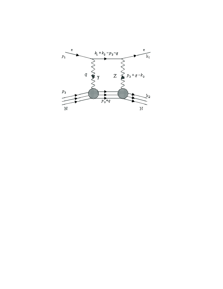
Figure 1: $\gamma-Z$ box diagram in the electron-nucleon scattering.

$$M^{\left\{\gamma-Z\right\}} = \frac{1}{16\pi^{4}}\int d^{4}q\left(i\overline{u}_{e}\Gamma_{\mu}^{Z-e}\frac{m_{e}+\not k_{1}+\not k_{2}-\not q-\not p_{2}}{\left(p_{2}-k_{1}-k_{2}+q\right)^{2}-m_{e}^{2}}\Gamma_{\nu}^{\gamma-e}u_{e}\right)$$

$$\ \ \left(i\overline{u}_{N}\Gamma_{\rho}^{Z-N}\frac{m_{N}+\not q+\not p_{2}}{\left(p_{2}+q\right)^{2}-m_{N}^{2}}\Gamma_{\alpha}^{\gamma-N}u_{N}\right)\left(\frac{g^{\nu\alpha}}{q^{2}}\frac{g^{\mu\rho}}{\left(p_{2}+q-k_{2}\right)^{2}-m_{Z}^{2}}\right).$$

In order to integrate the amplitude in Eq.(LABEL:e1.4) and the rest of the NLO loop integrals using FeynArts and FormCalc, it is necessary first to create a model file with declarations of all the fields participating in interaction and second to describe all the possible couplings of the fields on both generic and particle levels. For the case of electron-nucleon scattering, the only new particles in the model besides the particles of the Standard Model are neutron and proton, so it is rather straightforward to declare them in the FeynArts model file. On other hand, the description of the couplings according to the Eq.(4) and Eq.(5) in the FeynArts represents a certain problem. Because we use the monopole form factor approximation (see Eq.(8)), it introduces momentum dependence in the coupling’s denominator. For FeynArts to deal with momentum-dependent couplings with momentum dependence introduced in the denominator, these couplings have to be described as propagators. Of course, a propagator introduced in the coupling conflicts with the declaration of the fields in the FeynArts model files which use the same propagator notation. We can solve the problem by transferring the monopole form factor from the coupling part of model to the part where fields are described using propagator notation. For boxes that can be achieved by starting with the general definition of a four-point tensor integral of rank $k$ in the form

$$T_{\mu_{1}...\mu_{k}}^{4} = \frac{1}{i\pi^{2}}\int d^{4}q\frac{q_{\mu_{1}}...q_{\mu_{k}}}{\left(\left(p_{2}-k_{1}-k_{2}+q\right)^{2}-m_{e}^{2}\right)\left(\left(p_{2}+q\right)^{2}-m_{N}^{2}\right)}\cdot$$

$$\ \ \ \cdot\frac{1}{q^{2}}\cdot\frac{1}{\left(p_{2}+q-k_{2}\right)^{2}-m_{Z}^{2}}.$$

By adding the monopole form factor approximation into the above definition, we obtain a six-point tensor integral which can be reduced into a combination of four-point integrals by using the following expansion:

$$\frac{1}{D_{1}D_{2}}=\frac{1}{q^{2}}\cdot\frac{1}{\left(p_{2}+q-k_{2}\right)^{2}-m_{Z}^{2}}\cdot\frac{\Lambda^{4}}{\left(q^{2}-\Lambda^{2}\right)\left(\left(p_{2}+q-k_{2}\right)^{2}-\Lambda^{2}\right)}=$$

$$\ \ \ \frac{\Lambda^{2}}{\left(\Lambda^{2}-m_{Z}^{2}\right)}\left(\frac{1}{q^{2}-\Lambda^{2}}-\frac{1}{q^{2}}\right)\cdot\left(\frac{1}{\left(p_{2}+q-k_{2}\right)^{2}-\Lambda^{2}}-\frac{1}{\left(p_{2}+q-k_{2}\right)^{2}-m_{Z}^{2}}\right).$$

Here $\frac{1}{D_{1}D_{2}}$ represents the last two terms of the product in Eq.(LABEL:e1.19) multiplied by the two monopole form factors of the box diagram. Explicitly, the right-hand side of Eq.(LABEL:e1.20) can be written in the form

$$\frac{1}{D_{1}D_{2}}=\frac{\Lambda^{2}}{\left(\Lambda^{2}-m_{Z}^{2}\right)}\frac{1}{q^{2}}\frac{1}{\left(p_{2}+q-k_{2}\right)^{2}-m_{Z}^{2}}+\frac{-\Lambda^{2}}{\left(\Lambda^{2}-m_{Z}^{2}\right)}\frac{1}{q^{2}-\Lambda^{2}}\frac{1}{\left(p_{2}+q-k_{2}\right)^{2}-m_{Z}^{2}}+$$

$$\frac{-\Lambda^{2}}{\left(\Lambda^{2}-m_{Z}^{2}\right)}\frac{1}{q^{2}}\frac{1}{\left(p_{2}+q-k_{2}\right)^{2}-\Lambda^{2}}+\frac{\Lambda^{2}}{\left(\Lambda^{2}-m_{Z}^{2}\right)}\frac{1}{q^{2}-\Lambda^{2}}\frac{1}{\left(p_{2}+q-k_{2}\right)^{2}-\Lambda^{2}}$$ .

Substitution of the last equation into amplitude Eq.(LABEL:e1.4) results in an expansion where each term of the sum represents an amplitude constructed for electron-nucleon scattering with the point-like nucleon. Also, in this consideration, the couplings between nucleon and vector bosons are multiplied by the factor $\pm\sqrt{\frac{\Lambda^{2}}{\left(\Lambda^{2}-m_{Z}^{2}\right)}}$, and the structure of the second, third and fourth terms of Eq.(LABEL:e1.20a) suggests the introduction of fictitious vector boson particles $\left\{\delta\gamma,\delta Z\right\}$ with fixed masses $m_{\left\{\delta\gamma,\delta Z\right\}}=\Lambda$. These bosons have no physical meaning, of course, but they allow us to remove momentum dependence in the denominator of the coupling. Now we can model couplings between nucleon and vector fields using Eq.(4) and Eq.(5) with a monopole form factor moved into the definition of propagators for the new vector fields such as $\left\{\delta\gamma,\delta Z\right\}$ where $\Pi_{\left\{\delta\gamma,\delta Z\right\}}^{\mu\nu}=\frac{g^{\mu\nu}}{q^{2}-\Lambda^{2}}$. A diagrammatic representation of the proposed expansion is given by the set of Feynman graphs in Fig.(2).

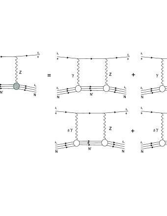
Figure 2: Expansion of the $\gamma-Z$ box in terms of $\delta\gamma,\,\delta Z$ particles

As for the boxes, we have all we need to complete the automated construction of amplitudes in the FeynArts and the calculations in the FormCalc. We should note that Eq.(LABEL:e1.4) is written for the $\left\{\gamma-Z\right\}$ box diagram only. To have a complete analysis, it is necessary to consider $\left\{Z-\gamma\right\}$, $\left\{\gamma-Z\right\}$ and $\left\{Z-\gamma\right\}$ crossed boxes as well. $\left\{Z-Z\right\}$ and $\left\{W-W\right\}$ box diagrams should be considered, too. Our calculations include 36 boxes in total.

II.4 Self-Energy Graphs

In total, 116 self-energy graphs and 6 counterterms contribute to the PV $\left\{e-N\right\}$ amplitude. This includes gauge and the gauge-fixing fields, the Higgs field, and virtual leptonic and quark pairs in creation-annihilation processes in the loops. Moreover, the vertex $\left\{N-V-N\right\}$ does not belong to the loop integrals and plays the role of a multiplicative factor proportional to the coupling defined in Eq.(4) and Eq.(5). In FormCalc the self-energy loop integrals can be evaluated using the expansion given in the Fig.(3), and then tensor decomposition and tensor reduction techniques applied, leaving the final result as a combination of one and two point scalar integrals which we compute using Gauss integration subroutines of LoopTools.

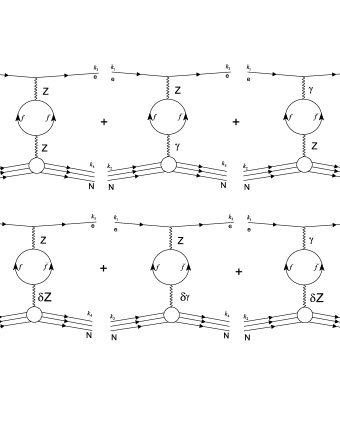
Figure 3: Expansion of the self-energy graphs in terms of $\delta\gamma,\,\delta Z$ partners. Here, factor $\pm\sqrt{\frac{\Lambda^{2}}{\left(\Lambda^{2}-m_{Z}^{2}\right)}}$ used for the couplings of the box diagrams should be replaced by one.

To cancel ultraviolet divergences we employ an on-shell renormalization scheme according to (Hah97, ). We have to assume that quarks in the self-energy loops are free, but it places certain constraints. Since quarks are confined, a QCD strong quark-quark interaction should always be considered. It is possible to bypass these complications by replacing quarks with pions, or use “free” quarks but with adjusted effective masses. Here, we use the second approach with the effective mass of the quarks coming from a fit of hadronic vacuum polarization to the measurements of QED cross section of the process $e^{+}e^{-}\rightarrow\,$hadrons normalized to the QED $e^{+}e^{-}\rightarrow\mu^{+}\mu^{-}$ cross section. The real part of the renormalized hadronic vacuum polarization satisfies the dispersion relation:

$$\bigtriangleup\alpha_{hadr}^{\gamma}\left(s\right)=-Re\widehat{\,\Pi}_{had}^{\gamma}\left(s\right)=\frac{\alpha}{3\pi}s\int_{4m_{\pi}^{2}}^{\infty}\frac{R^{\gamma}\left(s^{\prime}\right)}{s^{\prime}\left(s^{\prime}-s\right)}ds^{\prime},$$ (15)

with

$$R^{\gamma}\left(s\right)=\frac{\sigma\left(e^{+}e^{-}\rightarrow hadrons\right)}{\sigma\left(e^{+}e^{-}\rightarrow\mu^{+}\mu^{-}\right)}$$ (16)

being a very well known experimental quantity and used here as an input parameter.

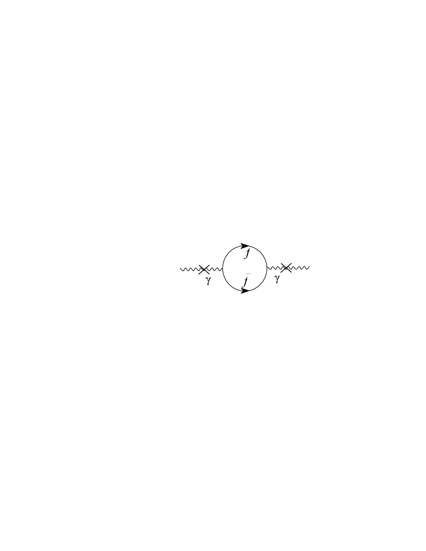
Figure 4: Truncated self-energy graph in hadronic vacuum polarization

Hadronic vacuum polarization $\widehat{\Pi}_{had}^{\gamma}\left(s\right)$ is related to the truncated $\left\{\gamma-\gamma\right\}$ renormalized self-energy (See Fig.(4)) by the following expression:

$$\widehat{\sum}_{ferm}^{\gamma}\left(s\right)=s\widehat{\Pi}_{had}^{\gamma}\left(s\right)+i\,Im\left(\widehat{\sum}_{ferm}^{\gamma}\left(s\right)\right),$$ (17)

which can be easily evaluated by employing the free quark approximation. An updated value of the dispersion integral, along with a logarithmic parametrization, can be taken from (Burkhardt2001, ). A new reported value coming from the light quark contribution at $s=m_{Z}^{2}$ is $\bigtriangleup\alpha_{hadr}^{\gamma(5)}\left(m_{Z}^{2}\right)=-0.02761$. This value can be reproduced by Eq.(17) using the following masses of the light quarks: $m_{u}=m_{d}=53\,MeV$ (corresponds to $\bigtriangleup\alpha_{hadr}^{\gamma(5)}\left(m_{Z}^{2}\right)=-0.027609$). Clearly, the values of the light quark masses at low-Q scattering processes should be adjusted by using this approach, but with $\bigtriangleup\alpha_{hadr}^{\gamma(5)}\left(s\right)$ calculated in the region of $\sqrt{s}<4.0$ GeV. The simple logarithmic parametrization can be used here to extract quark masses at low momentum transfer:

$$\bigtriangleup\alpha_{hadr}^{\gamma(5)}\left(s\right)=A+B\ln\left(1+C\cdot s\right),$$ (18)

with $A,B$ and $C$ parameters taken from (Burkhardt2001, ). For low-momentum transfer experiments, the c.m.s. energy is $\sqrt{s}<4.0$ $GeV$, which gives, $m_{u}=m_{d}\simeq 45\,MeV$.

II.5 Vertex Corrections Graphs

The vertex correction contributions can be split into two classes. In the first class, where the electron vertex is at the one-loop level, the amplitude is calculated according to (BAB2002, ). As in the case of the self-energy graphs, the hadronic vertex does not belong to the loop integrals, and therefore the PV amplitude is constructed according to the SM Feynman rules employed in the FeynArts package. Generally, the electron vertex corrections have an infrared divergence at $q\rightarrow 0$ and are treated by the bremsstrahlung contribution considered in (ThesisAA, ).

The second class of the triangle graphs are hadronic vertex corrections. In this case, to evaluate the amplitude automatically using the packages FeynArts and FormCalc, we construct an expansion similar to that given for the box diagrams. To work out the set of rules for the triangle topology, it is sufficient to consider the example in Fig.(5).

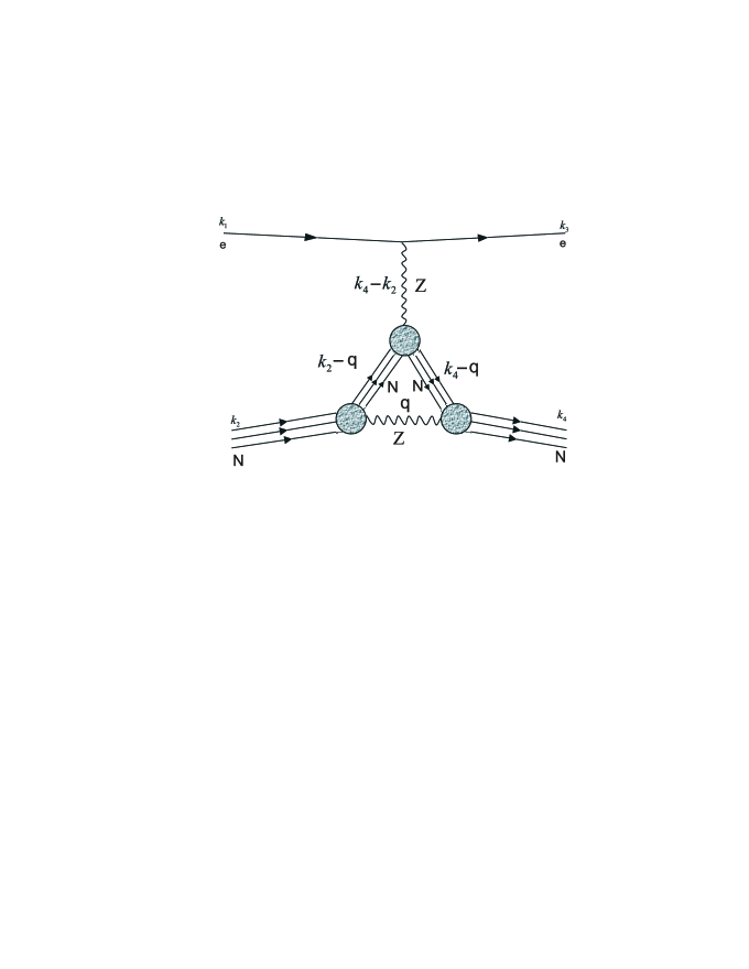
Figure 5: Hadronic vertex correction graph.

For the graph in Fig.(5), the amplitude denominator has the structure

$$\frac{1}{D_{1}D_{2}D_{3}D_{4}} = \frac{1}{\left(k_{4}-q\right)^{2}-m_{N}^{2}}\cdot\frac{1}{\left(k_{2}-q\right)^{2}-m_{N}^{2}}\cdot\frac{1}{\left(k_{4}-k_{2}\right)^{2}-m_{Z}^{2}}\cdot$$

$$\ \ \ \ \ \ \frac{1}{q^{2}-m_{Z}^{2}}\cdot\ \frac{\Lambda^{2}}{\left(k_{4}-k_{2}\right)^{2}-\Lambda^{2}}\cdot\frac{\Lambda^{4}}{\left(q^{2}-\Lambda^{2}\right)^{2}},$$

which can be easily expanded into

$$\frac{1}{D_{1}D_{2}D_{3}D_{4}} = \frac{1}{\left(k_{4}-q\right)^{2}-m_{N}^{2}}\frac{1}{\left(k_{2}-q\right)^{2}-m_{N}^{2}}\cdot$$

$$\ \ \ \ \ \ \ \left(\frac{B^{Z-N}}{\left(k_{4}-k_{2}\right)^{2}-m_{Z}^{2}}+\frac{B^{\delta Z-N}}{\left(k_{4}-k_{2}\right)^{2}-\Lambda^{2}}\right)\cdot$$

$$\ \ \ \ \ \ \ \lim_{\left\{\Lambda_{1},\Lambda_{2}\right\}\rightarrow\Lambda}\ \left(\frac{\left(C^{Z-N}\right)^{2}}{q^{2}-m_{Z}^{2}}+\frac{\left(C^{\delta_{1}Z-N}\right)^{2}}{q^{2}-\Lambda_{1}^{2}}+\frac{\left(C^{\delta_{2}Z-N}\right)^{2}}{q^{2}-\Lambda_{2}^{2}}\right).$$

Here, the coefficients $B^{Z-N}$ and $B^{\delta Z-N}$ are equal to $\pm\sqrt{\frac{\Lambda^{2}}{\left(\Lambda^{2}-m_{Z}^{2}\right)}}$ respectively. $C^{Z-N},C^{\delta_{1}Z-\Lambda_{1}}$, and $C^{\delta_{2}Z-\Lambda_{2}}$ can be calculated using the following formulae:

$$\left(C^{Z-N}\right)^{2} = \frac{\Lambda^{4}}{\left(m_{Z}^{2}-\Lambda_{1}^{2}\right)\left(m_{Z}^{2}-\Lambda_{2}^{2}\right)},$$

$$\left(C^{\delta_{1}Z-N}\right)^{2} = -\frac{\Lambda^{4}}{m_{Z}^{2}-\Lambda_{1}^{2}}\frac{1}{\Lambda_{1}^{2}-\Lambda_{2}^{2}},$$

$$\left(C^{\delta_{2}Z-N}\right)^{2} = -\frac{\Lambda^{4}}{m_{Z}^{2}-\Lambda_{1}^{2}}\left(\frac{1}{m_{Z}^{2}-\Lambda_{2}^{2}}-\frac{1}{\Lambda_{1}^{2}-\Lambda_{2}^{2}}\right).$$

The expansion of the amplitude denominator in Eq.(LABEL:e1.35) has a simple graphical representation (see Fig.(6)) and suggests, in this particular case of the triangle topology, that a set of virtual particles $\delta_{1}Z$ and $\delta_{2}Z$ should be introduced in the NLO hadronic vertex corrections.

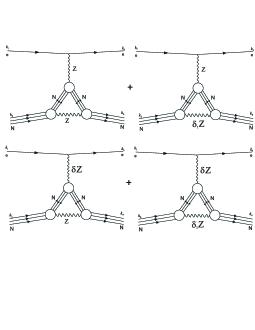
Figure 6: Hadronic vertex expansion in the terms of $Z,\,\delta_{1}Z$ and $\delta_{2}Z$ partners.

Although ultraviolet divergences are absent in the hadronic vertex corrections due to the additional terms proportional to $\frac{\Lambda^{2}}{q^{2}-\Lambda^{2}}$ in the coupling, it is still necessary to compute the wave function renormalization with some details given in the appendix. As well as in the case of electron vertex corrections, the nucleon vertex will have an infrared divergence at the pole $q\rightarrow 0$ (for the proton). A detailed discussion of the treatment of this type of divergence is given in (ThesisAA, ).

III Numerical Results and Conclusions

The application of the methods described above for $\left\{e-N\right\}$ scattering can be found in calculations of the weak charges of the nuclei. Consider the parity-violating Hamiltonian in Eq.(9). Here, for a heavy nucleus we have a coherent effect for $V\left(N\right)\otimes A\left(e\right)$:

$$\left(\overline{u}_{N}\gamma^{\mu}u_{N}\right)\rightarrow\rho_{nuc}\left(r\right)\delta_{\mu,0}.$$ (22)

The contribution coming from $V\left(e\right)\otimes A\left(N\right)$ is small as it depends on unpaired valence nucleons. The latter determines the Hamiltonian for the electron parity-violating interaction with the nucleus in the following form:

$$H\left(r\right)=\frac{G_{\mu}}{2\sqrt{2}}Q_{weak}\gamma_{5}\rho_{nuc}\left(r\right).$$ (23)

A relation between the weak charge $Q_{weak}$ and form factors $\left\{C_{1p},C_{1n}\right\}$ is straightforward:

$$Q_{weak}^{p} = 2C_{1p}\left(Q^{2}\rightarrow 0\,GeV^{2}\right),$$

$$Q_{weak}^{n} = 2C_{1n}\left(Q^{2}\rightarrow 0\,GeV^{2}\right).$$

If we take into account only the leading order of the interaction, the weak charge of the proton and neutron have the simple definitions:

$$Q_{weak}^{p\left(0\right)} = 1-4s_{w}^{2},$$

$$Q_{weak}^{n\left(0\right)} = -1,$$

and for the nucleus

$$Q_{weak}=Z\cdot Q_{weak}^{p}+N\cdot Q_{weak}^{n},$$ (26)

where $Q_{weak}^{p},$ $Q_{weak}^{n}$ are the weak charges of the proton and neutron including NLO corrections.

As one can see from Fig.(7), the input of the NLO corrections is much more significant for the proton than for the neutron. This makes experiments involving neutrons more interesting, as they allow for the cleaner weak charge extraction.

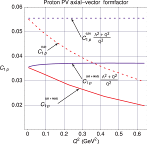
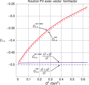
Figure 7: Momentum transfer dependence of the form factors $\left\{C_{1p},\,C_{1n}\right\}$ and $\left\{C_{1p},\,C_{1n}\right\}\cdot\frac{\Lambda^{2}+Q^{2}}{Q^{2}}$. The dotted line represents parity-violating form factor at the tree-level (LO) only, and the solid line shows the result with NLO contribution included (LO+NLO).

Also, form factors $C_{1p}$ and $C_{1n}$ normalized by the monopole term $\frac{\Lambda^{2}}{\Lambda^{2}+Q^{2}}$ (see Fig.(7)) do not exhibit strong momentum transfer dependence and hence are model independent. This justifies to some extent our choice of the monopole form factor approximation.

Extrapolation of the $C_{1p}$ and $C_{1n}$ to zero momentum transfer point (see Fig.(7)) gives: $C_{1p}=0.0360\pm 0.0005$ and $C_{1n}=-0.4950\pm 0.0020$. The most important of these numbers is the result for $C_{1p}.$ It has been evaluated most recently in (EKM2003, ), leading to $C_{1p}=0.0358\pm 0.0003$.

The available results from atomic parity-violating experiments for the weak charges of $Cs_{55}^{133},\,Tl_{81}^{205}$ and $Bi_{83}^{209}$ ((L2003, ) and references within, and (BZ78, )) can be used as an experimental test of the theoretical predictions:

$$Cs_{55}^{133}(\exp) = -72.65\pm 0.28\pm 0.34,$$

$$Tl_{81}^{205}(\exp) = -114.8\pm 1.2\pm 3.4,$$

$$Bi_{83}^{209}(\exp) = -140\pm 40.$$

Here, the errors are statistical, systematic and coming from an uncertainty of the atomic-physics theory, respectively. For example, in the case of $Cs_{55}^{133},$ one should observe $7s\;(excited)\rightarrow 6s\;(ground)$ parity-violating electric dipole transitions in order to extract the weak charge of $Cs_{55}^{133}.$ This requires an accurate knowledge of the atomic wave functions. Some of the analysis of the issues involved, with an extensive reference list, is given in (PDG, ) and (EKM2003, ). Using Eq.(LABEL:d1.3) and Eq.(26) we compute the following results for the corresponding nuclear weak charges:

$$Cs_{55}^{133}(\mathrm{theory}) = -73.26\pm 0.26,$$

$$Tl_{81}^{205}(\mathrm{theory}) = -114.9\pm 0.4,$$

$$Bi_{83}^{209}(\mathrm{theory}) = -118.8\pm 0.4,$$

which clearly agree with the experiment. The theoretical uncertainty is estimated quite generously and comes mostly from the numerical integration and the extrapolation to the zero momentum transfer point. Although the NLO corrections contribute only $\sim 1.5\%$ to the results in Eq.(LABEL:d1.7a), their value is still about four times larger than our theoretical uncertainty. Thus, the more precise is the experiment (like $Cs_{55}^{133}$), the more important it becomes to evaluate most carefully the full set of the applicable NLO corrections. Although our model predictions for the nuclear weak charges are in good agreement with the available experimental results, to allow more definitive conclusions about the validity of the proposed computational model, the experimental errors for precision measurements of the weak charge of the nucleon will have to be reduced.

Any significant deviation of the weak charge of the proton from the Standard Model prediction at low $Q^{2}$ would be a signal of new physics. The proton’s weak charge $Q_{weak}^{p}$ is a well-defined experimental observable. At $Q^{2}\rightarrow 0$ the asymmetry can be parametrized as

$$\mathcal{A}=\left[\frac{-G_{F}Q^{2}}{4\sqrt{2}\pi\alpha}\right][Q^{2}Q_{weak}^{p}+Q^{4}B(Q^{2})],$$

where $B(Q^{2})$ is a function of Sachs electromagnetic form factors $G_{E,M}^{\gamma}$ related to the Dirac and Pauli form factors by the following expression:

$$G_{E}^{\gamma}=F_{1}-\frac{Q^{2}}{4m_{N}^{2}}F_{2},\,\,\,G_{M}^{\gamma}=F_{1}+F_{2}.$$ (29)

The measurement of $Q_{weak}^{p}$ will be done by the $Q_{weak}$ collaboration (Qweak, ), and may have extremely interesting physical implications. See, for example, (EKM2003, ). It will allow one to determine the proton’s weak charge with $\simeq$4% combined statistical and systematic errors, which leads to $9\sigma$ for the running of the weak mixing angle. The Standard Model evolution predicts a shift of $\Delta sin^{2}\theta_{W}=+0.007$ at low $Q^{2}$ with respect to the $Z^{0}$ pole best fit value of $0.23113\pm 0.00015.$ The weak mixing angle at the energy scale close to the $Z^{0}$ pole was measured very precisely, but a precision experimental study of the evolution of $sin^{2}\theta_{W}$ to lower energies still has to be carried out. The asymmetry measurements proposed for $Q_{weak}$ experiment will go as low as $Q^{2}=0.03\,GeV^{2}$, making it a very competitive experiment.

Using the Dirac and Pauli form factors, we can now compute the extensive set of one-loop hadronic electroweak NLO corrections along with the weak charges of the proton and neutron. Using a monopole approximation for the form factors, we modified general electroweak couplings by inserting the appropriate form factors into the vertices. The monopole structure of the form factors allows us to substitute one Feynman diagram with “structured” nucleon with a set of diagrams involving only point-like nucleon. This expansion can be visualized by adding fictitious additional vector bosons of mass $\Lambda$. For renormalization, we choose the on-shell renormalization scheme.

In conclusion, it is evident that computational symbolic packages such as FeynArts and FormCalc can be efficiently adapted for the theoretical evaluation of NLO effects in electron-nucleon scattering. Refs (ABB2005_a, ) and (ABB2006, ) give some additional details. A newly proposed measurement of the electron weak charge in parity-violating Moller scattering at 12 GeV at JLab could be a very interesting challenge, for example.

IV Appendix

IV.1 Some analytical details on couplings

To introduce couplings between vector bosons and nucleon into the model files of FeynArts, instead of vector and axial-vector representation, we employ use of chirality projectors. That can be achieved if we compare Eq.(1), Eq.(2) with Eq.(5), combined with Eq.(6) and Eq.(7), then it is possible to write

$$\Gamma_{\mu}^{Z-N}\left(q\right)=ie[\frac{g_{R}^{Z-N}\left(q\right)+g_{L}^{Z-N}\left(q\right)}{2}\gamma_{\mu}+\frac{g_{R}^{Z-N}\left(q\right)-g_{L}^{Z-N}\left(q\right)}{2}\gamma_{\mu}\gamma_{5}+$$

$$+\frac{i}{2m_{N}}\sigma_{\mu\alpha}q^{\alpha}f_{2}\left(q\right)] =$$

$$=ie\left[g_{L}^{Z-N}\left(q\right)\gamma_{\mu}\varpi_{-}+g_{R}^{Z-N}\left(q\right)\gamma_{\mu}\varpi_{+}+\frac{i}{2m_{N}}\sigma_{\mu\alpha}q^{\alpha}f_{2}\left(q\right)\right]$$

$$\Gamma_{\mu}^{\gamma-N}\left(q\right)=ie\left[\frac{g_{L}^{\gamma-N}\left(q\right)+g_{R}^{\gamma-N}\left(q\right)}{2}\gamma_{\mu}+\frac{i}{2m_{N}}\sigma_{\mu\alpha}q^{\alpha}F_{2}\left(q\right)\right]=$$

$$=ie\left[g_{L}^{\gamma-N}\left(q\right)\gamma_{\mu}\varpi_{-}+g_{R}^{\gamma-N}\left(q\right)\gamma_{\mu}\varpi_{+}+\frac{i}{2m_{N}}\sigma_{\mu\alpha}q^{\alpha}F_{2}\left(q\right)\right],$$

where

$$g_{L,R}^{Z-N}\left(q\right) = \frac{1}{4c_{w}s_{w}}\left(F_{1}^{V\left(N\right)}\left(0\right)-4s^{2}F_{1}\left(0\right)\pm g_{A}\left(0\right)\right)\frac{\Lambda^{2}}{\Lambda^{2}-q^{2}},$$

$$g_{L,R}^{\gamma-N}\left(q\right) = g^{\gamma-N}\left(q\right)=F_{1}\left(0\right)\frac{\Lambda^{2}}{\Lambda^{2}-q^{2}}.$$

In Eqs.(LABEL:e1.11) and (LABEL:e1.12), we have adopted the general structure of the coupling from Eq.(1), with coupling strengths $g_{L,R}^{Z-N}\left(q\right)$ and $g_{L,R}^{\gamma-N}\left(q\right)$ given by Eq.(LABEL:e1.13). Vector part of the coupling $\sigma_{\mu\alpha}q^{\alpha}$ also can be replaced by the chirality projectors $\omega_{\pm}$ in the following way

$$\sigma_{\mu\alpha}q^{\alpha} = \frac{i}{2}\left(\left[\gamma_{\mu},\not q\right]\varpi_{-}+\left[\gamma_{\mu},\not q\right]\varpi_{+}\right).$$ (33)

Moreover, to adopt FeynArts representation of the coupling through the product of generic and class type of the couplings, we introduce the following matrix representation of Eq.(LABEL:e1.11) and Eq.(LABEL:e1.12):

$$\Gamma\left(N,N,V_{\mu}\right)=\left(\begin{tabular}[]{llll}$\gamma_{\mu}\varpi_{-}$,&$\gamma_{\mu}\varpi_{+}$,&$\left[\gamma_{\mu},\not q\right]\varpi_{-}$,&$\left[\gamma_{\mu},\not q\right]\varpi_{+}$\end{tabular}\right)\overrightarrow{G}_{NNV}\left(q\right),$$ (34)

with $\overrightarrow{G}_{NNV}$ defines coupling between classes of the vector bosons and nucleons and expressed as a $2\times 4$ matrix

$$\overrightarrow{G}_{NNV}=ie\left(\begin{array}[]{cc}g_{L}^{V-N}\left(q\right)&G_{1L}^{V-N}\\ g_{R}^{V-N}\left(q\right)&G_{1R}^{V-N}\\ -\frac{1}{4m_{N}}F_{2}^{V-N}\left(q\right)&G_{2L}^{V-N}\\ -\frac{1}{4m_{N}}F_{2}^{V-N}\left(q\right)&G_{2R}^{V-N}\end{array}\right).$$ (35)

The second column of $\overrightarrow{G}_{NNV}$ represents counterterms of the first order. The Pauli form factor $F_{2}^{V-N}$ in Eq.(35) has the following structure:

$$F_{2}^{Z-N}\left(q\right) = f_{2}\left(q\right),$$

$$F_{2}^{\gamma-N}\left(q\right) = F_{2}\left(q\right).$$

The coupling defined in Eq.(35) has a counterterm part at the one-loop level represented by the matrix, which has following structure:

$$\left(\begin{array}[]{c}G_{1L}^{V-N}\\ G_{1R}^{V-N}\\ G_{2L}^{V-N}\\ G_{2R}^{V-N}\end{array}\right)=\left(\begin{array}[]{c}g_{L}^{V-N}Re[\delta\,f_{L}]\\ g_{R}^{V-N}Re[\delta\,f_{R}]\\ -\frac{1}{4m_{N}}F_{2}^{V-N}\left(q\right)Re[\delta\,f_{L}]\\ -\frac{1}{4m_{N}}F_{2}^{V-N}\left(q\right)Re[\delta\,f_{R}]\end{array}\right),$$ (37)

where the hadronic field renormalization constants $\delta\,f_{L,R}$ are computed using the expansion on Fig.(8). More details are given in Ref.(ThesisAA, ).

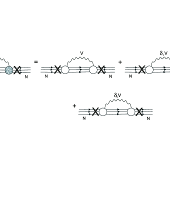
Figure 8: Hadronic wave function renormalization expansion.

References

- (1) W. J. Marciano, A. Sirlin, Phys. Rev. D, 29, 75 (1984).
- (2) J. Erler, A. Kurylov, M. J. Ramsey-Musolf, Phys. Rev. D68, 016006 (2003).
- (3) T. Hahn, arXiv:hep-ph/0012260v2.
- (4) T. Hahn, M. Perez-Victoria, arXiv:hep-ph/9807565v1.
- (5) T. Hahn, M. Perez-Victoria, Comput. Phys. Commun. 118 (1999) 153 [hep-ph/9807565].
- (6) G. J. van Oldenborgh, Z. Phys. C46 (1990) 425.
- (7) J. A. M. Vermaseren, math-ph/0010025.
- (8) S. Barkanova, A. Aleksejevs, P. Blunden, Jefferson Laboratory preprint #JLAB-THY-02-59, and nucl-th/0212105, (2002).
- (9) A. Aleksejevs, PhD Thesis, University of Manitoba (2005).
- (10) S. Barkanova, PhD Thesis, University of Manitoba (2004).
- (11) M. Bohm, H. Speisberger, W. Hollik, Fort. Phys., 34, 688 (1986).
- (12) T. Hahn, Ph.D. thesis, University of Karlsruhe, (1997).
- (13) H. Burhardt, B. Pietzyk, Phys. Lett. B, 513, 46 (2001).
- (14) Paul Langacker, J. Phys. G29, 35-48 (2003).
- (15) L. Barkov and M. Zolotorev, Pisma Zh. Eksp. Teor. Fiz. 27, 379 (1978).
- (16) Particle Data Group, W.-M. Yao et al., Journal of Physics G 33, 1 (2006).
- (17) J. Bowman, R. Carlini, J. Finn, V. A. Kowalski, S. Page, Jefferson Lab Experiment, E02020, Proposal to PAC 21 at http://www.jlab.org/qweak/.
- (18) A. Aleksejevs, S. Barkanova, P. Blunden, proceedings of LP2005, June 30 - July 5, Uppsala, Sweden, 2005.
- (19) A. Aleksejevs, S. Barkanova, P. Blunden and N. Deg, arXiv:0707.0657 (2007).