Energy-dependent Lorentz covariant parameterization
of the NN interaction between 50 and 200 MeV

Abstract

For laboratory kinetic energies between 50 and 200 MeV, we focus on generating an energy-dependent Lorentz covariant parameterization of the on-shell nucleon-nucleon (NN) scattering amplitudes in terms of a number of Yukawa-type meson exchanges in first-order Born approximation. This parameterization provides a good description of NN scattering observables in the energy range of interest, and can also be successfully extrapolated to energies between 40 and 300 MeV.

I Introduction

We present an energy-dependent Lorentz covariant parameterization of the on-shell nucleon-nucleon (NN) scattering matrix at incident laboratory kinetic energies ranging from 50 to 200 MeV. In particular, we focus on the relativistic Horowitz-Love-Franey (HLF) model Ho85 ; Mu87 ; Ma96 ; Ma98 which parameterizes the NN scattering amplitudes as a number of Yukawa-type meson-exchange terms.

The original HLF model parameterized $pp$ and $pn$ scattering amplitudes at discrete energies of 135, 200 and 400 MeV Ho85 ; Mu87 . A drawback of the initial representation was that separate fits were performed at each energy resulting in non-systematic and unphysical trends in the various model parameters as a function of energy. This was also undesirable in the sense that it hindered meaningful comparisons of the off-shell properties of the NN scattering matrix at different energies. This problem was subsequently addressed by Maxwell who developed energy-dependent parameterizations of the NN scattering amplitudes for two energy ranges, namely 200 - 500 MeV Ma96 and 500 - 800 MeV Ma98 . Since several experiments at future radioactive ion beam facilities will be conducted at nucleon energies lower than 200 MeV, it is essential to extend the HLF model to lower energies so as to generate reliable input for nuclear reaction models.

An attractive feature of HLF model is the existence of a simple relationship – lacking in conventional nonrelativistic models – between the Lorentz invariant NN scattering amplitudes and mesons mediating the interaction. Moreover, this model has a physical basis in the one-boson-exchange (OBE) picture, since the values of the real meson-nucleon coupling constants (at energies higher than 200 MeV) are similar to those arising from more sophisticated OBE models Ho85 . In addition to being employed as the basic NN interaction driving the dominant reaction mechanism in several relativistic scattering models of nucleon-induced reactions, the HLF model has also been applied to extract relativistic microscopic optical potentials Mu87 ; No05 ; Ma98b ; Co05 for studying elastic proton scattering from stable nuclei, as well as for generating scattering wave functions for evaluating transition matrix elements in various relativistic distorted wave models Ma98b ; No05 . More specifically, the latter microscopic optical potentials are generated by folding the HLF $t$-matrix with the relevant relativistic mean field Lorentz densities via the so-called $t\rho$-approximation. Indeed, one of the triumphs of this folding procedure is that the microscopic potentials, for energies from 200 to 400 MeV, are virtually identical to the corresponding global phenomenological Dirac optical potentials, which have been shown to provide excellent quantitative predictions of scattering observables for elastic proton scattering from spin-zero stable nuclei ranging from ¹²C to ²⁰⁸Pb and for incident energies between 20 and 1040 MeV Co93 .

One of the frontier areas of research in nuclear physics is to understand the properties of nuclei far from the beta-stability line, the so-called exotic or unstable nuclei. These studies provide insight into the nuclear processes that underlie the evolution of the stars and the origin of the elements in the cosmos. Indeed, a number of radioactive ion beam facilities are currently under construction to study short-lived rare isotopes. In particular, there are plans to study exclusive proton-induced proton-knockout reactions (using inverse kinematics) at facilities such as RIKEN and GSI for both neutron- and proton-rich nuclei at energies lower than 200 MeV per nucleon. For the eventual interpretation of these data it is essential to have reliable optical potentials. Existing global Dirac optical potentials have been constrained to reproduce elastic proton scattering from stable nuclei Co93 , and hence there is no reason to believe that these potentials can be reliably extrapolated for studies of unstable nuclei. On the other hand, one can readily extend the above-mentioned folding procedure to calculate scattering potentials for proton-induced reactions on exotic nuclei. Moreover, the successful application of the relativistic $t\rho$ approximation to describe elastic proton scattering from stable nuclei, gives one confidence in extending this approach to study proton scattering on exotic nuclei. Two basic ingredients underly the realization of these folding potentials, namely a suitable analytical representation for the NN interaction in the energy range of interest, as well as an appropriate relativistic model of nuclear structure Me06 . Several relativistic mean field nuclear structure models are currently being developed for studying the structure of unstable nuclei To03 ; Me06 . In this paper, however, we focus on developing a HLF-type parameterization of the NN scattering amplitudes at energies lower than 200 MeV. The generation of the corresponding microscopic optical potentials will be considered in a future paper, in which Pauli blocking corrections and nuclear medium modifications to the NN interaction are expected to be significant and will be taken into account Mu87 ; De00 ; De05 .

The HLF model is described in Sec. (II). The fitting procedure and corresponding results are presented in Secs. (III) and (IV), respectively.

II The relativistic Horowitz-Love-Franey model

The most general parametrization of the nonrelativistic on-shell elastic NN scattering matrix – consistent with rotational, parity, time-reversal and isospin invariance – is completely determined by five complex scattering amplitudes. Depending on the specific application of interest, the NN scattering matrix can be recast into several distinct, but equivalent, five-term representations, one of which is the so-called Bystricky parameterization By78 , namely:

$$(2ik)^{-1}\hat{f}_{\rm{cm}}(\vec{k},\vec{k}^{\prime}) = \frac{1}{2}\{(a+b)I_{1}\otimes I_{2}+(a-b)({\vec{\sigma}_{1}}\otimes I_{2})\cdot{\hat{n}}(I_{1}\otimes{\vec{\sigma}_{2}})\cdot{\hat{n}}+(c+d)$$ (1)

$$\times ({\vec{\sigma}_{1}}\otimes I_{2})\cdot{\hat{m}}(I_{1}\otimes{\vec{\sigma}_{2}})\cdot{\hat{m}}+(c-d)({\vec{\sigma}_{1}}\otimes I_{2})\cdot{\hat{\ell}}(I_{1}\otimes{\vec{\sigma}_{2}})\cdot{\hat{\ell}}$$

$$+ e({\vec{\sigma}_{1}}\otimes I_{2}+I_{1}\otimes{\vec{\sigma}_{2}})\cdot{\hat{n}}\}$$

where $\otimes$ denotes a kronecker product, $\vec{\sigma}_{1}$ and $\vec{\sigma}_{2}$ refer to the usual Pauli spin matrices associated with the projectile and target nucleons, 1 and 2 respectively, $I_{1}$ and $I_{2}$ are the respective $2\times 2$ unit matrices, and the basis vectors $\hat{\ell}$, $\hat{m}$ and $\hat{n}$ are defined as:

$$\begin{array}[]{lll}{\hat{\ell}}\ =\ \frac{\vec{k}^{\prime}\ +\ \vec{k}}{|\vec{k}^{\prime}\ +\ \vec{k}|},&{\hat{m}}\ =\ \frac{\vec{k}^{\prime}\ -\ \vec{k}}{|\vec{k}^{\prime}\ -\ \vec{k}|},&{\hat{n}}\ =\ \frac{\vec{k}\ \times\ \vec{k}^{\prime}}{|\vec{k}\ \times\ \vec{k}^{\prime}|}\end{array}\;,$$ (2)

where ${\vec{k}}$ and ${\vec{k}^{\prime}}$ are the initial and final momenta of the interacting nucleons in the NN centre-of-mass frame. The scattering matrix is normalized such that the polarized differential cross section for free NN scattering is given by

$$(\frac{d\sigma}{d\Omega})_{\rm{pol}}\ =\ |\langle{\chi}^{\dagger}_{{s^{\prime}}_{1}}{\chi}^{\dagger}_{{s^{\prime}}_{2}}|\hat{f}_{\rm{cm}}|{\chi}_{{s}_{1}}{\chi}_{{s}_{2}}\rangle|^{2}$$ (3)

where the $\chi$’s represent the usual Pauli spinors.

For relativistic applications, the preceding nonrelativistic phenomenology, expressed by Eq. (1), can be cast into many different relativistic Lorentz invariant forms of which the on-shell NN matrix elements are identical to those of the nonrelativistic scattering matrix. A convenient choice of the relativistic NN scattering matrix, commonly referred to as the IA1 representation and originally proposed by McNeil, Ray and Wallace Mc83 , is given by:

$$\hat{t}_{NN}=\sum_{L=1}^{5}F_{L}(s,t,u)\lambda_{L}^{(1)}\cdot\lambda_{L}^{(2)}$$ (4)

where $s$, $t$ and $u$ quantities denote the usual Mandelstam variables, $s\equiv(k_{1}+k_{2})^{2}$, $t\equiv(k_{1}-k^{\prime}_{1})^{2}$, where $u\equiv(k_{1}-k^{\prime}_{2})^{2}$, and $k_{1}\equiv(E,\vec{k})$ and $k_{2}\equiv(E,-\vec{k})$ define the incident 4-momenta of the projectile and target nucleons respectively in the center-of-mass frame, with similar definitions holding for the outgoing (primed) nucleons. The $L^{\rm{,s}}$ index the five Dirac matrices listed in Table 1, and the dot product implies contraction of the Lorentz indices.

Table 1: Dirac matrix types parameterizing the free NN amplitudes.

L	Lorentz type	Dirac matrices
1	Scalar (S)	$I_{4\times 4}$
2	Vector (V)	$\gamma_{\mu}$
3	Pseudoscalar (P)	$\gamma_{5}$
4	Axial-vector (A)	$\gamma_{5}\gamma_{\mu}$
5	Tensor (T)	$\sigma_{\mu\nu}$

The transformation between the nonrelativistic on-shell NN $a$, $b$, $c$, $d$, $e$ amplitudes and the relativistic $F_{S}$, $F_{V}$, $F_{P}$, $F_{A}$, $F_{T}$ amplitudes is readily established by equating the matrix elements of the nonrelativistic scattering matrix, given by Eq. (1), to the matrix elements of the relativistic scattering matrix, given by Eq. (4) Ho85 ; Mu87 ; Ma96 ; Ma98 , namely:

$$(2ik)^{-1}\chi^{\dagger}_{s^{\prime}_{1}}\chi^{\dagger}_{s^{\prime}_{2}}\hat{f}_{cm}\chi_{s_{1}}\chi_{s_{2}}\ =\ \bar{u}(k^{\prime}_{1},s^{\prime}_{1})\bar{u}(k^{\prime}_{2},s^{\prime}_{2})\hat{t}_{NN}u(k_{1},s_{1})u(k_{2},s_{2})\;,$$ (5)

where the Dirac spinors $u$ are normalized such that $\bar{u}u=1$. The corresponding $5\times 5$ matrix ${\cal O}_{5\times 5}$ linking the two representations is given by

$$\left(\begin{array}[]{c}a\\ b\\ c\\ d\\ e\\ \end{array}\right)=ik{\cal O}_{5\times 5}\left(\begin{array}[]{c}F_{S}\\ F_{V}\\ F_{P}\\ F_{A}\\ F_{T}\\ \end{array}\right)$$ (16)

where

$${\cal O}_{5\times 5}=\left(\begin{array}[]{ccccc}\cos\theta&\cos\theta&\cos\theta&-\cos\theta&-4\sin\theta\\ 1&-1&1&1&0\\ -1&1&1&1&0\\ 1&1&-1&1&0\\ -i\sin\theta&-i\sin\theta&-i\sin\theta&i\sin\theta&-4i\cos\theta\\ \end{array}\right)\left(\begin{array}[]{ccccc}\alpha&e\alpha+p\beta&0&p\alpha+e\beta&-2\beta\\ -e\gamma&-\gamma&-p\gamma&-\delta&2(p+e)\delta\\ \alpha&(p+e)\alpha&0&(e-p)\alpha&2\alpha\\ e\gamma&\gamma&-p\gamma&-\gamma&2\gamma\\ -\epsilon&-\epsilon&0&\epsilon&-2\epsilon\\ \end{array}\right)$$ (27)

and

$$\alpha = \cos^{2}\frac{\theta}{2}$$

$$\beta = 1+\sin^{2}\frac{\theta}{2}$$

$$\gamma = \sin^{2}\frac{\theta}{2}$$

$$\delta = 1+\cos^{2}\frac{\theta}{2}$$

$$\epsilon = \frac{E}{M}\sin\frac{\theta}{2}\cos\frac{\theta}{2}$$

$$E = (k^{2}+M^{2})^{1/2}$$

$$e = \frac{E^{2}}{M^{2}}$$

$$p = \frac{k^{2}}{M^{2}}\;,$$

with $\theta$ being the NN centre-of-mass scattering angle and $M$ the free nucleon mass. The HLF model is described in detail in Refs. Ho85 ; Mu87 ; Ma96 ; Ma98 . Here we briefly allude to the main aspects relevant to this paper. Essentially this model parameterizes the complex relativistic amplitudes $F_{L}(s,t,u)$ in terms of a set of $N=10$ meson exchanges [see Table 2] in first-order Born approximation, such that both direct and exchange NN (tree-level) diagrams are considered separately, that is:

$$F_{L}(s,t,u)=\frac{iM^{2}}{2Ek}[F_{L}^{D}(s,t)+F_{L}^{X}(s,u)]\;,$$ (28)

where

$$F_{L}^{D}(s,t)=\sum_{i=1}^{N}\delta_{L,L(i)}\langle\vec{\tau}_{1}\cdot\vec{\tau}_{2}\rangle^{T_{i}}f^{i}(E,{|\vec{q}\;|})$$ (29)

$$F_{L}^{X}(s,u)=(-1)^{T_{NN}}\sum_{i=1}^{N}C_{L(i),L}\langle\vec{\tau}_{1}\cdot\vec{\tau}_{2}\rangle^{T_{i}}f^{i}(E,{|\vec{Q}\,|})\;.$$ (30)

Here $T_{i}$ = (0,1) denotes the isospin of the $i^{\mbox{th}}$ meson, $T_{NN}$ refers to the total isospin of the two-nucleon system, $C_{L(i),L}$ is the Fierz matrix Ho85 ; Fi37 , and

$$f^{i}({E,x})=f^{i}_{R}({x})-if^{i}_{I}({x})$$ (31)

with

$$f^{i}_{R}({x})=\frac{g_{i}^{2}}{{x}^{2}+m_{i}^{2}}(1+\frac{{x}^{2}}{\Lambda_{i}^{2}})^{-2}$$ (32)

$$f^{i}_{I}({x})=\frac{\bar{g}_{i}^{2}}{{x}^{2}+\bar{m}_{i}^{2}}(1+\frac{{x}^{2}}{\bar{\Lambda}_{i}^{2}})^{-2}\;,$$ (33)

where $x$ represents either the direct three-momentum transfer $|\vec{q}$ $|$ or the exchange-momentum transfer $|\vec{Q}|$, namely

$$\vec{q} = \vec{k}-\vec{k}^{\prime},$$

$$\vec{Q} = \vec{k}+\vec{k}^{\prime}\;.$$ (34)

The isospin matrix elements in Eqs. (29) and (30) yield

$$\langle\vec{\tau}_{1}\cdot\vec{\tau}_{2}\rangle^{T_{i}} = \left\{\begin{array}[]{c}1\ \ \mbox{for the exchange of}\ \ T_{i}=0\ \ \mbox{(isoscalar) mesons}\\ 1\ \ \mbox{for the exchange of}\ \ T_{i}=1\ \ \mbox{(isovector) mesons}\\ \end{array}\right\}\$$ (37)

for the $T_{NN}=1$ amplitudes and

$$\langle\vec{\tau}_{1}\cdot\vec{\tau}_{2}\rangle^{T_{i}} = \left\{\begin{array}[]{c}1\ \ \mbox{for the exchange of}\ \ T_{i}=0\ \ \mbox{(isoscalar) mesons}\\ -3\ \ \mbox{for the exchange of}\ \ T_{i}=1\ \ \mbox{(isovector) mesons}\\ \end{array}\right\}\$$ (40)

for the $T_{NN}=0$ amplitudes.

Note that the mesons in Table 2 represent different Lorentz types (S, V, P, A, T) with an isospin of either 0 or 1. The coupling constants are complex with real and imaginary parts, $g_{i}^{2}$ and $\bar{g}_{i}^{2}$, respectively. The imaginary couplings represent a purely phenomenological means of parameterizing the imaginary amplitudes. The meson propagators are

$$\frac{1}{{x}^{2}+m_{i}^{2}}\;,$$ (41)

and the following monopole form factors are assumed for the meson-nucleon vertices,

$$\frac{1}{1+\frac{{x}^{2}}{\Lambda_{i}^{2}}}\;,$$ (42)

with separate masses ($m_{i}$, $\bar{m}_{i}$) and cutoff parameters ($\Lambda_{i}$, $\bar{\Lambda}_{i}$) for the real and imaginary parts of the amplitudes, respectively.

III Fitting procedure

Using some initial guess (see later) for the HLF model parameters, the relativistic $F_{S}$, $F_{V}$, $F_{P}$, $F_{A}$, $F_{T}$ amplitudes are determined [from Eq. (28)], and these in turn are converted to the nonrelativistic $a$, $b$, $c$, $d$ and $e$ amplitudes– via Eq. (16) – and subsequently compared to the SP05 (Spring 2005) empirical amplitudes to establish the goodness of the fit. More specifically, the HLF parameters are varied to simultaneously fit the amplitudes $a$, $b$, $c$, $d$, $e$ for both $T_{NN}=(0,1)$ at laboratory kinetic energies between 50 and 200 MeV (in 25 MeV steps) and centre-of-mass scattering angles between 5 and 175 degrees (in 5 degree steps). Empirical values of the $a$, $b$, $c$, $d$ and $e$ amplitudes were extracted via the on-line Scattering Analysis Interactive Dial-in (SAID) facility. On a more technical note, the NN amplitudes were obtained via ssh call to the SAID facility, gwdac.phys.gwu.edu, with user id said (no password), in which there are 4 choices for different types of NN scattering, namely $pp$, $np$, $np1$, $np0$. For this paper we selected the $np1$ and $np0$ options for generating the $T_{NN}=1$ and $T_{NN}=0$ amplitudes, EXCLUDING Coulomb corrections, respectively. After choosing the isospin of interest, one is confronted with 6 different choices for different nonrelativistic amplitude types: 1 (VPI-H), 2 (Wolfenstein), 3 (Bystricky), 4 (Helicity), 5 (Transversity), or 6 (Transverse planar). We chose option 2 (Wolfenstein) which actually represents the so-called Hoshizaki amplitudes By78 . The latter $a_{H},m_{H},g_{H},h_{H}$ and $c_{H}$ Hoshizaki amplitudes are subsequently converted to the required Bystricky $a$, $b$, $c$, $d$ and $e$ amplitudes [in Eq. (1)] using the transformation By78 :

$$a=a_{H}+m_{H},\ \ \ \ b=a_{H}-m_{H},\ \ \ \ c=2g_{H},\ \ \ \ d=-2h_{H},\ \ \ \ e=2c_{H}\;.$$ (43)

Separate fits were performed to the real and imaginary parts of the amplitudes. In order for the 5 empirical amplitudes to be weighted equally in the fit, we minimized the value of $\chi^{2}$ defined by

$$\chi^{2}=\sum\limits_{\rm{data}}\frac{(x_{\rm{empirical}}-x_{\rm{fit}})^{2}}{\langle x^{2}_{\rm{empirical}}\rangle}$$ (44)

employing a Levenberg-Marquadt method. Here ${\langle x^{2}_{\rm{empirical}}\rangle}$ represents an angle-averaged value. For a specific amplitude, say $a$, and $T_{\rm{lab}}$ the angle-averaged value is determined by:

$$\langle a^{2}_{\rm{empirical}}\rangle=\frac{\sum\limits_{\theta=5^{\circ}}^{175^{\circ}}a^{2}_{\rm{empirical}}(\theta)}{N_{\rm ang}}$$ (45)

where $N_{\rm{ang}}=35$ represents the number of angles fitted per energy. The total number of the data points per real or imaginary fit is 2450: 7 energies $\times$ 35 angles $\times$ 5 amplitudes $\times$ 2 isospins.

We now discuss the general considerations for extracting the optimal HLF coupling strengths, meson masses and cutoff parameters. The energy dependence of the coupling constants was established as follows. The dominant contribution to the pseudoscalar $F_{P}$ amplitude is determined almost completely by pion exchange to the direct term Ho85 , and thus according to Eqs. (28) – (33) the amplitude $F_{P}$ at small centre-of-mass scattering angles, and hence small values of $|\vec{q}\,|$, is approximately proportional to $g^{2}_{\pi}$. Consequently the relationship between $F_{p}$ and $T_{\rm{lab}}$ (the laboratory kinetic energy) is essentially the same as the functional dependence of $g^{2}_{\pi}$ on $T_{\rm{lab}}$. In Fig. 1, we plot the $F_{P}$ amplitude (for $T_{NN}=1$) as a function of $T_{\rm{lab}}$ for a small centre-of-mass scattering angle of 5 degrees.

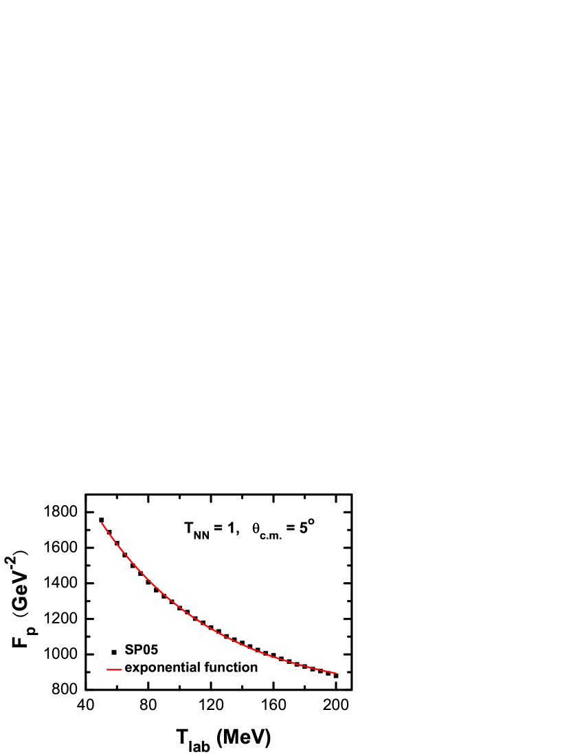
Figure 1: (Color online) The experimental SP05 pseudoscalar amplitudes $T_{NN}=1$ $F_{p}$, represented by the solid squares, as a function of the laboratory kinetic energy $T_{\rm{lab}}$ for a small centre-of-mass scattering angle of 5 degrees. The solid curve is an exponential function of the form given by Eq. (46).

A clear exponential energy-dependence is observed. Guided by the latter trend, we chose the following exponential energy-dependence for all (both real and imaginary) coupling constants, namely

$$g^{2}(E)\ =\ g^{2}_{0}[1\ +\ a_{g}(e^{a_{T}T_{\rm{rel}}}\ -\ 1)]$$ (46)

where

$$T_{\rm{rel}}\equiv\frac{T_{0}-T_{\rm{lab}}}{T_{0}}$$ (47)

with $T_{0}=200$ MeV, $T_{\rm{rel}}$ is positive in the 50 to 200 MeV energy range of interest, and $g^{2}_{0}$, $a_{g}$ and $a_{T}$ are dimensionless parameters extracted by fitting to the relevant data. For the real meson masses we chose the experimentally measured values Ha02 for the $\pi$, $\omega$ and $\rho$ mesons, namely 138, 782, and 770 MeV, respectively. For the other real and imaginary meson masses, as well as the real and imaginary cutoff energies $\Lambda_{i}$ and $\bar{\Lambda}_{i}$, we chose the starting the values to be the same as those published in Table I of Ref. Ma96 .

Firstly, the meson masses, coupling constants and cutoff parameters were varied slightly to obtain the best fit to the 200 MeV data alone. Similar to Ref. Ma96 , the values of $\Lambda_{i}$ and $\bar{\Lambda}_{i}$ were restricted to always exceed the respective meson masses. Thereafter, the meson masses and cutoff parameters were kept fixed, and $a_{g}$ and $a_{T}$, which determine the coupling constants via Eq. (46), were varied to obtain the best fit to the total data set between 50 and 200 MeV. Then all parameters (with the exception of the meson masses) were varied to fit the total data set.

IV Results

The fits to the real and imaginary amplitudes yield minimum $\chi^{2}$ values of 10.203 and 10.798, respectively: the relative $\chi^{2}$ values can be obtained by dividing the latter values by 2450. The fit to the real part of amplitude $a$ for $I_{NN}=0$ was found to be inferior compared to the real parts of the other amplitudes. Therefore, for the real part, the weight of amplitude $a$ was multiplied by 200, and the new $\chi^{2}$ value is equal to 16.657. The imaginary parts of amplitudes $b$, $c$ for $I_{NN}=1$ and $a$, $b$, $c$ for $I_{NN}=0$ showed systematic deviations in the low energy range. For the imaginary amplitudes, the parameter $a_{T}$ of the isovector tensor meson was changed slightly, such that the systematic deviation nearly disappeared, and the fits to the other amplitudes remained satisfactory. Fitted values for the various HLF parameters are presented in Table 2.

Table 2: Real and imaginary HLF parameters. The masses $m$ and cutoff parameters $\Lambda$ are in MeV, whereas the other parameters are dimensionless.

Real parameters
Meson	Isospin	Coupling type	m	$g^{2}_{0}$	$a_{g}$	$a_{T}$	$\Lambda$
$\sigma$	0	Scalar (S)	600	-8.379	$-5.581\times 10^{-1}$	$2.364\times 10^{-1}$	965.23
$\omega$	0	Vector (V)	782	$1.014\times 10^{1}$	$-2.219\times 10^{-2}$	3.793	1158.74
$t_{0}$	0	Tensor (T)	550	$2.783\times 10^{-1}$	1.331	3.074	1955.59
$a_{0}$	0	Axial vector (A)	500	$4.842\times 10^{-1}$	1.440	2.847	1577.53
$\eta$	0	Pseudoscalar (P)	950	$1.089\times 10^{1}$	1.553	1.956	980.99
$\delta$	1	Scalar (S)	500	$6.233\times 10^{-3}$	5.675	3.521	3000.00
$\rho$	1	Vector (V)	770	$-1.535\times 10^{-1}$	3.429	$1.825\times 10^{-1}$	3000.00
$t_{1}$	1	Tensor (T)	600	$-2.497\times 10^{-1}$	$5.508\times 10^{-1}$	3.959	1290.72
$a_{1}$	1	Axial vector (A)	650	-1.355	$2.480\times 10^{-1}$	3.623	745.19
$\pi$	1	Pseudoscalar (P)	138	$1.195\times 10^{1}$	$-1.671\times 10^{-1}$	$3.216\times 10^{-1}$	678.44
Imaginary parameters
Meson	Isospin	Coupling type	m	$\bar{g}^{2}_{0}$	$\bar{a}_{g}$	$\bar{a}_{T}$	$\bar{\Lambda}$
$\sigma$	0	Scalar (S)	600	-2.866	$7.722\times 10^{-1}$	1.503	772.74
$\omega$	0	Vector (V)	700	4.415	$7.094\times 10^{-1}$	1.528	701.00
$t_{0}$	0	Tensor (T)	750	$-9.114\times 10^{-1}$	1.217	1.674	1395.12
$a_{0}$	0	Axial vector (A)	750	-2.124	1.187	1.524	1364.90
$\eta$	0	Pseudoscalar (P)	1000	$1.411\times 10^{1}$	$3.021\times 10^{-2}$	4.970	3000.00
$\delta$	1	Scalar (S)	650	3.089	$9.873\times 10^{-1}$	$8.292\times 10^{-1}$	771.14
$\rho$	1	Vector (V)	600	-2.464	$7.620\times 10^{-1}$	1.176	795.81
$t_{1}$	1	Tensor (T)	750	$6.447\times 10^{-1}$	$3.316\times 10^{-1}$	2.977	1741.21
$a_{1}$	1	Axial vector (A)	1000	2.328	$3.885\times 10^{-1}$	2.915	1256.95
$\pi$	1	Pseudoscalar (P)	500	-5.788	$7.635\times 10^{-1}$	1.623	1391.26

To demonstrate the quality of the fits we compare, in Figs. (2) to (4), the fitted amplitudes $a$, $b$, $c$, $d$, and $e$, for both $T_{NN}=(0,1)$, to the corresponding SP05 empirical values at selected energies of 50, 125 and 200 MeV. Our HLF parameter set provides a satisfactory description of the empirical amplitudes at the latter energies. Although not displayed, this is also the case at all other energies between 50 and 200 MeV.

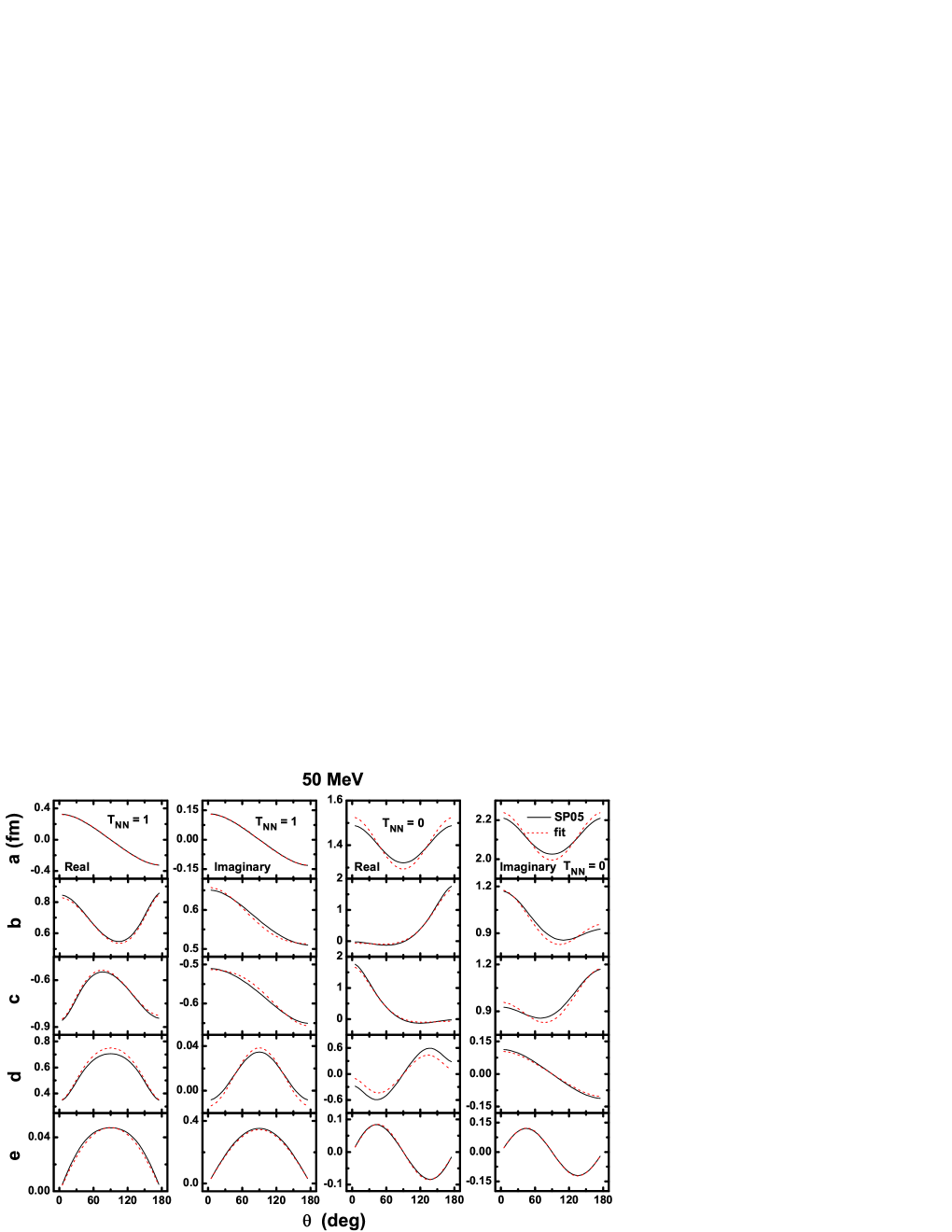
Figure 2: (Color online) Comparison of the fitted real and imaginary ($a,b,c,d,e$) $T_{NN}=1$ and $T_{NN}=0$ amplitudes (dashed curve), in units of fm, with the empirical SP05 amplitudes (solid curve) Arndt as a function of the NN centre-of-mass angle $\theta$, in degrees, at a laboratory kinetic energy 50 MeV.

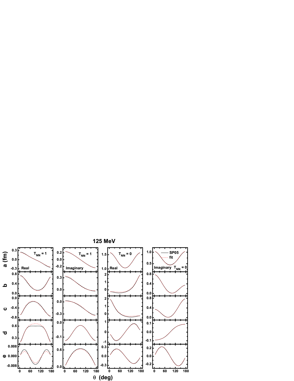
Figure 3: (Color online) Comparison of the fitted real and imaginary ($a,b,c,d,e$) $T_{NN}=1$ and $T_{NN}=0$ amplitudes (dashed curve), in units of fm, with the empirical SP05 amplitudes (solid curve) Arndt as a function of the NN centre-of-mass angle $\theta$, in degrees, at a laboratory kinetic energy 125 MeV.

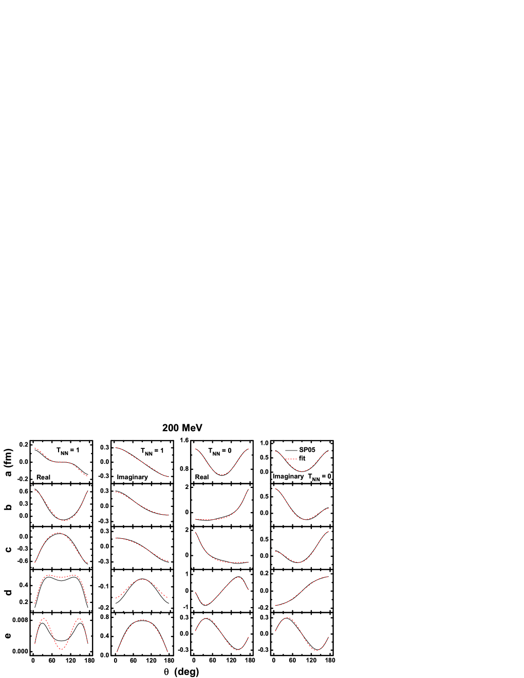
Figure 4: (Color online) Comparison of the fitted real and imaginary ($a,b,c,d,e$) $T_{NN}=1$ and $T_{NN}=0$ amplitudes (dashed curve), in units of fm, with the empirical SP05 amplitudes (solid curve) Arndt as a function of the NN centre-of-mass angle $\theta$, in degrees, at a laboratory kinetic energy 200 MeV.

The quality of our fit is also judged by comparing $pp$ and $pn$ HLF-based and empirical scattering observables derived from the $a,b,c,d,e$ amplitudes. In order to calculate the relevant $pp$ and $pn$ observables it is necessary to extract the corresponding $pp$ and $pn$ amplitudes via the following relation:

$$F_{i}(pp)\ =\ F_{i}(T=1)$$ (48)

$$F_{i}(pn)\ =\ \frac{1}{2}[F_{i}(T=1)\ +\ F_{i}(T=0)]\;,$$ (49)

and then convert them to $a,b,c,d,e$ amplitudes via Eq. (16). For eventual comparison to experimental observables, one must add Coulomb corrections (which dominate at forward and backward scattering angles) to the $a,b,c,d,e$ amplitudes for $T_{NN}=1$: the Coulomb amplitudes were obtained by subtracting the SAID $T_{NN}=1$ amplitudes from the SAID $pp$ amplitudes. The NN scattering observables of interest are defined as follows Ho85 :

$$\sigma = \frac{1}{2}(|a|^{2}+|b|^{2}+|c|^{2}+|d|^{2}+|e|^{2})$$

$${\rm{P}} = \text{Re}(a^{*}e)/\sigma$$

$${\rm{D}} = D_{nn}=\frac{1}{2}(|a|^{2}+|b|^{2}-|c|^{2}-|d|^{2}+|e|^{2})/\sigma$$

$${\rm{A}}_{yy} = \frac{1}{2}(|a|^{2}-|b|^{2}-|c|^{2}+|d|^{2}+|e|^{2})/\sigma$$

$${\rm{R}} = D_{s^{\prime}s}=\left[\text{Re}(a^{*}b)\cos(\alpha+\frac{\theta}{2})+\text{Re}(c^{*}d)\cos(\alpha-\frac{\theta}{2})-\text{Im}(b^{*}e)\sin(\alpha+\frac{\theta}{2})\right]/\sigma$$

$${\rm{A}} = {\rm{D}}_{s^{\prime}\ell}=\left[-\text{Re}(a^{*}b)\sin(\alpha+\frac{\theta}{2})+\text{Re}(c^{*}d)\sin(\alpha-\frac{\theta}{2})-\text{Im}(b^{*}e)\cos(\alpha+\frac{\theta}{2})\right]/\sigma$$

where

$$\alpha=\frac{\theta}{2}-\theta_{\rm{lab}}\;$$ (50)

with $\theta_{\rm{lab}}$ being the laboratory scattering angle, and $\sigma=d\sigma/d\Omega$ represents the unpolarized differential cross section.

Before comparing empirical NN scattering observables to our optimal HLF predictions, we briefly comment on the parameter-sensitivity of the latter. We have established that the lower energy observables are more sensitive to variations in the values of $g^{2}$ [calculated from $g_{0}^{2}$, $a_{g}$ and $a_{T}$ in Eq. (46)]. For example, for $pp$ scattering at 50 MeV, variations of 1 % in the $g^{2}$ values translate to a maximum change of 6 % on the polarization (${\rm{P}}$), the effect being reduced for all other spin observables, and also modify the unpolarized differential cross section ($d\sigma/d\Omega$) by 15 %, where the latter corresponds to a 1 % change in the real isoscalar tensor coupling. On the other hand, all the $pn$ observables exhibit less sensitivity.

Results for the unpolarized differential cross section ($d\sigma/d\Omega$), the polarization (${\rm{P}}$), the depolarization (${\rm{D}}$), the tensor asymmetry (${\rm{A}}_{yy}$)and triple scattering parameters ${\rm{A}}$ and ${\rm{R}}$ are shown in Fig. (5) to (7) for $pp$ and $pn$ at three different energies, namely 50, 125 and 200 MeV. In general, our HLF parameterization provides an excellent description of the empirical scattering observables. In particular, the quality of our fits is just as good,if not better, than those presented in Refs. Ho85 ; Ma96 ; Ma98 . Although this paper focussed on the 50 to 200 MeV range, we have also confirmed that our parametrization provides a satisfactory description of scattering observables at a lower enery limit of 40 MeV and a higher energy limit of 300 MeV. The next phase of this project will be to test the predictive power of the relativistic $t\rho$ folding procedure (for generating microscopic relativistic scalar and vector optical potentials) for describing elastic proton scattering from nuclei at energies lower than 200 MeV. Indeed, at these low energies, Pauli blocking corrections and nuclear medium modifications to the NN interaction will play a significant role Mu87 ; De00 ; De05 . RIA predictions as well as the importance of the latter corrections for elastic proton scattering will be presented in a forthcoming paper.

This work is partly supported by Major State Basic Research Developing Program 2007CB815000, the National Natural Science Foundation of China under Grant Nos. 10435010, 10775004 and 10221003, as well as the National Research Foundation of South Africa under Grant No. 2054166.

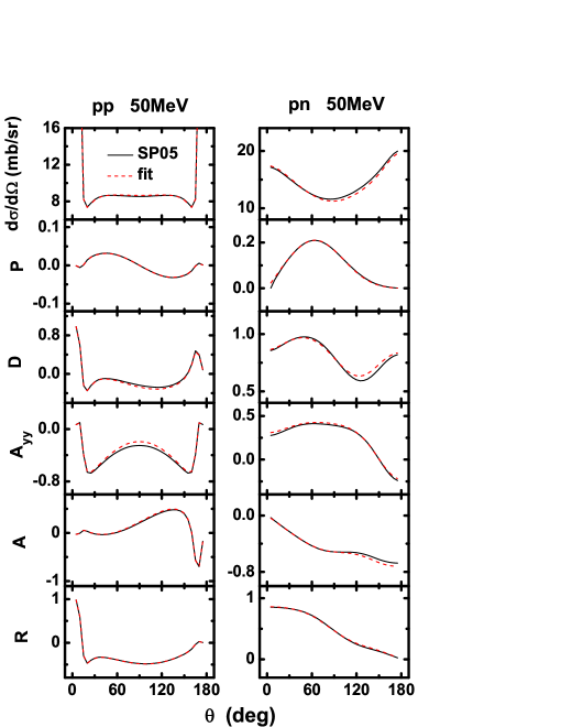
Figure 5: (Color online) $pp$ and $pn$ scattering observables versus the centre-of-mass angles $\theta$ at an incident laboratory kinetic energy of $T_{\rm{lab}}=50$ MeV.

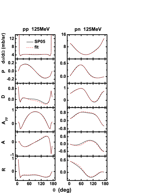
Figure 6: (Color online) $pp$ and $pn$ scattering observables versus the centre-of-mass angles $\theta$ at an incident laboratory kinetic energy of $T_{\rm{lab}}=125$ MeV.

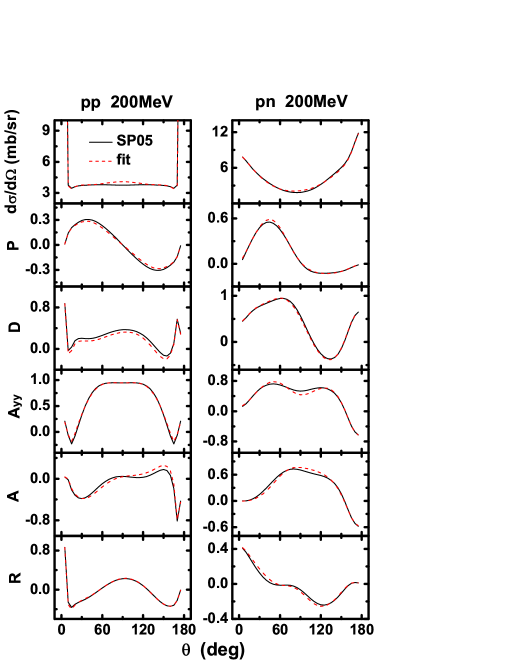
Figure 7: (Color online) $pp$ and $pn$ scattering observables versus the centre-of-mass angles $\theta$ at an incident laboratory kinetic energy of $T_{\rm{lab}}=200$ MeV.

References

- (1) C. J. Horowitz, Phys. Rev. C 31, 1340 (1985).
- (2) D. P. Murdock and C. J. Horowitz, Phys. Rev. C 35, 1442 (1987).
- (3) O. V. Maxwell, Nucl. Phys. A600, 509 (1996).
- (4) O. V. Maxwell, Nucl. Phys. A638, 747 (1998).
- (5) T. Noro, T. Yonemura, S. Asaji, N. S. Chant, K. Fujita, Y. Hagihara, K. Hatanaka, G. C. Hillhouse, T. Ishida, M. Itoh, S. Kishi, M. Nakamura, Y. Nagasue, H. Sakaguchi, Y. Sakemi, Y. Shimizu, H. Takeda, Y. Tamesige, S. Terashima, M. Uchida, T. Wakasa, Y. Yasuda, H. P. Yoshida, and M. Yosoi. Phys. Rev. C 72, 041602(R) (2005).
- (6) Junji Mano and Yoshiteru Kudo. Prog. Theor. Phys. 100, 91 (1998).
- (7) F. Hofmann, C. Bäumer, A. M. van den Berg, D. Frekers, V. M. Hannen, M. N. Harakeh, M. A. de Huu, Y. Kalmykov, P. von Neumann-Cosel, V. Yu. Ponomarev, S. Rakers, B. Reitz, A. Richter, A. Shevchenko, K. Schweda, J. Wambach and H. J. Wörtche. Phys. Lett. 612B, 165 (2005).
- (8) E. D. Cooper, S. Hama, B. C. Clark and R. L. Mercer. Phys. Rev. C 47, 297 (1993).
- (9) J. Meng, H. Toki, S. G. Zhou, S. Q. Zhang, W. H. Long and L. S. Geng. Prog. Part. Nucl. Phys. 57, 470 (2006).
- (10) B. G. Todd and J. Piekarewicz, Phys. Rev. C 67, 044317 (2003).
- (11) P. K. Deb and K. Amos, Phys. Rev. C 62, 024605 (2000).
- (12) P. K. Deb, B. C. Clark, S. Hama, K. Amos, S. Karataglidis and E. D. Cooper, Phys. Rev. C 72, 014608 (2005).
- (13) J. Bystricky, F. Lehar, and P. Winternitz, Le Journal de Physique39, 1 (1978).
- (14) J. A. McNeil, L. Ray, and S. J. Wallace, Phys. Rev. C 27, 2123 (1983).
- (15) M. Fierz, Z. Phys. 104, 533 (1937).
- (16) K. Hagiwara, et al. (Particle Data Group), Phys. Rev. D 66, 010001(2002).
- (17) R. A. Arndt and D. Roper, VPI and SU Scattering Analysis Interactive Dial-in Program and Data Base (SAID).