Spectral weight transfer in a disorder-broadened Landau level

In the absence of disorder, the degeneracy of a Landau level (LL) is $N=BA/\phi_{0}$, where $B$ is the magnetic field, $A$ is the area of the sample and $\phi_{0}=h/e$ is the magnetic flux quantum. With disorder, localized states appear at the top and bottom of the broadened LL, while states in the center of the LL (the critical region) remain delocalized. This well-known phenomenology is sufficient to explain most aspects of the Integer Quantum Hall Effect (IQHE) Klitzing80 . One unnoticed issue is where the new states appear as the magnetic field is increased. Here we demonstrate that they appear predominantly inside the critical region. This leads to a certain “spectral ordering” of the localized states that explains the stripes observed in measurements of the local inverse compressibility Ilani04 ; Martin04 , of two-terminal conductance Cobden99 , and of Hall and longitudinal resistances Jouault07 without invoking interactions as done in previous work Pereira06 ; Struck06 ; Sohrmann06 .

The spectrum and eigenstates of a disorder-broadened LL can be studied with the well-established approach of diagonalizing the single electron Hamiltonian

$${\cal H}={(2m_{e})^{-1}}\left[-i\hbar\nabla+e{\bf A}({{\bf r}})\right]^{2}+V({\bf r}),$$ (1)

where we choose ${\bf A}({{\bf r}})=(0,Bx)$, $V({\bf r})$ is the disorder, and periodic boundary conditions (PBC) are applied to a system of area $A=L\times L$. Properties of single particle states, such as the localization length, are calculated for each eigenstate and then averaged over disorder realizations. Many-body wavefunctions (Slater determinants) are constructed from these single-electron states. Usually, in theoretical studies the magnetic field is kept fixed at a value $B=N\phi_{0}/L^{2}$, where $N$ is an integer defining the dimension of the LL subspace, and one sweeps the electron density $n_{e}$ or, equivalently, the filling factor $\nu=n_{e}A/N$, by adjusting the Fermi energy $E_{F}$.

Since the experiments mentioned above investigate behavior of various quantities in the $(n_{e},B)$ plane, we need to understand how the spectrum changes when $B$ is also tuned. Given the constraint that an integer number of fluxes must penetrate the sample, $B$ can only change in discrete steps of $\phi_{0}/L^{2}$. Therefore, we ask the following question: How do single electronic wavefunctions evolve when one more magnetic flux is inserted?

Let $|i,N\rangle$, $1\leq i\leq N$ be the eigenstates of a spin-polarized LL corresponding to a given disorder $V({\bf r})$ and a magnetic field $B=N\phi_{0}/L^{2}$. The states are ordered by their energies $E_{1}<E_{2}<...<E_{N}$ (accidental degeneracies can be lifted with minute changes in $V({\bf r})$).

To see how the wavefunctions evolve when $B$ increases, we calculate their disorder-averaged overlaps:

$$\overline{D}_{N}(i,j)=\overline{\left|\left<i,N|j,N+1\right>\right|^{2}},$$ (2)

where $1\leq i\leq N$ and $1\leq j\leq N+1$ label two eigenstates of the Hamiltonian (1) with the same disorder potential but different magnetic fields. The overline indicates a disorder average. In the results presented here we typically average over 1000 disorder realizations, and show results only for the spin-polarized lowest LL. Similar results are expected in higher LLs. The disorder potential $V({\bf r})$ is modeled as a sum of many short range, randomly placed Gaussian scatterers. We show 4 sets of data, for $L=50,128,200,750$ nm, $N=50,128,200,550$ and therefore $B=1.654$ T for the first three data sets, and 2.022 T for the last data set.

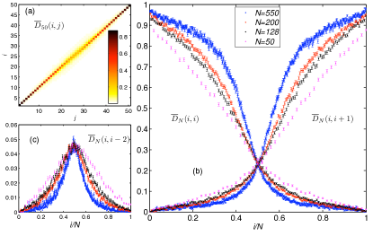
Figure 1: Overlap between eigenstates with an additional magnetic flux quantum. (a) Plot of the 50 by 51 overlap matrix $\overline{D}_{50}$, defined in Eq. (2). Only elements near the diagonal are visible. (b) $\overline{D}_{N}(i,i)$ and $\overline{D}_{N}(i,i+1)$ vs. filling factor $i/N$ for 4 different sizes $N=50,128,200,550$. The transition region narrows towards half filling as $N$ increases. (c) Typical off-diagonal overlap matrix elements $\overline{D}_{N}(i,i-2)$ vs. $i/N$, for the same values of $N$. These are much smaller than the main diagonal elements shown in (b). The peak narrows as $N$ increases.

The $N$ by $N+1$ matrix $\overline{D}_{N}(i,j)$ is almost zero everywhere except near its diagonal, as shown in Fig. 1(a). Focusing on this region in Fig 1(b), we see that $\overline{D}_{N}(i,i)$ decreases from near unity to near zero as $i$ increases from 1 to $N$, while $\overline{D}_{N}(i,i+1)$ is almost the mirror image of $\overline{D}_{N}(i,i)$. They intersect at $j/N\approx 1/2$, i.e. half filling, where they seem to have a universal value, which is independent of $N$ and $B$. These elements change most rapidly in a region near half-filling, which becomes narrower as $N$ increases. Other matrix elements, e.g. $\overline{D}_{N}(i,i-2)$ shown in Fig. 1(c), exhibit a very small peak in this narrow region which we identify as the critical region.

Since the overlap of Eq. (2) measures the similarity of eigenstates, these results show that the new state created when $B$ increases by one flux quantum appears predominantly in the center of the disorder-broadened LL. Localized states at the bottom of the LL are little affected and keep the same spectral ordering leading to large $\overline{D}_{N}(i,i)$ overlaps. Localized states at the top of the LL also keep their spectral ordering but shifted upward by 1, to account for the new eigenstate created in the critical region. This explains why $\overline{D}_{N}(i,i+1)$ is here close to unity.

The appearance of the new state amongst the delocalized states is not surprising since such states can enclose a large area, with sufficient of the additional magnetic flux going through, and therefore the effects of the small $\delta B=\phi_{0}/L^{2}$ increase are not perturbative even for a large $B$. By contrast, for localized states the effect of the additional flux is perturbatively small, leading only to slight spatial deformations of the wavefunctions.

This conclusion can also be reached using well-known results for the Hofstadter butterfly. To map into these, we use copies of the $L\times L$ system to tile the infinite plane, so that the disorder $V({\bf r})$ becomes periodic with period $L$. The resulting Hofstadter problem has as magnetic unit cell the $L\times L$ area, thus it corresponds to $BL^{2}/\phi_{0}=q/p=N$. The eigenstates of Hamiltonian (1) are now magnetic Bloch waves $\psi_{i,\bf k}({\bf r})=e^{-i{\bf k}\cdot{\bf r}}u_{i,{\bf k}}({\bf r})$. The integer $i$ labels the $q=N$ magnetic Bloch bands (MBBs) originated from an LL. The functions $u_{i,{\bf k}}({\bf r})$ satisfy generalized PBC Thouless82 . In effect, each of the $N$ eigenstates of an LL of the finite-size $L\times L$ system has evolved into an MBB of the Hofstadter problem (the former are the ${{\bf k}}=0$ states of the latter). As a result, we can associate to each eigenstate of the finite-size system the Chern number $\sigma_{i}$ of the corresponding MBB Thouless82 . $\sigma_{i}$ is well defined for each MBB, because energy bands $E_{i}({\bf k})$ and $E_{i+1}({\bf k})$ can only touch at discrete ${\bf k}$ points, and small changes in $V({{\bf r}})$ can remove such degeneracies, as implicitly assumed when $\sigma_{i}$ is calculated in Refs. Huo92 ; Yang97 .

Thouless showed that localized states have zero Chern numbers Thouless84 . This is easy to understand, since localized states are rather insensitive to changes in the boundary conditions used to calculate the Chern number Thouless82 . This is verified by numerical calculations and finite size scaling analysis Huo92 ; Yang97 showing that the non-zero Chern numbers are distributed near the center of the LL. The distribution fits the scaling theory of IQHE Pruisken87 ; Huckestein90 with the correct localization exponent $\nu=2.34\pm 0.04$ Huckestein90 ; Wei88 .

When the magnetic field is increased by $\phi_{0}/L^{2}$, i.e. $N\rightarrow N+1$, a new MBB must appear in the spectrum generated from each LL, thus one of the original MBBs must split into two. We now argue that only an MBB with a non-zero Chern number can do this, in other words the new MBB (new state) appears in the critical region.

A simple proof is obtained from combining Thouless et al.’s famous proportionality between the conductance of a MBB and its Chern number Thouless82 , and Středa’s formula Streda linking the conductance to the change in the density of states with changing $B$. This gives an expression for the Chern number:

$$\sigma_{i}=he^{-1}{\partial N_{i}(B)/\partial B},$$ (3)

where $N_{i}(B)$ is the density of states in the $i$th MBB. If this corresponds to a localized state, then $\sigma_{i}=0$ Thouless84 and this MBB cannot be the origin of the new state since its density of states stays unchanged as $B$ varies. The new electronic state in this LL must therefore originate from subbands having non-zero Chern numbers.

Another proof for the above result is obtained from the semi-classical theory of Chang and Niu Niu95 ; Niu85 . If $\delta B=\phi_{0}/L^{2}$ supplies the additional flux quantum, the quantization condition of hyperorbits in the MBB reads

$${\hbar\over 2e\delta B}\oint_{C_{m}}({\bf k}\times d{\bf k})\cdot{\bf z}+\Gamma_{i}(C_{m})=2\pi(m+1/2),$$ (4)

where $m$ is an integer and $\Gamma_{i}(C_{m})$ is the contour integral over an effective gauge field ${\cal A}_{i}$. Chang and Niu obtained the entire hierarchical structure of the Hofstadter butterfly by approximating the integral in Eq. (4) with the area of the magnetic Brillouin zone, and replacing $\Gamma_{i}(C_{m})$ with the Chern number. If $\sigma_{i}=0$, the localized wavefunction $\psi_{i}({\bf k})$ can be expanded as an absolutely convergent sum of Wannier functions Thouless84 , and the curvature of ${\cal A}_{i}$ vanishes identically. Thus, $\Gamma_{i}(C_{m})$ indeed vanishes for any localized MBB regardless of the shape of the hyperorbit $C_{m}$. Also, since our magnetic Brillouin zone is $[-\pi/L,\pi/L)\times[-\pi/L,\pi/L)$ by construction, the l.h.s. of Eq. (4) is found to be less or equal to $\pi$. It follows that $m=0$ is the unique possibility for the MBB of a localized state, i.e. such an MBB does not split into multiple MBBs when the magnetic field increases by $\delta B$ Niu95 ; Niu85 . Note that both these arguments are only valid if gaps between neighboring MBBs remain open as $B$ increases by $\delta B$. As already argued, this is expected to be typically the case, since accidental degeneracies closing the gap can be removed by small changes in the disorder $V(\bf r)$.

A nice illustration of this property is given by the very simple “disorder” potential $V({\bf r})\sim\cos(2\pi x/L)+\cos(2\pi y/L)$. Of course, this leads to the well-known Hofstadter butterfly spectrum, whose lower half is shown in Fig. 2. In accordance with our discussion, we are only interested in magnetic fields $B$ corresponding to $q/p=N$, for large $N$, marked by thick lines in the figure. As expected, there are $N$ MBBs (for even $N$, the two central MBBs just touch). When $N\rightarrow N+1$, a new MBB is spawned from the central MBB(s), which is the only one with a non-zero Chern number. Indeed, if $N$ is odd, the central subband evolves into two subbands, whereas if $N$ is even, a new subband grows out in the center. The outside MBBs have zero Chern numbers, and indeed correspond to states localized about the bottom/top of this “disorder” potential. As argued above, the spectrum of a general disorder potential also has these properties, except that typically there are several MBBs with non-zero Chern numbers, one of which will generate the new state when $B$ increases by one magnetic flux.

To summarize, all these numerical and theoretical arguments prove that the new states generated in a disorder-broadened LL when the magnetic field increases appear predominantly in the critical region. After a state is expelled to the upper (lower) localized regions as $B$ increases, its order from the top (bottom) of the LL remains essentially fixed.

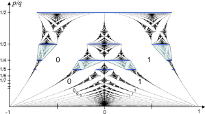
Figure 2: Lower half of a Hofstadter butterfly. The subbands for $p=1,q=N$ are marked by thick blue lines. The Hall conductances in units of $e^{2}/h$ are given for the main gaps, which never close as $B\sim q/p$ increases. The shaded blocks are typical self-similar spectra generated by an MBB when an additional flux is inserted ($N\rightarrow N+1$). The new spectral weight as $B$ increases always appears in the center of the LL.

This spectral ordering is the main ingredient needed for understanding the results of recent single-electron transistor (SET) measurements Yoo97 ; Zhitenev00 that investigate the charge distribution of localized electronic states in two-dimensional electron systems Ilani04 ; Martin04 , as well as of measurements of mesoscopic fluctuations of two-terminal conductances Cobden99 and of Hall and longitudinal resistances Jouault07 . When plotted in the $(n_{e},B)$ plane, the maxima in these quantities are found to track straight lines with certain quantized values for their slopes, as described below. This suggests that such “stripes” are an intrinsic aspect of IQHE phenomenology. In fact, SET and transport experiments are strikingly complementary to each other. When their results are put together, as schematically shown in Fig. 3, we get a complete picture of these stripes: States belonging to the $n$th LL are located between the straight lines $n_{e}=nB/\phi_{0}$ and $n_{e}=(n+1)B/\phi_{0}$. In the upper half of this LL, stripes are found to be parallel with $n_{e}=(n+1)B/\phi_{0}$, while in the lower half, stripes are parallel to $n_{e}=nB/\phi_{0}$. Near the center of the LL, stripes of both slopes are visible and can cross each other. Ref. Ilani04 images the stripes close to the LL edges, while Refs. Cobden99 ; Jouault07 image the stripes near LL centers.

So far it has been unanimously agreed that these stripes are signatures of Coulomb-blockade physics in the localized states Pereira06 ; Struck06 ; Sohrmann06 . We now argue that the main reason for these stripes’ appearance is in fact the spectral ordering discussed above, which is a single-electron effect. Interactions do play a role through screening, as discussed below, but it is very much a secondary one.

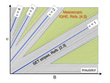
Figure 3: A schematic composite picture (computer-generated) of the stripes observed experimentally in Refs. Ilani04 ; Martin04 ; Cobden99 ; Jouault07 .

We begin our discussion with the SET results that measure the “local inverse compressibility” $d\mu/dn_{e}$, which is a local DC response function dominated by localized states located under the SET tip. Consider the evolution of a maximum due to one such localized state, for example one that is found near the bottom of the $n$th LL. If the magnetic field is increased by $\delta B=\phi_{0}/L^{2}$, $n$ new states appear near the centers of the lower $n$ LLs (counting from $n=0$). As a result, in order to bring the Fermi level back to this particular state so as to see the same maximum, $n_{e}$ must be increased by $\delta n_{e}=n/L^{2}$. Thus, the maximum moves along a line of slope $\delta n_{e}/\delta B=n/\phi_{0}$. For a state at the top of the $n$th LL, however, the density change must be $\delta n_{e}=(n+1)/L^{2}$, since the spectral position of this state is also shifted upwards by the new state appearing near the center of the $n$th LL itself. Thus, maxima due to these states will have a slope of $(n+1)/\phi_{0}$, precisely as seen in experiments.

It is worth noting that Fig 4. of Ref. Sohrmann06 shows that even if the Coulomb interaction is turned off, stripes do appear with essentially the right slopes. The authors argue that these are not in agreement with experiment because the region occupied by them increases with $B$, whereas in experiments one sees a roughly constant number of maxima, as sketched in Fig. 3. Addition of Coulomb interactions fixes this problem, but this is because of screening: their results show that the stronger the interaction, the more effective the screening, the fewer states (maxima) are seen. We therefore argue that Coulomb interactions (screening) have the secondary role of limiting the number of localized states “visible” to the tip, but the stripes’ slopes are determined purely by single-electron physics.

Note that this explanation relies essentially on the fact that localized states tend to keep their spectral order with respect to the top or bottom of the LL. Of course, states localized about the same minimum or maximum in the disorder landscape do keep their relative spectral ordering, but it is possible that the energies of states localized in different spatial regions might cross each other as $B$ varies. Such events must be rare, as our simulations in Fig. 1 show; in fact, we find that $\overline{D}_{N}(i,i)$ and $\overline{D}_{N}(i,i+1)$ get closer to 1 in the relevant interval when $N$ increases! However, if such a rare crossing does take place for one of the states under the SET tip, the maximum will shift by $\delta n_{e}=\pm 1/L^{2}$ at the $B$ value where the crossing occurs, after which the stripe resumes with the correct slope. Such jumps would be rather impossible to measure.

The stripes in the transport measurements have the same origin. Here, the mesoscopic fluctuations are caused by electronic states that mediate the charge transport across the Hall bar, as shown in Ref. Zhou05 ; Berciu05 . For example, the fluctuations in the two-terminal conductance measured in Ref. Cobden99 are due to Jain-Kivelson tunneling Jain88 through electronic states located in the central region of the sample. To see the same resonance, the Fermi level must be tuned to match the energy of the state mediating the tunneling, so one expects to see the maxima following lines of quantized slopes in the $(n_{e},B)$ plane for the same reasons given above. However, unlike for SET measurements, the Fermi level is now near the center of the LL, where the transition between quantum Hall plateaus occurs. When an additional $\phi_{0}$ is inserted, there may be either $n$ or $n+1$ new states below the Fermi level. As a result, one expects to see stripes with both slopes. Occasional crossings of stripes is also expected, when the states mediating their tunneling are more than a coherence length $L_{\phi}$ apart, i.e. there is no quantum interference between these two tunneling events.

These arguments also explain the stripes observed in SET measurements  Martin04 in the fractional quantum Hall effect (FQHE) Tsui82 . It is well known that FQHE can be explained as IQHE of quasi-particles Laughlin83 ; Haldane83 ; Jain89 . Our explanation of the stripes in the IQHE regime is equally applicable to the FQHE regime, except with electrons replaced by these quasi-particles.

In conclusion, we claim that the spectral ordering of states within a LL, demonstrated in the first part of this work, is the main ingredient needed to understand the stripes observed in SET and transport measurements. Unlike other authors who identify them as effects of interactions, we find that single-electron physics suffices to explain, in a unified manner, all these observations. This is gratifying, given the long-standing success of the non-interacting electron approximation in describing all other aspects of IQHE physics.

- (1) v. Klitzing, K., Dorda, G., & Pepper, M. New Method for High-Accuracy Determination of the Fine-Structure Constant Based on Quantized Hall Resistance. Phys. Rev. Lett. 45, 494-497 (1980).
- (2) Ilani, S., et al. The microscopic nature of localization in the quantum Hall effect. Nature 427, 328-332 (2004).
- (3) Martin, J. et al. Localization of Fractionally Charged Quasi-Particles. Science 305, 980-983 (2004).
- (4) Cobden, D. H., Barnes, C. H. W. & Ford, C. J. B. Fluctuations and Evidence for Charging in the Quantum Hall Effect. Phys. Rev. Lett. 82, 4695-4698 (1999).
- (5) Jouault, B. private communication.
- (6) Pereira, A. L. C. & Chalker, J. T. Electrostatic theory for imaging experiments on local charges in quantum Hall systems. Physica E 31, 155-159 (2006).
- (7) Struck A. & Kramer, B. Electron Correlations and Single-Particle Physics in the Integer Quantum Hall Effect. Phys. Rev. Lett. 97, 106801 (2006).
- (8) Sohrmann, C. & Römer, R. A.Compressibility stripes for mesoscopic quantum Hall samples New J. Phys. 9, 97-122 (2007).
- (9) Thouless, D. J. et al.. Quantized Hall Conductance in a Two-Dimensional Periodic Potential. Phys. Rev. Lett. 49, 405 (1982).
- (10) Huo, Y. & Bhatt, R.N. Current carrying states in the lowest Landau level. Phys. Rev. Lett. 68, 1375 (1992).
- (11) Yang, K.& Bhatt, R.N. Current-carrying states in a random magnetic field Phys. Rev. B 55, R1922 (1997).
- (12) Thouless, D. J., Wannier functions for magnetic sub-bands. J. Phys. C: Solid State Phys., 17, L325-L327 (1984).
- (13) Pruisken, A. M. M. Universal Singularities in the Integral Quantum Hall Effect.Phys. Rev. Lett. 61, 1297 (1988).
- (14) Huckestein, B. Scaling theory of the integer quantum Hall effect. Rev. Mod. Phys. 67, 357 (1995).
- (15) Wei, H. P., et al. Experiments on Delocalization and University in the Integral Quantum Hall Effect. Phys. Rev. Lett. 61, 1294 (1988).
- (16) Středa, P. Theory of quantised Hall conductivity in two dimensions. J. Phys. C: Solid State Phys. 15, L717-L721 (1982).
- (17) Chang, M.-C. & Niu, Q. Berry Phase, Hyperorbits, and the Hofstadter Spectrum. Phys. Rev. Lett. 75, 1348 (1995).
- (18) Chang, M.-C. & Niu, Q. Berry phase, hyperorbits, and the Hofstadter spectrum: Semiclassical dynamics in magnetic Bloch bands. Phys. Rev. B 53, 7010 (1985).
- (19) Yoo, M. J. et al. Scanning Single-Electron Transistor Microscopy: Imaging Individual Charges. Science 276, 579-582 (1997).
- (20) Zhitenev, N. B. et al., Imaging of localized electronic states in the quantum Hall regime. Nature 404, 473-476 (2000).
- (21) Zhou, C. & Berciu, M. Resistance fluctuations near integer quantum Hall transitions in mesoscopic samples. Europhys. Lett. 69, 602 (2005).
- (22) Zhou, C. & Berciu, M. Correlated mesoscopic fluctuations in integer quantum Hall transitions. Phys. Rev. B 72, 085306 (2005).
- (23) Jain, J. K. & Kivelson, S. A. Quantum Hall effect in quasi one-dimensional systems: Resistance fluctuations and breakdown. Phys. Rev. Lett. 60, 1542 (1988).
- (24) Tsui, D. C., Stormer, H. L. &Gossard, A. C. Two-Dimensional Magnetotransport in the Extreme Quantum Limit. Phys. Rev. Lett. 48, 1559 (1982).
- (25) Laughlin, R. B. Anomalous Quantum Hall Effect: An Incompressible Quantum Fluid with Fractionally Charged Excitations. Phys. Rev. Lett. 50, 1395 (1983).
- (26) Haldane, F. D. M. Fractional Quantization of the Hall Effect: A Hierarchy of Incompressible Quantum Fluid States. Phys. Rev. Lett. 51, 605 (1983).
- (27) Jain, J. K. Composite-fermion approach for the fractional quantum Hall effect. Phys. Rev. Lett. 63, 199 (1989).