Dependency and false discovery rate: Asymptotics

Abstract

Some effort has been undertaken over the last decade to provide conditions for the control of the false discovery rate by the linear step-up procedure (LSU) for testing $n$ hypotheses when test statistics are dependent. In this paper we investigate the expected error rate (EER) and the false discovery rate (FDR) in some extreme parameter configurations when $n$ tends to infinity for test statistics being exchangeable under null hypotheses. All results are derived in terms of $p$-values. In a general setup we present a series of results concerning the interrelation of Simes’ rejection curve and the (limiting) empirical distribution function of the $p$-values. Main objects under investigation are largest (limiting) crossing points between these functions, which play a key role in deriving explicit formulas for EER and FDR. As specific examples we investigate equi-correlated normal and $t$-variables in more detail and compute the limiting EER and FDR theoretically and numerically. A surprising limit behavior occurs if these models tend to independence.

Dependency and false discovery rate: Asymptotics AASupported by the Deutsche Forschungsgemeinschaft.

, and

1 Introduction

Control of the false discovery rate (FDR) in multiple hypotheses testing has become an attractive approach especially if a large number of hypotheses is at hand. The first FDR controlling procedure, a linear step-up procedure (LSU), was originally designed for independent $p$-values (cf. r1 ) and has its origins in r3 (cf. also r15 ). Meanwhile, it is known that the LSU-procedure controls the FDR even if the test statistics obey some special dependence structure. Key words are MTP₂ (multivariate total positivity of order 2) and PRDS (positive regression dependency on subsets). More formal descriptions of these conditions and proofs can be found in r2  and r14 . In view of testing problems with some ten thousand hypotheses as they appear, for example, in genetics, asymptotic considerations become more and more popular. The first asymptotic investigations concerning expected type I errors of the LSU-procedure, as well as for the corresponding linear step-down (LSD) procedure for the independent case, can be found in r9  and r10 . A first theoretical comparison of classical stepwise procedures controlling a multiple level $\alpha$ [or familywise error rate (FWER) in the strong sense] based on asymptotics is given in r5 . Moreover, attempts to improve the LSU-procedure and interesting investigations based on asymptotics can be found, for example, in r12 , r11 and r22 .

The LSU-procedure is based on the critical values $\alpha_{i:n}=i\alpha/n$, $i=1,\ldots,n$, introduced in r17 in a different context. Based on ordered $p$-values$p_{1:n}\leq\cdots\leq p_{n:n}$, the LSU-procedure rejects the corresponding hypotheses $H_{1:n},\ldots,H_{m:n}$, where $m=\max\{i\dvtx p_{i:n}\leq\alpha_{i:n}\}$. The corresponding LSD-procedure rejects $H_{1:n},\ldots,H_{r:n}$, where $r=\max\{i\dvtx p_{j:n}\leq\alpha_{j:n}\mbox{ for all }j=1,\ldots,i\}$. Since $m\geq r$, the LSU-procedure may reject more hypotheses than the LSD-procedure, never less. In this paper we restrict attention to the LSU-procedure, which can be rewritten in terms of the empirical c.d.f. (e.c.d.f.) ${F}_{n}$ (say) of the $p_{i}$’s. Setting $t^{*}=\sup\{t\dvtx{F}_{n}(t)\geq t/\alpha\}$, $H_{i}$ is rejected iff $p_{i}\leq t^{*}$. The rejection curve $r_{\alpha}(t)=t/\alpha$ will be called the Simes-line. Note that $\alpha_{i:n}=r_{\alpha}^{-1}(i/n)$. The threshold $t^{*}$ will be called the largest crossing point (LCP) between the e.c.d.f. and the Simes-line and plays a crucial role in this paper.

FDR control for a multiple test procedure is defined as follows. Let $V_{n}$ denote the number of falsely rejected null hypotheses and let $R_{n}$ denote the number of all rejections. Then the FDR (depending on the underlying parameter configuration $\vartheta\in\Theta$, say) is defined by

$$\operatorname{FDR}_{n}(\vartheta)=\mathbb{E}\biggl{[}\frac{V_{n}}{R_{n}\vee 1}\biggr{]}$$

and is said to be controlled at level $\alpha$ if

$$\sup_{\vartheta\in\Theta}\operatorname{FDR}_{n}(\vartheta)\leq\alpha.$$

The ratio $V_{n}/[R_{n}\vee 1]$ is the false discovery proportion (FDP). In the case of independent $p$-values both LSU and LSD control the FDR at level $\alpha$; more precisely, if $\vartheta\in\Theta$ is such that exactly $n_{0}$ hypotheses are true and the remaining $n_{1}=n-n_{0}$ ones are false, for both LSU and LSD, the actual FDR is bounded by $n_{0}\alpha/n$. Under weak additional assumptions, we have in this setting for the LSU-procedure

$$\operatorname{FDR}_{n}(\vartheta)=\frac{n_{0}}{n}\alpha.$$

Different proofs for this fact can be found in r1 , r9 , r14 and r22 .

In r10 the expected number of type I errors (ENE), that is, $\mathrm{ENE}_{n}(\vartheta)=\mathbb{E}[V_{n}]$, of LSU and LSD was investigated for the case that all hypotheses are true and $p$-values are independent. In this case the limiting ENE for $n\to\infty$ equals $\alpha/(1-\alpha)^{2}$ for LSU and $\alpha/(1-\alpha)$ for LSD. Moreover, in r9 the expected type I error rate (EER) defined by $\operatorname{EER}_{n}(\zeta)=\mathbb{E}[V_{n}/n]$ was studied if a proportion $1-\zeta$ of hypotheses is totally false, that is, with $p$-values equal to zero with probability $1$. For independent $p$-values, it was shown in r9 under quite general assumptions that for both LSU and LSD

$$\lim_{n\to\infty}\sup_{\vartheta\in\Theta}\mathbb{E}\biggl{[}\frac{V_{n}}{n}\biggr{]}=\bigl{(}1-\sqrt{1-\alpha}\bigr{)}^{2}/\alpha=\alpha/4+\alpha^{2}/8+O(\alpha^{3})\approx\alpha/4.$$

The worst case for the EER appears if the proportion of true hypotheses tends to $\zeta=(1-\sqrt{1-\alpha})/\alpha=1/2+\alpha/8+O(\alpha^{2})$, and, for small values of $\alpha$, the expected type I error rate is then approximately $\alpha/4$.

In this paper we investigate the behavior of EER and FDR of the LSU-procedure based on dependent test statistics if the number of hypotheses tends to infinity. It will be assumed that test statistics are exchangeable under the corresponding null hypotheses. The main issue will be the calculation of the limiting values of the actual EER and FDR in some extreme parameter configurations, where a proportion $\zeta_{n}$ of hypotheses will be assumed to be true and the remaining hypotheses will be assumed to be totally false. These configurations are least favorable for the EER, that is, EER becomes largest under these configurations if $\zeta_{n}$ is given. Theoretical results on least/most favorable configurations for the FDR (configurations where the FDR becomes largest/smallest) under dependence remain a challenging open problem. However, simulations indicate that extreme configurations ($n_{0}$ hypotheses true, $n_{1}$ hypotheses totally false) are first candidates for least favorable configurations and therefore of special theoretical interest. Until now, not many results are available concerning the behavior of EER and FDR under dependence. A brief discussion on expected type I errors for single-step procedures based on exchangeable test statistics and range statistics can be found in r8 .

In Section 2 we develop a general theory for the computation of the limiting EER and FDR assuming that exchangeable test statistics of the type $T_{i}=g(X_{i},Z)$ are at hand. The results heavily depend on the limit behavior of the e.c.d.f. of the underlying $p$-values given the value $z$ of the disturbance variable $Z$. Generally, the limiting e.c.d.f. $F_{\infty}$ (say) of dependent $p$-values differs substantially from that of independent $p$-values. Formulas for the limiting e.c.d.f. and crossing point determination are summarized in Lemma 2.1. For $\zeta_{n}\to\zeta\not=1$, limiting $\operatorname{EER}$ and $\operatorname{FDR}$ are computed in Theorems 1 and 3 in terms of the set of largest crossing points (LCP’s) between $F_{\infty}$ and the Simes-line. The case $\zeta_{n}\to 1$ is more complex because limiting LCP’s can be zero. For the latter case, we derive some important technical results for the FDR in Lemmas 4 and 5 supposing that the c.d.f. of a proportion of $p$-values is linear in a neighborhood of zero. The limiting $\operatorname{EER}$ and $\operatorname{FDR}$ are then computed in Theorems 6 and 8. Moreover, we give an example where the FDR is exactly the same as in the independent case. By utilizing the results of Section 2, we investigate equi-correlated normal variables in Section 3 and jointly studentized $t$-statistics in Section 4. The corresponding formulas for the limiting $\operatorname{EER}$ and $\operatorname{FDR}$ are given in Theorems 9 and 10 and Theorems 13 and 14, respectively. A surprising behavior of the FDR occurs if these models tend to independence and the proportion of false hypotheses tends to $0$; see Theorem 12 and Theorem 16. Some figures in Sections 3 and 4 illustrate the limiting behavior of EER and FDR. The numerical and computational effort for these graphs was enormous. A few concluding remarks are given in Section 5. Short proofs are in the main text, while more technical proofs are deferred to the Appendix.

2 Exchangeable test statistics: general considerations

We first consider the following basic model with exchangeable test statistics. Let $X_{i},\;i=1,\ldots,n$, be real-valued independent random variables with support $\mathcal{X}$. Moreover, let $Z$ be a further real-valued random variable, independent of the $X_{i}$’s, with support $\mathcal{Z}$ and continuous c.d.f. $W_{Z}$. Denote the c.d.f. of $X_{i}$ by $W_{i}$. Suppose the c.d.f. $W_{i}$ depends on a parameter $\vartheta_{i}\in[\vartheta_{0},\infty)$, where $\vartheta_{0}$ is known. Without loss of generality, it will be assumed that $\vartheta_{0}=0$. Consider the multiple testing problem

$$H_{i}\dvtx\vartheta_{i}=0\quad\mbox{versus}\quad K_{i}\dvtx\vartheta_{i}>0,\qquad i=1,\ldots,n.$$

Suppose that $T_{i}=g(X_{i},Z)$ (with support $\mathcal{T}$) is a suitable real-valued test statistic for testing $H_{i}$ such that $T_{i}$ tends to larger values if $\vartheta_{i}$ increases. In Section 3 we consider statistics of the type $T_{i}=g(X_{i},Z)=X_{i}-Z$ and in Section 4 $T_{i}=g(X_{i},Z)=X_{i}/Z$; see Examples 2.1 and 2.2 below. The sets $\mathcal{X}$, $\mathcal{Z}$ and $\mathcal{T}$ are assumed to be intervals. For convenience, we assume in this section that $g$ is continuous, strictly increasing in the first and either strictly monotone or constant in the second argument. Moreover, let $g_{1}$ denote the inverse of $g$ with respect to the first argument of $g$, that is, $g(x,z)=w\mbox{ iff }x=g_{1}(w,z)$. If $g$ is strictly monotone in the second argument, we denote the inverse of $g$ with respect to the second argument by $g_{2}$, that is, $g(x,z)=w\mbox{ iff }z=g_{2}(x,w)$.

In the case that $H_{i}$ is true, the c.d.f. of $X_{i}$ ($T_{i}$) will be denoted by $W_{X}$ ($W_{T}$) and $W_{X}$ is assumed to be continuous. For $Z=z$, we define $p$-values $p_{i}=p_{i}(z)$ as a function of $z$ by

$$p_{i}(z)=1-W_{T}(g(x_{i},z)),\qquad i=1,\ldots,n.$$ (1)

The ordered $p$-values are given by $p_{i:n}(z)=1-W_{T}(g(x_{n-i+1:n},z))$. Under$H_{0}=\bigcap_{i=1}^{n}H_{i}$, the e.c.d.f. of the $p$-values is denoted by $F_{n}(\cdot|z)$.

Remark 2.1.

It is important to note that, given $Z=z$, the $p$-values $p_{i}(z)$, $i=1,\ldots,n$, can be regarded (a) as conditionally independent random variables $1-W_{T}(g(X_{i},z))$ with values in $[0,1]$, or, (b) under $H_{0}$, as realizations of conditionally i.i.d. random variables with a common c.d.f. $F_{\infty}(\cdot|z)$ (say). In the latter case, given $Z=z$, it holds that $F_{n}(\cdot|z)\to F_{\infty}(\cdot|z)$ in the sense of the Glivenko–Cantelli theorem. Therefore, we refer to $F_{\infty}$ as the limiting e.c.d.f. [of the $p$-values $p_{i}(z)$]. In view of (1), we get $F_{\infty}(t|z)=P(p_{i}(z)\leq t)=1-P(W_{T}(g(X_{i},z))<1-t)=1-P(g(X_{i},z)<W_{T}^{-1}(1-t))=1-P(X_{i}<g_{1}(W_{T}^{-1}(1-t),z))$, hence, since $W_{X}$ is assumed to be continuous,

$$F_{\infty}(t|z)=1-W_{X}\bigl{(}g_{1}\bigl{(}W_{T}^{-1}(1-t),z\bigr{)}\bigr{)},\qquad t\in(0,1).$$ (2)

For the sake of simplicity, it will be assumed that the model implies that $F_{\infty}(t|z)$ is continuous in $t\in[0,1]$ and differentiable from the right at $t=0$ with $F_{\infty}(0|z)=0$ for all $z\in\mathcal{Z}$.

In the case that a proportion $\zeta_{n}=n_{0}/n$ of hypotheses is true and the rest is false, that is, $n_{0}$ hypotheses are true and $n_{1}=n-n_{0}$ hypotheses are false, we make the following additional assumption in order to avoid laborious limiting considerations as $\vartheta_{i}\rightarrow\infty$ under $K_{i}$. It will be assumed that under an alternative $K_{i}\dvtx\vartheta_{i}>0$, the parameter value $\vartheta_{i}=\infty$ is possible. Moreover, for $\vartheta_{i}=\infty$, it will be assumed that the $p$-value $p_{i}$ has a Dirac distribution with point mass in $0$. We refer to this situation as the D-EX$(\zeta_{n})$ model. As briefly mentioned in the introduction, under suitable assumptions, EER becomes and FDR seems to become largest if $\vartheta_{i}\rightarrow\infty$ for all $i$ with $\vartheta_{i}\in K_{i}$. In order to calculate upper bounds for EER and FDR, we therefore restrict attention to the D-EX$(\zeta_{n})$ model which rarely (never) appears in practical applications. If one is interested in EER and FDR under other parameter configurations, one may put a prior on the $\vartheta_{i}$’s under alternatives $K_{i}$, which results in a mixture model as considered, for example, in r12 or r22 . This makes things slightly more complex and will not be considered in this paper. In the D-EX$(\zeta_{n})$ model, the e.c.d.f. of the $p$-values will be denoted by $F_{n}(\cdot|z,\zeta_{n})$.

The following two examples fit in the D-EX$(\zeta_{n})$ model and will be studied in more detail in Sections 3 and 4, respectively.

Example 2.1.

Let $X_{i}\sim N(0,1)$, $i=0,\ldots,n$, be independent standard normal random variables and let $T_{i}=\vartheta_{i}+\sqrt{\overline{\rho}}X_{i}-\sqrt{\rho}X_{0}$ with $\vartheta_{i}\geq 0$, $i=1,\ldots,n$, where $\rho\in(0,1)$ is assumed to be known and $\overline{\rho}=1-\rho$. Then $T=(T_{1},\ldots,T_{n})$ is multivariate normally distributed with mean vector $\vartheta=(\vartheta_{1},\ldots,\vartheta_{n})$, $\operatorname{Var}[T_{i}]=1$ for $i=1,\ldots,n$, and $\operatorname{Cov}(T_{i},T_{j})=\rho$ for $1\leq i\not=j\leq n$. Consider the multiple testing problem $H_{i}\dvtx\vartheta_{i}=0$ versus $K_{i}\dvtx\vartheta_{i}>0$, $i=1,\ldots,n$. This setup includes the well-known many-one multiple comparisons problem with underlying balanced design. For $\rho\in(0,1)$, the distribution of $T$ is MTP₂ so that the Benjamini–Hochberg bound applies; cf. r2  or r14 . Note that $Z$ is replaced by $X_{0}$ and $W_{X}=W_{X_{0}}=W_{T}=\Phi$, where $\Phi$ denotes the c.d.f. of the standard normal distribution. Suitable $p$-values for testing the $H_{i}$’s are given by $p_{i}=p_{i}(x_{0})=1-\Phi(\vartheta_{i}+\sqrt{\overline{\rho}}x_{i}-\sqrt{\rho}x_{0})$, $i=1,\ldots,n$. Again, we add $\vartheta_{i}=\infty$ to the model such that $p_{i}=0$ a.s. if $\vartheta_{i}=\infty$, $i=1,\ldots,n$. We denote this D-EX$(\zeta_{n})$ model by D-EX-N$(\zeta_{n})$.

Example 2.2.

Let $X_{i}\sim N(\vartheta_{i},\sigma^{2})$, $i=1,\ldots,n$, be independent normal random variables and let $\nu S^{2}/\sigma^{2}\sim\chi^{2}_{\nu}$ be independent of the $X_{i}$’s. Without loss of generality, we assume $\sigma^{2}=1$ and the c.d.f. of $\sqrt{\nu}S$ will be denoted by $F_{\chi_{\nu}}$. Again we consider the multiple testing problem $H_{i}\dvtx\vartheta_{i}=0$ versus $K_{i}\dvtx\vartheta_{i}>0$, $i=1,\ldots,n$. Let $T_{i}=X_{i}/S$, $i=1,\ldots,n$. Then $T=(T_{1},\ldots,T_{n})$ has a multivariate equi-correlated $t$-distribution. The c.d.f. (p.d.f.) of a univariate (central) $t$-distribution will be denoted by $F_{t_{\nu}}$ ($f_{t_{\nu}}$) and a $\beta$-quantile of the $t_{\nu}$-distribution will be denoted by $t_{\nu,\beta}$. Here $Z$ is replaced by $S$, $W_{X}=\Phi$, $W_{S}(s)=F_{\chi_{\nu}}(s/\sqrt{\nu})$ and $W_{T}=F_{t_{\nu}}$. Suitable $p$-values (as a function of $s$) are defined by $p_{i}(s)=1-F_{t_{\nu}}(x_{i}/s)$. Again we add $\vartheta_{i}=\infty$ to the model such that $p_{i}=0$ a.s. if $\vartheta_{i}=\infty$. We denote the corresponding D-EX$(\zeta_{n})$ model by D-EX-t$(\zeta_{n})$. It is outlined in r2 by employing PRDS arguments that the Benjamini–Hochberg bound applies in this model for $\alpha\in(0,1/2)$.

The following obvious lemma gives explicit expressions for $F_{\infty}$ (as a consequence of the Glivenko–Cantelli theorem, cf. (2) in Remark 2.1) and characterizes crossings with the Simes-line in the D-EX$(\zeta_{n})$ model.

Lemma 2.1

Given D-EX$(\zeta_{n})$ with $\lim_{n\to\infty}\zeta_{n}=\zeta\in(0,1]$, the limiting e.c.d.f. of the $p$-values is given by

$$F_{\infty}(t|z,\zeta)=(1-\zeta)+\zeta\bigl{(}1-W_{X}\bigl{(}g_{1}\bigl{(}W_{T}^{-1}(1-t),z\bigr{)}\bigr{)}\bigr{)},\qquad t\in(0,1).$$

Moreover, $F_{\infty}$ crosses (or contacts) the Simes-line, that is, $F_{\infty}(t|z,\zeta)=t/\alpha$ for some $t\in(\alpha(1-\zeta),\alpha)$ iff $W_{X}^{-1}((1-t/\alpha)/\zeta)=g_{1}(W_{T}^{-1}(1-t),z)$. If $F_{\infty}(t|z)$ is strictly decreasing in $z$ for all $t\in(\alpha(1-\zeta),\alpha)$ and if $F_{\infty}(t|z,\zeta)$ $=t/\alpha$ for some $t^{*}\in(\alpha(1-\zeta),\alpha)$, then

$$z=z(t^{*}|\zeta)=g_{2}\bigl{(}W_{X}^{-1}\bigl{(}(1-t^{*}/\alpha)/\zeta\bigr{)},W_{T}^{-1}(1-t^{*})\bigr{)}.$$

Note that $F_{\infty}(t|z)=F_{\infty}(t|z,1)$. Analogously, we set $z(t)=z(t|1)$.

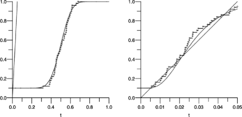
Figure 1: The Simes-line for $\alpha=0.05$ and two realizations of the e.c.d.f. $F_{n}(\cdot|x_{0})$ together with $F_{\infty}(\cdot|x_{0})$ in the D-EX-N$(\zeta_{n})$ model for $n=50$, $\zeta_{n}=0.9$, $\rho=0.95$ and $x_{0}=0.0$ (left picture with $t\in[0,1]$), $x_{0}=-2.0$ (right picture with $t\in[0,0.05]$).

Figure 1 illustrates the enormous impact of the disturbance variable and a large correlation in the D-EX-N$(\zeta_{n})$ model on the LCP determining the number of rejections. In this example, for $x_{0}=0.0$ only the (totally) false hypotheses are rejected, while for $x_{0}=-2.0$ we obtain $38$ false rejections.

Remark 2.2.

Under the assumptions of Lemma 2.1, the Glivenko–Cantelli theorem yields

$$\lim_{n\to\infty}\sup_{t\in[0,1]}\big{|}F_{n}(t|z,\zeta_{n})-F_{\infty}(t|z,\zeta)\big{|}=0\qquad\mbox{almost surely for all }z\in\mathcal{Z}.$$

Moreover,

$$\mathbb{E}[F_{\infty}(t|Z,\zeta)]=\int F_{\infty}(t|z,\zeta)\,dP^{Z}(z)=1-\zeta+\zeta t\qquad\mbox{for all }t\in[0,1].$$

For $\lim_{n\to\infty}\zeta_{n}=\zeta\in(0,1]$, define

$$t(z|\zeta)=\sup\{t\in[\alpha(1-\zeta),\alpha]\dvtx F_{\infty}(t|z,\zeta)=t/\alpha\}.$$ (3)

If there exists an $\epsilon>0$ such that $F_{\infty}(t|z,\zeta)>t/\alpha$ for all $t\in[t(z|\zeta)-\epsilon,t(z|\zeta))$ and $F_{\infty}(t|z,\zeta)<t/\alpha$ for all $t\in(t(z|\zeta),t(z|\zeta)+\epsilon]$, then $t(z|\zeta)$ will be called the largest crossing point (LCP) of $F_{\infty}(\cdot|z,\zeta)$ and the Simes-line. The set of LCP’s will be denoted by $C_{\zeta}$. Moreover, set $D_{\zeta}=\{z\in\mathcal{Z}\dvtx t(z|\zeta)\in C_{\zeta}\}$. Note that there may be some tangent points (TP’s) $t(z|\zeta)$ defined by (3) with $F_{\infty}(t|z,\zeta)\leq t/\alpha$ in a neighborhood of $t(z|\zeta)$. However, it will be assumed that $P^{Z}(D_{\zeta})=1$. In practical examples, $C_{\zeta}$ is a finite union of intervals. For $\zeta\in(0,1)$, we always have a well defined LCP or TP $t(z|\zeta)\geq\alpha(1-\zeta)>0$. For $\zeta=1$, the LCP may be $0$ for a large set of $z$-values, which makes the calculation of the limiting EER and FDR subtler.

In the following we make use of the notation

$$\operatorname{FDR}_{n}(\zeta_{n}|z) = \mathbb{E}\biggl{[}\frac{V_{n}}{R_{n}\vee 1}\Big{|}Z=z\biggr{]},\qquad\operatorname{FDR}_{n}(\zeta_{n})=\mathbb{E}\biggl{[}\frac{V_{n}}{R_{n}\vee 1}\biggr{]},$$

$$\operatorname{FDR}_{\infty}(\zeta|z) = \lim_{n\to\infty}\operatorname{FDR}_{n}(\zeta_{n}|z),\qquad\hskip 4.0pt\operatorname{FDR}_{\infty}(\zeta)=\lim_{n\to\infty}\operatorname{FDR}_{n}(\zeta_{n}),$$

and the corresponding expressions for EER. Moreover, the notation $V_{n}(z)$, $R_{n}(z)$ will be used if $Z=z$ is given.

2.1 All LCP’s greater than zero

We first consider the case $\zeta\in(0,1)$.

Theorem 1.

Given D-EX$(\zeta_{n})$ with $\lim_{n\to\infty}\zeta_{n}=\zeta\in(0,1)$, for all $z\in D_{\zeta}$

$$\lim_{n\to\infty}\frac{V_{n}(z)}{n} = \frac{t(z|\zeta)}{\alpha}-(1-\zeta)\qquad\mbox{a.s.},$$ (4)

$$\lim_{n\to\infty}\frac{V_{n}(z)}{R_{n}(z)\vee 1} = 1-\frac{\alpha(1-\zeta)}{t(z|\zeta)}\qquad\hskip 15.0pt\mbox{a.s.}$$ (5)

With a similar technique as in the proof of Lemma A.2 in r9 , it can be shown that the proportion of rejected hypotheses $R_{n}(z)/n$ converges almost surely to $t(z|\zeta)/\alpha$. This fact immediately implies (4) and (5).

Remark 2.

Under the assumptions of Theorem 1,

$$\operatorname{EER}_{\infty}(\zeta|z) = \mathbb{E}\biggl{[}\lim_{n\to\infty}\frac{V_{n}(z)}{n}\biggr{]}=\frac{t(z|\zeta)}{\alpha}-(1-\zeta),$$ (6)

$$\operatorname{FDR}_{\infty}(\zeta|z) = \mathbb{E}\biggl{[}\lim_{n\to\infty}\frac{V_{n}(z)}{R_{n}(z)\vee 1}\biggr{]}=1-\frac{\alpha(1-\zeta)}{t(z|\zeta)}.$$ (7)

In view of the general assumption $P^{Z}(D_{\zeta})=1$, $z$ can be replaced by $Z$ in (4) and (5).

It remains to calculate $\operatorname{EER}_{\infty}(\zeta)$ and $\operatorname{FDR}_{\infty}(\zeta)$. This may be done in two ways. The first is to integrate (4) and (5) with respect to $P^{Z}$. In this case the main problem is the computation of $t(z|\zeta)$, which can be cumbersome. In general, $t(z|\zeta)$ cannot be determined explicitly. The second possibility seems more convenient and is summarized in the following theorem.

Theorem 3.

Under the assumptions of Theorem 1, suppose that $F_{\infty}(t|z)$ is strictly decreasing in $z$ for $t\in(\alpha(1-\zeta),\alpha)$. Let $C_{\zeta,1}=\{t/\alpha-1+\zeta\dvtx t\in{C}_{\zeta}\}$, $C_{\zeta,2}=\{1-\alpha(1-\zeta)/t\dvtx t\in{C}_{\zeta}\}$ and denote the c.d.f. of$\lim_{n\to\infty}{V_{n}(Z)}/{n}$ and $\lim_{n\to\infty}{V_{n}(Z)}/({R_{n}(Z)\vee 1)}$ by $G_{\zeta,1}$ and $G_{\zeta,2}$, respectively. Then

$$G_{\zeta,1}(u) = 1-W_{Z}\bigl{(}z\bigl{(}\alpha(u+1-\zeta)|\zeta\bigr{)}\bigr{)}\qquad\mbox{for }u\in C_{\zeta,1}\cap(0,\zeta),$$ (8)

$$G_{\zeta,2}(u) = 1-W_{Z}\biggl{(}z\biggl{(}\frac{\alpha(1-\zeta)}{1-u}\Big{|}\zeta\biggr{)}\biggr{)}\qquad\mbox{for }u\in C_{\zeta,2}\cap(0,\zeta),$$ (9)

hence, $\operatorname{EER}_{\infty}$ and $\operatorname{FDR}_{\infty}$ can be computed via

$$\operatorname{EER}_{\infty}(\zeta)=\int_{C_{\zeta,1}}u\,dG_{\zeta,1}(u)\quad\mbox{and}\quad\operatorname{FDR}_{\infty}(\zeta)=\int_{C_{\zeta,2}}u\,dG_{\zeta,2}(u).$$

Let $\zeta\in(0,1)$ and $t\in{C}_{\zeta}\cap(\alpha(1-\zeta),\alpha)$. From (4) in Theorem 1, we get

$$\biggl{\{}z\in D_{\zeta}\dvtx\lim_{n\to\infty}\frac{V_{n}(z)}{n}>\frac{t}{\alpha}-(1-\zeta)\mbox{ a.s. }\biggr{\}}=\{z\in D_{\zeta}\dvtx z<z(t|\zeta)\}.$$

Hence, the substitution $u=t/\alpha-(1-\zeta)$ yields that for all $u\in C_{\zeta,1}\cap(0,\zeta)$

$$W_{Z}\bigl{(}z\bigl{(}\alpha(u+1-\zeta)|\zeta\bigr{)}\bigr{)} = P^{Z}\biggl{(}\biggl{\{}z\in D_{\zeta}\dvtx\lim_{n\to\infty}\frac{V_{n}(z)}{n}>\frac{t}{\alpha}-(1-\zeta)\mbox{ a.s. }\biggr{\}}\biggr{)}$$

$$= 1-G_{\zeta,1}(u),$$

which is (8). Similarly, we obtain from (5) in Theorem 1 that

$$\lim_{n\to\infty}\frac{V_{n}(z)}{R_{n}(z)\vee 1}>1-\frac{\alpha(1-\zeta)}{t}\qquad\mbox{a.s.}\qquad\mbox{iff }z<z(t|\zeta).$$

Therefore, similar arguments as before yield that $G_{\zeta,2}$ is given by (9).

The latter result is a key step for the computation of $\operatorname{EER}_{\infty}(\zeta)$ and $\operatorname{FDR}_{\infty}(\zeta)$. In practical examples it remains to determine the sets $C_{\zeta,1}$ and $C_{\zeta,2}$ and to evaluate the corresponding integrals.

2.2 Some LCP’s equal to zero

If an LCP is equal to zero, the behavior of the FDR heavily depends on the gradient in zero of the c.d.f. of the $p$-value distribution. The next two lemmas cover the finite case.

Lemma 4.

Let $\alpha\in(0,1)$, $0\leq\gamma\leq 1/\alpha$, $n_{0},n\in\mathbb{N}$, $n_{0}\leq n$ and let $\xi_{1},\ldots,\xi_{n_{0}}$ be i.i.d. random variables with values in $[0,1]$ with c.d.f. $F_{\xi}$ satisfying $F_{\xi}(t)=\gamma t$ for all $t\in[0,\alpha]$. Furthermore, let $\xi_{n_{0}+1},\ldots,\xi_{n}$ be random variables with values in $[0,1]$, independent of $(\xi_{j}\dvtx 1\leq j\leq n_{0})$. For $c_{i}=i\alpha/n$, $i=1,\ldots,n$, define $R^{\prime}_{n}=\max\{k\leq n\dvtx\xi_{k:n}\leq c_{k}\}$ and $V^{\prime}_{n}=|\{i\in\{1,\ldots,n_{0}\}\dvtx\xi_{i}\leq c_{R_{n}^{\prime}}\}|$ (with $c_{R_{n}^{\prime}}=-\infty$ for $R_{n}^{\prime}=-\infty$). Then

$$\mathbb{E}\biggl{(}\frac{V^{\prime}_{n}}{R^{\prime}_{n}\vee 1}\biggr{)}=\frac{n_{0}}{n}\gamma\alpha.$$ (10)

For $1\leq i\leq n_{0}$, denote the $(n-1)$-dimensional random vector $(\xi_{1},\ldots,\xi_{i-1},\xi_{i+1},\ldots,\xi_{n})$ by $\xi^{(i)}$, define for $1\leq k<n$ the sets $D_{k}^{(i)}(\alpha)=\{\xi^{(i)}_{k:n-1}>c_{k+1},\ldots,\xi^{(i)}_{n-1:n-1}>c_{n}\}$ and set $D_{0}^{(i)}(\alpha)=\varnothing$, $D_{n}^{(i)}(\alpha)=\Omega$. Then the left-hand side of (10) (cf., e.g., Lemma 3.2 and formula (4.4) in r14 ) is equal to

$$\frac{1}{n}\sum_{i=1}^{n_{0}}\mathrm{P}(\xi_{i}\leq c_{n})+\sum_{i=1}^{n_{0}}\sum_{j=2}^{n}\biggl{[}\frac{\mathrm{P}(\xi_{i}\leq c_{j-1})}{j-1}-\frac{\mathrm{P}(\xi_{i}\leq c_{j})}{j}\biggr{]}\mathrm{P}\bigl{(}D_{j-1}^{(i)}(\alpha)\bigr{)}.$$

Noting that $\mathrm{P}(\xi_{i}\leq c_{n})=\gamma\alpha$ for all $1\leq i\leq n_{0}$ and $\mathrm{P}(\xi_{i}\leq c_{j})/j=\gamma\alpha/n$ for all $1\leq j\leq n$, the assertion follows immediately.

As an application of Lemma 4, we insert a surprising example.

Example 2.1.

Under the general framework of this section, suppose the $X_{i}$ follow an exponential distribution with scale parameter $\lambda=1$ and location parameter $\vartheta_{i}$ and $Z$ follows an exponential distribution with scale parameter $\lambda=1$ and location parameter $0$, and consider the model $T_{i}=g(X_{i},Z)=X_{i}-Z$, $i=1,\ldots,n$. Under $H_{i}\dvtx\vartheta_{i}=0$, the c.d.f. of $T_{i}$ is given by $W_{T}(t)=\exp(t)/2$ for $t\leq 0$ and $W_{T}(t)=1-\exp(-t)/2$ for $t>0$, while the $p$-values (as functions of the observed $z$-value) are given by $p_{i}(z)=1-W_{T}(x_{i}-z)$, $i=1,\ldots,n$. This results in

$$F_{\infty}(t|z)=\cases{2\exp(-z)t,&\quad\mbox{if }$0\leq t\leq 1/2$,\cr\exp(-z)(2-2t)^{-1},&\quad\mbox{if }$1/2<t\leq u(z)$,\cr 1,&\quad\mbox{if }$u(z)<t\leq 1$,}$$

with $u(z)=1-\exp(-z)/2$. For convenience, we restrict attention to the case $\alpha\leq 1/2$. In order to apply Lemma 4, set $F_{\xi}(t)=F_{\infty}(t|z)$ and note that $p_{i}(z)$ has c.d.f. $F_{\xi}$ if $H_{i}$ is true. Therefore, supposing that $n_{0}$ hypotheses are true and $n_{1}=n-n_{0}$ are false with fixed but arbitrary $\vartheta_{i}>0$, we obtain with $\gamma(z)=2\exp(-z)$ and $\zeta_{n}=n_{0}/n$ that $\operatorname{FDR}_{n}(\zeta_{n}|z)=\zeta_{n}\alpha\gamma(z)\mbox{ for all }z>0.$ Integrating with respect to $P^{Z}$ finally results in

$$\operatorname{FDR}_{n}(\zeta_{n})=\zeta_{n}\alpha\int\gamma(z)\,dP^{Z}(z)=\zeta_{n}\alpha.$$

It may be astonishing that the Benjamini–Hochberg upper bound for the FDR is attained for all parameter configurations although the $T_{i}$’s are dependent. Notice that the $\mbox{MTP}_{2}$ property holds in this setting so that the Benjamini–Hochberg bound for the FDR applies. This is a consequence of Propositions 3.7 and 3.8 in karlnott-1980 , because the p.d.f. of the $\operatorname{Exp}(\lambda)$ distribution is $\mbox{PF}_{2}$ for any $\lambda>0$; see karlin-1968 , page 30.

The next result extends Lemma 4 and is a helpful tool in the case that LCP’s are in $0$.

Lemma 5.

Under the assumptions of Lemma 4 but only supposing that $F_{\xi}(t)=\gamma t$ for all $t\in[0,t^{*}]$ for some $t^{*}\in(0,\alpha]$, let $A_{n}(t^{*})=\{F_{n}(t)<t/\alpha\,\forall t\in(t^{*},\alpha]\}$, where $F_{n}$ denotes the e.c.d.f. of $\xi_{1},\ldots,\xi_{n}$. Then, setting $r=\max\{i\in\mathbb{N}_{0}\dvtx i\alpha/n\leq t^{*}\}$,

$$\mathbb{E}\biggl{(}\frac{V^{\prime}_{n}}{R^{\prime}_{n}\vee 1}\mathbf{1}_{A_{n}(t^{*})}\biggr{)}=\frac{n_{0}}{n}\gamma\alpha\mathrm{P}\bigl{(}D_{r}^{(1)}(\alpha)\bigr{)}.$$ (11)

It is clear that $A_{n}(t^{*})=\{R^{\prime}_{n}\leq r\}$; hence, for $r>0$, the left-hand side of (11) is now equal to

$$\frac{1}{r}\sum_{i=1}^{n_{0}}\mathrm{P}(\xi_{i}\leq c_{r})\mathrm{P}\bigl{(}D_{r}^{(i)}(\alpha)\bigr{)}+\sum_{i=1}^{n_{0}}\sum_{j=2}^{r}\biggl{[}\frac{\mathrm{P}(\xi_{i}\leq c_{j-1})}{j-1}-\frac{\mathrm{P}(\xi_{i}\leq c_{j})}{j}\biggr{]}\mathrm{P}\bigl{(}D_{j-1}^{(i)}(\alpha)\bigr{)}.$$

The assertion follows similarly as in the proof of Lemma 4. The following theorem, the proof of which is in the Appendix, is an important step for the understanding of the limiting behavior of both EER (or ENE) and FDR given a fixed value $Z=z$ such that the LCP is in $0$.

Theorem 6.

Given D-EX$(\zeta_{n})$ with $\lim_{n\to\infty}\zeta_{n}=1$, let $z\in\mathcal{Z}$ be such that $F_{\infty}(t|z)<t/\alpha$ for all $t\in(0,\alpha]$. Setting $\gamma(z)=\lim_{t\to 0^{+}}F_{\infty}(t|z)/t,$ it holds that

$$\operatorname{EER}_{\infty}(1|z) = 0,$$ (12)

$$\operatorname{FDR}_{\infty}(1|z) = \alpha\gamma(z).$$ (13)

Remark 7.

In r10 the distribution and expectation of $V_{n}$ were computed for uniform $p$-values under the assumption that all hypotheses are true. Assuming $\zeta_{n}=1$ for all $n\in\mathbb{N}$, the nesting method in the proof of (13) together with the technique in r10 can be used to prove

$$\lim_{n\to\infty}\mathbb{E}[V_{n}(z)]=\cases{\displaystyle\frac{\alpha\gamma(z)}{(1-\alpha\gamma(z))^{2}},&\quad$\gamma(z)<1/\alpha$,\cr\infty,&\quad$\gamma(z)=1/\alpha$.}$$

It is important to note that this formula is only valid for $\zeta_{n}=1$. If $n_{1}$ tends to infinity with $\lim_{n\to\infty}n_{1}/n=0$ and $\gamma(z)>0$, then $\lim_{n\to\infty}\mathbb{E}[V_{n}(z)]=\infty$.

To complete the picture for $\zeta=1$, the next theorem puts things together.

Theorem 8.

Given D-EX$(\zeta_{n})$ with $\lim_{n\to\infty}\zeta_{n}=1$, suppose that $F_{\infty}(t|z)$ is strictly decreasing in $z$ for $t\in(0,\alpha)$. Moreover, let $G_{1,1}$ and $C_{1,1}$ be defined as in Theorem 3 and let $E_{0}=\{z\in\mathcal{Z}\dvtx t(z|1)=0\}$ and $E_{1}=\mathcal{Z}\setminus E_{0}$. Then

$$\operatorname{EER}_{\infty}(1) = \int_{C_{1,1}}u\,dG_{1,1}(u),$$ (14)

$$\operatorname{FDR}_{\infty}(1) = P^{Z}(E_{1})+\alpha\int_{E_{0}}\gamma(z)\,dP^{Z}(z).$$ (15)

Using the disjoint decomposition $\mathcal{Z}=E_{0}+E_{1}$, we obtain

$$\operatorname{EER}_{\infty}(1) = \lim_{n\to\infty}\int_{\mathcal{Z}}\frac{V_{n}(z)}{n}\,dP^{Z}(z)$$

$$= \int_{E_{0}}\lim_{n\to\infty}\frac{V_{n}(z)}{n}\,dP^{Z}(z)+\int_{E_{1}}\lim_{n\to\infty}\frac{V_{n}(z)}{n}\,P^{Z}(z)$$

$$= A_{1}+A_{2}\mbox{ (say)}.$$

Now, Theorem 6 immediately yields $A_{1}=0$, and in analogy to the arguments in the proof of Theorem 3, we get that $A_{2}=\int_{C_{1,1}\setminus\{0\}}u\,dG_{1,1}(u)$. Therefore, (14) is proven. Applying the same decomposition (together with Theorem 6) to $\operatorname{FDR}_{\infty}(1)$ and observing that $\lim_{n\to\infty}V_{n}(z)/(R_{n}(z)\vee 1)=1$ if $z\in E_{1}$ [similar to (5) with $\zeta=1$] finally proves (15).

3 Exchangeable normal variables (Example 2.1 continued)

In the D-EX-N$(\zeta_{n})$ model, assuming that the proportion $\zeta_{n}$ of true null hypotheses tends to 1, we obtain from Lemma 2.1 that the limiting e.c.d.f. of the $p_{i}$’s given $X_{0}=x_{0}$ is given by

$$F_{\infty}(t|x_{0})=1-\Phi\bigl{(}\Phi^{-1}(1-t)/\sqrt{\overline{\rho}}+\sqrt{\rho/\overline{\rho}}x_{0}\bigr{)}\qquad\mbox{for all }t\in(0,1),$$

and $F_{\infty}(0|x_{0})=1-F_{\infty}(1|x_{0})=0$. Note that $F_{\infty}(t|x_{0})=P(\sqrt{\overline{\rho}}X-\break\sqrt{\rho}x_{0}>u_{1-t})$, where $X$ denotes a standard normal variate and $u_{\alpha}$ denotesthe corresponding $\alpha$-quantile. Moreover, it is $\lim_{t\downarrow 0}(\partial/\partial t)F_{\infty}(t|x_{0})=\break\lim_{t\uparrow 1}(\partial/\partial t)F_{\infty}(t|x_{0})=0$, and $F_{\infty}(\cdot|x_{0})$ is convex for $0\leq t\leq\Phi(x_{0}/\sqrt{\rho})$ and concave for $\Phi(x_{0}/\sqrt{\rho})\leq t\leq 1$. Furthermore, $F_{\infty}(t|x_{0})$ is strictly decreasing in $x_{0}$ for $t\in(0,1)$ and $\lim_{\rho\downarrow 0}F_{\infty}(t|x_{0})=t$.

Assuming that $\lim_{n\to\infty}\zeta_{n}=\zeta\in(0,1]$, the limiting e.c.d.f. is given by

$$F_{\infty}(t|x_{0},\zeta)=(1-\zeta)+\zeta F_{\infty}(t|x_{0}).$$

Hence, for $\zeta\in(0,1]$ and given $t\in(0,\alpha)$, $F_{\infty}(t|x_{0},\zeta)=t/\alpha$ iff

$$x_{0}=x_{0}(t|\zeta)=\sqrt{\overline{\rho}/\rho}\Phi^{-1}\bigl{(}(1-t/\alpha)/\zeta\bigr{)}-\Phi^{-1}(1-t)/\sqrt{\rho}.$$ (16)

For $\zeta\in(0,1)$, we get $\lim_{t\downarrow\alpha(1-\zeta)}x_{0}(t|\zeta)=+\infty$ and $\lim_{t\uparrow\alpha}x_{0}(t|\zeta)=-\infty$. Moreover, $F_{\infty}(\cdot|x_{0},\zeta)$ starts above the Simes-line so that there is at least one CP in $(0,1)$. In fact, there may be one, two or three points of intersection in $(0,1)$. For $\zeta=1$, we get in contrast to $\zeta\in(0,1)$ that $\lim_{t\downarrow 0}x_{0}(t|\zeta)=\lim_{t\uparrow\alpha}x_{0}(t|\zeta)=-\infty$. The limiting e.c.d.f. $F_{\infty}(\cdot|x_{0})=F_{\infty}(\cdot|x_{0},1)$ starting with $F_{\infty}(0|x_{0})=0$ may have no, one or two CP’s in $(0,1)$.

In order to determine the set of LCP’s, the following derivations are helpful. Let $u=\Phi^{-1}(1-t)$ and let

$$\hskip 20.0ptd(u|x_{0},\zeta)=(1-\zeta)+\zeta\bigl{(}1-\Phi\bigl{(}u/\sqrt{\overline{\rho}}+\sqrt{\rho/\overline{\rho}}x_{0}\bigr{)}\bigr{)}-\bigl{(}1-\Phi(u)\bigr{)}/\alpha$$ (17)

denote the distance between the transformed $F_{\infty}$-curve and the transformed Simes-line. Then the conditions

$$d(u|x_{0},\zeta) = 0,$$ (18)

$$\frac{\partial}{\partial u}d(u|x_{0},\zeta) = 0$$ (19)

are necessary and sufficient for a TP ($F_{\infty}$ touches the Simes-line). Note that condition (19) is equivalent to

$$u\in\bigl{\{}u_{1,2}(x_{0})=-x_{0}/\sqrt{\rho}\pm\sqrt{\overline{\rho}/\rho}\sqrt{x_{0}^{2}-2\ln(\sqrt{\overline{\rho}}/(\alpha\zeta))}\bigr{\}}.$$ (20)

If there exists a real solution $u^{*}$ of (18) and $u^{*}=u_{2}(x_{0})=-x_{0}/\sqrt{\rho}-\sqrt{\overline{\rho}/\rho}\times\break\sqrt{x_{0}^{2}-2\ln(\sqrt{\overline{\rho}}/(\alpha\zeta))}$ for given values of $x_{0},\rho,\zeta$, then we define $t_{2}=\break 1-\Phi(u^{*})$. If such a solution $u^{*}$ exists in case of $\zeta\in(0,1)$, define $t_{1}$ as the smaller solution of $F_{\infty}(t|x_{0},\zeta)=t/\alpha$. Then the set of LCP’s is given by $C_{\zeta}=(\alpha(1-\zeta),t_{1})\cup(t_{2},\alpha)$. Note that for $\zeta=1$ there exists a unique TP such that the set of LCP’s is given by $C_{\zeta}=\{0\}\cup(t_{2},\alpha)$. Furthermore, for $\zeta\in(0,1)$, there may be no such TP. In the latter case, formally interpreted as $t_{1}=t_{2}$, we have $C_{\zeta}=(\alpha(1-\zeta),\alpha)$. For example, such a situation occurs in the case $\overline{\rho}\geq(\alpha\zeta)^{2}$ and $\alpha\in(0,1/2]$ iff $d(u_{2}(\underline{x}_{0})|\underline{x}_{0},\zeta)\geq 0$ for $\underline{x}_{0}=-\sqrt{2\ln(\sqrt{\overline{\rho}}/(\alpha\zeta))}$.

The (discontinuous) case $t_{1}<t_{2}$ looks somewhat paradoxical. In this case, depending on the observed $x_{0}$, either a small proportion $\pi_{1}\in((1-\zeta),t_{1}/\alpha)$ or a larger proportion $\pi_{2}\in(t_{2}/\alpha,1)$ of hypotheses will be rejected although the distance between the corresponding $x_{0}$ values may be small. This occurs, for example, for $\alpha=0.1$, $\zeta=0.9999$.

The following two theorems give formulas for $\operatorname{EER}_{\infty}$ and $\operatorname{FDR}_{\infty}$. The first theorem covers $\zeta\in(0,1)$, the second one $\zeta=1$. The proof of Theorem 9 can be found in the Appendix, while the proof of Theorem 10 is a straightforward application of Theorem 8.

Theorem 9.

Given model D-EX-N$(\zeta_{n})$ with $\lim_{n\to\infty}\zeta_{n}=\zeta\in(0,1)$, the set of LCP’s is $C_{\zeta}=(\alpha(1-\zeta),t_{1})\cup(t_{2},\alpha)$ for $t_{1}<t_{2}$ and $C_{\zeta}=(\alpha(1-\zeta),\alpha)$ for $t_{1}=t_{2}$ (i.e., no TP) and

$$\operatorname{EER}_{\infty}(\zeta) = \frac{t_{2}-t_{1}}{\alpha}\Phi(x_{0}(t_{1}|\zeta))$$

$${}+\int_{1-\zeta}^{t_{1}/\alpha}\Phi(x_{0}(\alpha t|\zeta))\,dt+\int_{t_{2}/\alpha}^{1}\Phi(x_{0}(\alpha t|\zeta))\,dt,$$

$$\operatorname{FDR}_{\infty}(\zeta) = (z_{2}-z_{1})\Phi\biggl{(}x_{0}\biggl{(}\frac{\alpha(1-\zeta)}{1-z_{1}}\Big{|}\zeta\biggr{)}\biggr{)}$$

$${}+\int_{0}^{z_{1}}\Phi\biggl{(}x_{0}\biggl{(}\frac{\alpha(1-\zeta)}{1-z}\Big{|}\zeta\biggr{)}\biggr{)}\,dz+\int_{z_{2}}^{\zeta}\Phi\biggl{(}x_{0}\biggl{(}\frac{\alpha(1-\zeta)}{1-z}\Big{|}\zeta\biggr{)}\biggr{)}\,dz,$$

where $z_{i}=1-\alpha(1-\zeta)/t_{i}$ , $i=1,2$.

Theorem 10.

Given model D-EX-N$(\zeta_{n})$ with $\lim_{n\to\infty}\zeta_{n}=\zeta=1$, the set of LCP’s is $C_{\zeta}=\{0\}\cup(t_{2},\alpha)$ and

$$\operatorname{EER}_{\infty}(1) = t_{2}\Phi(x_{0}(t_{2}|\zeta))/\alpha+\int_{t_{2}/\alpha}^{1}\Phi(x_{0}(\alpha t|\zeta))\,dt,$$

$$\operatorname{FDR}_{\infty}(1) = \Phi(x_{0}(t_{2}|\zeta)).$$

Remark 11.

For $\zeta=1$, we obtain an upper bound for $x_{0}(t_{2}|\zeta)$ and $\operatorname{FDR}_{\infty}(1)$, respectively, if $\rho\leq 1-\alpha^{2}$. From the derivations before Theorem 9, we get $x_{0}(t_{2}|\zeta)\leq\underline{x}_{0}=-\sqrt{2\ln(\sqrt{\overline{\rho}}/\alpha)}$ and consequently, $\operatorname{FDR}_{\infty}(1)\leq\Phi(\underline{x}_{0})$. This is helpful for the numerical determination of $x_{0}(t_{2}|\zeta)$.

The following interesting and maybe unexpected result, which will be discussed in Section 5, concerns a discontinuity for $\zeta=1$ and $\rho\to 0$. The proof is given in the Appendix.

Theorem 12.

Given model D-EX-N$(\zeta_{n})$ with $\lim_{n\to\infty}\zeta_{n}=\zeta=1$ and $\alpha\in(0,1/2]$,

$$\lim_{\rho\to 0^{+}}\operatorname{FDR}_{\infty}(1)=\Phi\bigl{(}-\sqrt{-2\ln(\alpha)}\bigr{)}.$$ (21)

Figure 2: $\operatorname{EER}_{\infty}(\zeta)$ in the D-EX-N$(\zeta_{n})$ model for $\alpha=0.05$ and $\zeta=0.1,~{}0.2,~{}0.3,~{}0.4,~{}0.5$ (left picture) and $\zeta=0.6,~{}0.7,~{}0.8,~{}0.9,~{}0.95,~{}0.975,~{}1$ (right picture).

Figure 3: $\operatorname{FDR}_{\infty}(\zeta)$ in the D-EX-N$(\zeta_{n})$ model for $\alpha=0.05$ and $\zeta=0.1,~{}0.2,~{}0.4,~{}0.6,~{}0.8,$ $0.9$ (left picture) and $\zeta=0.95,~{}0.96,~{}0.97,~{}0.98,~{}0.99,~{}0.995,~{}0.999,~{}0.9999,~{}0.99999,~{}1$ (right picture).

Figures 2 and 3 display $\operatorname{EER}_{\infty}(\zeta)$ and $\operatorname{FDR}_{\infty}(\zeta)$, respectively, for various values of $\zeta$ for $\rho\in[0,1]$. For $\rho\to 0$, $\operatorname{EER}_{\infty}(\zeta)$ tends to $\alpha(1-\zeta)/(1-\alpha\zeta)$ as expected (cf. r9 ) and for $\rho\to 1$, $\operatorname{EER}_{\infty}(\zeta)$ tends to $\zeta\alpha$. Moreover, it seems that $\operatorname{EER}_{\infty}(\zeta)$ is increasing in $\rho$ with largest values for large $\rho$ and $\zeta$. If $\rho$ is not too large ($<0.9$), $\operatorname{EER}_{\infty}(\zeta)$ is largest for $\zeta\approx 1/2$. For $\zeta\in(0,1)$, FDR tends to the Benjamini–Hochberg bound for $\rho\to 0$ and $\rho\to 1$. For $\rho=1$, we have total dependence so that $\operatorname{FDR}_{n}(\zeta_{n})=\zeta_{n}\alpha$ in the D-EX-N$(\zeta_{n})$ model. For large values of $\zeta$, the computation of $\operatorname{FDR}_{\infty}(\zeta)$ is extremely cumbersome. The main reason is that the TP’s are very close to 0 so that an enormous numerical accuracy is required. Finally, it is interesting to note that for $\zeta=1$, $\operatorname{FDR}_{\infty}(1)$ reflects the limiting behavior of the true level of Simes’ r17 global test for the intersection hypothesis. Our results imply that this global test has an asymptotic level greater than zero for all correlations $\rho\in[0,1]$, which is a new finding.

4 Studentized normal variables (Example 2.2 continued)

In the D-EX-t$(\zeta_{n})$ model with $\lim_{n\rightarrow\infty}\zeta_{n}=\zeta=1$, $F_{\infty}(\cdot|s)$ is given by

$$F_{\infty}(t|s)=1-\Phi\bigl{(}sF_{t_{\nu}}^{-1}(1-t)\bigr{)}=1-\Phi(st_{\nu,1-t}).$$

Note that $F_{\infty}(t|s)$ is decreasing in $s$ for $t<1/2$ and increasing in $s$ for $t>1/2$. Moreover, $(\partial/\partial t)F_{\infty}(t|s)=s\varphi(st_{\nu,1-t})/f_{t_{\nu}}(t_{\nu,1-t}),$ hence, we get $\lim_{t\downarrow 0}(\partial/\partial t)F_{\infty}(t|s)=$ $\lim_{t\uparrow 1}(\partial/\partial t)F_{\infty}(t|s)=0$. Moreover,

$$\frac{\partial^{2}}{\partial t^{2}}F_{\infty}(t|s)>0\qquad\mbox{iff }-s^{2}t_{\nu,1-t}<\frac{f_{t_{\nu}}^{\prime}(t_{\nu,1-t})}{f_{t_{\nu}}(t_{\nu,1-t})}.$$

This condition is equivalent to

$$s^{2}t_{\nu,1-t}>\frac{\nu+1}{\nu}\biggl{(}1+\frac{t_{\nu,1-t}^{2}}{\nu}\biggr{)}^{-1}t_{\nu,1-t}.$$

Hence, for $t<1/2$, $F_{\infty}(t|s)$ is convex for $t<\min\{1/2,F_{t_{\nu}}(-a(s,\nu))\}$ with $a(s,\nu)=((\nu+1)/s^{2}-\nu)^{1/2}$ and concave otherwise. For $t>1/2$, $F_{\infty}(t|s)$ is convex for $t<\max\{1/2,F_{t_{\nu}}(a(s,\nu))\}$ and concave otherwise. Notice that $F_{\infty}(1/2|s)=1/2$ for all $s>0$. As a consequence, for $\alpha<1/2$, $F_{\infty}$ crosses the Simes-line at most if $F_{t_{\nu}}(-a(s,\nu))<1/2$, which happens if $s^{2}<(\nu+1)/\nu$.

Given the D-EX-t$(\zeta_{n})$ model with $\lim_{n\to\infty}\zeta_{n}=\zeta\in(0,1]$, the limiting e.c.d.f. is given by

$$F_{\infty}(t|s,\zeta)=(1-\zeta)+\zeta\bigl{(}1-\Phi\bigl{(}sF_{t_{\nu}}^{-1}(1-t)\bigr{)}\bigr{)}.$$

For convenience, we restrict attention to $\alpha\in(0,1/2]$ in the remainder of this section. For $\zeta\in(0,1]$, we have $F_{\infty}(t|s,\zeta)=t/\alpha$ iff

$$s=s(t|\zeta)=\frac{\Phi^{-1}((1-t/\alpha)/\zeta)}{F_{t_{\nu}}^{-1}(1-t)},$$

where $s(t|\zeta)>0$ iff $t<\alpha(1-\zeta/2)$. Therefore, LCP’s are only possible in $[t_{u},t_{o}]$ with $t_{u}=\alpha(1-\zeta)$ and $t_{o}=\alpha(1-\zeta/2)$. Notice that $\lim_{t\downarrow t_{u}}s(t|\zeta)=\lim_{t\uparrow t_{o}}s(t|\zeta)=0$ for $\zeta=1$, while $\lim_{t\downarrow t_{u}}s(t|\zeta)=\infty$ and $\lim_{t\uparrow t_{o}}s(t|\zeta)=0$ for $\zeta\in(0,1)$. For $\zeta\in(0,1)$, the set $C_{\zeta}$ of LCP’s consists of one or two intervals denoted by $(\alpha(1-\zeta),t_{1})$ and $(t_{2},\alpha(1-\zeta/2))$. If there exists a TP we have $t_{1}<t_{2}$ and the TP is $t_{2}$; otherwise $t_{1}=t_{2}$. In the case $\zeta=1$ the existence of a TP (denoted by $t_{2}$) is guaranteed and the set of LCP’s is given by $C_{1}=\{0\}\cup(t_{2},\alpha/2)$. Hence, the situation is quite similar to the D-EX-N$(\zeta_{n})$ model in Section 3 except that there are no crossing points at all in $[t_{o},\alpha]$. With $u=F_{t_{\nu}}^{-1}(1-t)$, the distance function between $F_{\infty}$ and the Simes-line is defined by $d_{\nu}(u|s,\zeta)=(1-\zeta)+\zeta(1-\Phi(su))-F_{t_{\nu}}(-u)/\alpha.$ Necessary and sufficient conditions for a TP ($F_{\infty}$ touches the Simes-line) are now given by

$$d_{\nu}(u|s,\zeta)=0\quad\mbox{and}\quad\frac{\partial}{\partial u}d_{\nu}(u|s,\zeta)=0,$$

which are equivalent to $\alpha\Phi(-su)=F_{t_{\nu}}(-u)$ and $s\alpha\varphi(su)=f_{t_{\nu}}(u)$.

We summarize the behavior of EER and FDR in the following two theorems in analogy to the results of Section 3.

Theorem 13.

Given model D-EX-t$(\zeta_{n})$ with $\lim_{n\to\infty}\zeta_{n}=\zeta\in(0,1)$ and $\alpha\in(0,1/2]$, the set of LCP’s is $C_{\zeta}=(\alpha(1-\zeta),t_{1})\cup(t_{2},\alpha(1-\zeta/2))$ for $t_{1}<t_{2}$ and $C_{\zeta}=(\alpha(1-\zeta),\alpha(1-\zeta/2))$ for $t_{1}=t_{2}$ (i.e., no TP) and

$$\operatorname{EER}_{\infty}(\zeta) = \frac{t_{2}-t_{1}}{\alpha}F_{\chi_{\nu}}\bigl{(}\sqrt{\nu}s(t_{1}|\zeta)\bigr{)}$$

$${}+\int_{1-\zeta}^{t_{1}/\alpha}F_{\chi_{\nu}}\bigl{(}\sqrt{\nu}s(\alpha t|\zeta)\bigr{)}\,dt$$

$${}+\int_{t_{2}/\alpha}^{1-\zeta/2}F_{\chi_{\nu}}\bigl{(}\sqrt{\nu}s(\alpha t|\zeta)\bigr{)}\,dt,$$

$$\operatorname{FDR}_{\infty}(\zeta) = (z_{2}-z_{1})F_{\chi_{\nu}}\biggl{(}\sqrt{\nu}s\biggl{(}\frac{\alpha(1-\zeta)}{1-z_{1}}\Big{|}\zeta\biggr{)}\biggr{)}$$

$${}+\int_{0}^{z_{1}}F_{\chi_{\nu}}\biggl{(}\sqrt{\nu}s\biggl{(}\frac{\alpha(1-\zeta)}{1-z}\Big{|}\zeta\biggr{)}\biggr{)}\,dz$$

$${}+\int_{z_{2}}^{z_{3}}F_{\chi_{\nu}}\biggl{(}\sqrt{\nu}s\biggl{(}\frac{\alpha(1-\zeta)}{1-z}\Big{|}\zeta\biggr{)}\biggr{)}\,dz,$$

where $z_{i}=1-\alpha(1-\zeta)/t_{i}$ , $i=1,2$, and $z_{3}=\zeta/(2-\zeta)$.

Theorem 14.

Given model D-EX-t$(\zeta_{n})$ with $\lim_{n\to\infty}\zeta_{n}=\zeta=1$ and $\alpha\in(0,1/2]$, the set of LCP’s is $C_{\zeta}=\{0\}\cup(t_{2},\alpha/2)$ and

$$\operatorname{EER}_{\infty}(1) = t_{2}F_{\chi_{\nu}}\bigl{(}\sqrt{\nu}s(t_{2}|\zeta)\bigr{)}/\alpha+\int_{t_{2}/\alpha}^{1}F_{\chi_{\nu}}\bigl{(}\sqrt{\nu}s(\alpha t|\zeta)\bigr{)}\,dt,$$

$$\operatorname{FDR}_{\infty}(1) = F_{\chi_{\nu}}\bigl{(}\sqrt{\nu}s(t_{2}|\zeta)\bigr{)}.$$

Finally, for $\zeta=1$, we consider the case that the degrees of freedom $\nu$ tend to infinity. Heuristically, this means that the model tends to independence. In contrast to the normal case of the previous section, the solution is more difficult. The reason is that one has to find suitable asymptotic expansions for $f_{t_{\nu}}$ and $F_{t_{\nu}}$ given in r4fd . Application of these expansions yields the following result, the proof of which is given in the Appendix.

Lemma 15.

Let $\alpha\in(0,1/2]$ and define

$$s=s_{\nu}(x)=1-\nu^{-1/2}(-\ln(x))^{1/2}+o(\nu^{-1/2}),\qquad x\in(0,1/2].$$

Then, given model D-EX-t$(\zeta_{n})$ with $\lim_{n\to\infty}\zeta_{n}=\zeta=1$, it holds for sufficiently large $\nu$ that $F_{\infty}(\cdot|s_{\nu}(x))$ has (i) two CP’s for all $x\in(0,\alpha)$, and (ii) no CP for all $x\in(\alpha,1/2]$.

Application of this lemma yields the same limit of the FDR for $\zeta_{n}\to 1$ and $\nu\to\infty$ as in Theorem 12; cf. the discussion in Section 5.

Theorem 16.

Let $\alpha\in(0,1/2]$. Then, given model D-EX-t$(\zeta_{n})$ with$\lim_{n\to\infty}\zeta_{n}=1$,

$$\lim_{\nu\to\infty}\operatorname{FDR}_{\infty}(1)=\Phi\bigl{(}-\sqrt{-2\ln(\alpha)}\bigr{)}.$$ (22)

The result follows by letting $x\to\alpha$ in Lemma 15 and by applying the central limit theorem. Setting $s_{\nu}=s_{\nu}(\alpha)$, we get

$$\lim_{\nu\to\infty}\operatorname{FDR}_{\infty}(1) = \lim_{\nu\to\infty}P(S\leq s_{\nu})$$

$$= \lim_{\nu\to\infty}P\biggl{(}\frac{\nu S^{2}-\nu}{\sqrt{2\nu}}\leq\frac{\nu s_{\nu}^{2}-\nu}{\sqrt{2\nu}}\biggr{)}$$

$$= \lim_{\nu\to\infty}P\biggl{(}\frac{\nu S^{2}-\nu}{\sqrt{2\nu}}\leq-\sqrt{-2\ln(\alpha)}+o(1)\biggr{)}$$

$$= \Phi\bigl{(}-\sqrt{-2\ln(\alpha)}\bigr{)}.$$

Figure 4: $\operatorname{EER}_{\infty}(\zeta)$ in the D-EX-t$(\zeta_{n})$ model for $\alpha=0.05$ and $\zeta=0.1,~{}0.2,~{}0.3,~{}0.4,~{}0.5$ (left picture) and $\zeta=0.6,~{}0.7,~{}0.8,~{}0.9,~{}0.95,~{}0.975,~{}1$ (right picture).

In analogy to Section 3, Figures 4 and 5 display $\operatorname{EER}_{\infty}(\zeta)$ and $\operatorname{FDR}_{\infty}(\zeta)$, respectively, for various values of $\zeta$ and $\nu$. It seems that $\operatorname{EER}_{\infty}(\zeta)$ is decreasing in $\nu$. For $\nu\to\infty$, $\operatorname{EER}_{\infty}(\zeta)$ again tends to the value $\alpha(1-\zeta)/(1-\alpha\zeta)$ as expected; see r9 . Note that $\operatorname{EER}_{\infty}(\zeta)$ is already close to this limit if $\nu$ is not too small. As expected, for $\zeta\approx 1/2$ and $\nu$ not too small, $\operatorname{EER}_{\infty}(\zeta)$ is largest. Except for $\zeta=1$, the FDR tends to the Benjamini–Hochberg bound $\zeta\alpha$ for increasing degrees of freedom. The limit for $\nu\to 0$ is not clear. In the latter case the density of the $t$-distribution becomes flatter and flatter and the computation of $\operatorname{FDR}_{\infty}(\zeta)$ becomes extremely difficult. As in the D-EX-N$(\zeta_{n})$ model with $\zeta_{n}\to 1$, $\operatorname{FDR}_{\infty}(1)$ reflects the limiting behavior of the true level of Simes’ r17 global test for the intersection hypothesis and again, our results show that it is asymptotically greater than zero for all $\nu>0$.

Figure 5: $\operatorname{FDR}_{\infty}(\zeta)$ in the D-EX-t$(\zeta_{n})$ model for $\alpha=0.05$ and $\zeta=0.1,0.2,0.4,0.6,0.8,0.9$ (left picture) and $\zeta=0.9,~{}0.95,~{}0.99,~{}0.999,~{}0.9999,~{}1$ (right picture).

5 Concluding remarks

The investigations in this paper show that the false discovery proportion FDP$=V_{n}/[R_{n}\vee 1]$ of the LSU-procedure can be very volatile in the case of dependent $p$-values, that is, the actual FDP may be much larger (or smaller) than in the independent case. The same is true for $V_{n}$, $V_{n}/n$, $R_{n}$ and $R_{n}/n$. Under mild assumptions, the e.c.d.f. of the $p$-values converges to a fixed curve under independence (cf. r9 ), which implies convergence of $V_{n}/n$ and $R_{n}/n$ to fixed values. On the other hand, the shape of the e.c.d.f. of the $p$-values under exchangeability heavily depends on the (realization of the) disturbance variable $Z$; cf. Figure 1. In the latter case, the limit distribution of $V_{n}/n$ and $R_{n}/n$ typically has positive variance.

It is often assumed that there may be some kind of weak dependence between test statistics (cf., e.g., r22 ), being close to independence in some sense. The results in Theorems 12 and 16 and the numerical calculations reflected in Figures 3 and 5 suggest that for large $n$ and $\zeta_{n}\rightarrow 1$ small deviations from independence (small $\rho$ or large $\nu$) may result in a substantially smaller FDR than the Benjamini–Hochberg bound. However, simulations for small $\rho$ and large $\nu$ show that $\operatorname{FDR}_{n}(\zeta_{n})$ approaches its limit $\operatorname{FDR}_{\infty}(1)$ only for unrealistically large values of $n$ if $\zeta_{n}\rightarrow 1$. For example, in the D-EX-N$(\zeta_{n})$ model with $\alpha=0.05$, $n=100{,}000$ and $\rho=0.1$, we obtained $\operatorname{FDR}_{n}(1)\approx 0.0417$ by simulation. For $\rho=0.01$, we got $\operatorname{FDR}_{n}(1)\approx 0.05$. A possible explanation may be that $\lim_{\rho\rightarrow 0^{+}}\operatorname{FDR}_{n}(1)=\alpha$, $\lim_{\nu\rightarrow\infty}\operatorname{FDR}_{n}(1)=\alpha$, hence, the order of limits plays a severe role. Moreover, for small $\rho$, it seems that $n$ has to be very large such that the e.c.d.f. reproduces the shape of $F_{\infty}$ close to $0$. For $\zeta<1$, the $\operatorname{FDR}_{\infty}$ curves in Figures 3 and 5 reflect the FDR for realistically large $n$ (e.g., $n=1000$) very well. The reason is that the shape behavior of $F_{\infty}$ close to $0$ is not that crucial as for $\zeta=1$.

Example 2.1 shows that the FDR under dependence may also have the same behavior as in the independent case. Therefore, it seems very difficult to predict what happens with EER, FDR and FDP in models with more complicated dependence structure, for example, in a multivariate normal model with arbitrary covariance matrix. In any case, results of the LSU-procedure, or more generally, of any FDR controlling procedure, should be interpreted with some care under dependence, taking into account that the FDR refers to an expectation and that the procedure at hand may lead to much more false discoveries than expected.

In the models studied in Sections 3 and 4, the EER becomes smallest if $\vartheta_{i}\rightarrow 0^{+}$ for all $i\in I_{1}$ and tends to $\zeta_{n}\operatorname{EER}_{n}(1)$, where $I_{1}=\{j\dvtx K_{j}\ni\vartheta_{j}\}$. It is not clear for which parameters $\vartheta_{i}$ the FDR becomes smallest. However, if $\vartheta_{i}\rightarrow 0^{+}$ for all $i\in I_{1}$, $\zeta_{n}\rightarrow\zeta\in(0,1)$, the FDR tends to $\zeta\operatorname{FDR}_{\infty}(1)$.

Finally, with slight modifications of the methods developed in this paper, one can also treat statistics like $T_{i}=|X_{i}-Z|$ or $T_{i}=|X_{i}|/Z$. Somewhat more effort will be necessary if the disturbance variable $Z$ is two-dimensional as, for example, in $T_{i}=|X_{i}-Z_{1}|/Z_{2}$.

Appendix: Proofs

Proof of Theorem 6 The assumptions concerning $F_{\infty}$ imply that $\lim_{n\to\infty}R_{n}(z)/n=0$ almost surely. Noting that $V_{n}(z)/n\leq R_{n}(z)/n$ for all $n\in\mathbb{N}$, (12) is obvious.

In order to prove (13), we nest $F_{\infty}$ between two c.d.f.’s being linear in a neighborhood of zero. To this end, let $t^{*}\in(0,\alpha]$ be fixed, $B=[0,t^{*})$, $m_{\ell}(t^{*})=\inf_{t\in B\setminus\{0\}}F_{\infty}(t|z)/t$, $m_{u}(t^{*})=\sup_{t\in B\setminus\{0\}}F_{\infty}(t|z)/t$, and

$$F_{\ell}(t) = m_{\ell}(t^{*})t\cdot\mathbf{1}_{B}(t)+F_{\infty}(t|z)\cdot\mathbf{1}_{B^{c}}(t),$$

$$F_{u}(t) = m_{u}(t^{*})t\cdot\mathbf{1}_{B}(t)+\max\{m_{u}(t^{*})t^{*},F_{\infty}(t|z)\}\cdot\mathbf{1}_{B^{c}}(t).$$

This results in $F_{\ell}(t)\leq F_{\infty}(t|z)\leq F_{u}(t)$ for all $t\in[0,1]$. For $n\in\mathbb{N}$, let the event $A_{n}(t^{*})$ be defined as in Lemma 5. Then

$$\operatorname{FDR}_{n}(\zeta_{n}|z) = \mathbb{E}\biggl{(}\frac{V_{n}(z)}{R_{n}(z)\vee 1}\mathbf{1}_{A_{n}(t^{*})}\biggr{)}+\mathbb{E}\biggl{(}\frac{V_{n}(z)}{R_{n}(z)\vee 1}\mathbf{1}_{A^{c}_{n}(t^{*})}\biggr{)}$$

$$= \Lambda_{n}+\lambda_{n}\mbox{ (say)}.$$

With $r_{n}=\max\{i\in\mathbb{N}_{0}\dvtx i\alpha/n\leq t^{*}\}$, we obtain similarly to the arguments in the proof of Lemma 4 that

$$\Lambda_{n} = \mathbb{E}\biggl{(}\frac{V_{n}(z)}{R_{n}(z)\vee 1}\mathbf{1}_{\{R_{n}(z)\leq r_{n}\}}\biggr{)}$$

$$= n_{0}\sum_{j=1}^{r_{n}}\frac{\mathrm{P}(p_{1}(z)\leq j\alpha/n)}{j}\bigl{[}\mathrm{P}\bigl{(}D_{j}^{(1)}(\alpha)\bigr{)}-\mathrm{P}\bigl{(}D_{j-1}^{(1)}(\alpha)\bigr{)}\bigr{]}.$$

Due to the pointwise order of $F_{\ell}$, $F_{\infty}$ and $F_{u}$, we get

$$\zeta_{n}m_{\ell}(t^{*})\alpha\mathrm{P}\bigl{(}D_{r_{n}}^{(1)}(\alpha)\bigr{)} \leq \Lambda_{n}\leq\zeta_{n}m_{u}(t^{*})\alpha\mathrm{P}\bigl{(}D_{r_{n}}^{(1)}(\alpha)\bigr{)},$$

$$\zeta_{n}m_{\ell}(t^{*})\alpha\mathrm{P}\bigl{(}D_{r_{n}}^{(1)}(\alpha)\bigr{)}+\lambda_{n} \leq \operatorname{FDR}_{n}(\zeta_{n}|z)\leq\zeta_{n}m_{u}(t^{*})\alpha\mathrm{P}\bigl{(}D_{r_{n}}^{(1)}(\alpha)\bigr{)}+\lambda_{n}.$$

Since $\zeta_{n}\to 1$, $\mathrm{P}(D_{r_{n}}^{(1)}(\alpha))\to 1$ and $\mathrm{P}(A_{n}(t^{*}))\to 1$ for $n\to\infty$, we obtain $\lambda_{n}\to 0$ and $m_{\ell}(t^{*})\alpha\leq\lim\inf_{n\to\infty}\operatorname{FDR}_{n}(\zeta_{n}|z)\leq\lim\sup_{n\to\infty}\operatorname{FDR}_{n}(\zeta_{n}|z)$ $\leq\break m_{u}(t^{*})\alpha$. The assertion now follows by noticing that $\lim_{t^{*}\to 0^{+}}m_{\ell}(t^{*})=\break\lim_{t^{*}\to 0^{+}}m_{u}(t^{*})=\gamma(z)$.

Proof of Theorem 9 Denote the p.d.f. corresponding to $G_{\zeta,1}$ by $g_{\zeta,1}$ and notice that $C_{\zeta,1}=(0,t_{1}/\alpha-(1-\zeta))\cup(t_{2}/\alpha-(1-\zeta),\zeta)$. From Theorem 3, we get

$$\operatorname{EER}_{\infty}(\zeta)=\int_{0}^{t_{1}/\alpha-(1-\zeta)}ug_{\zeta,1}(u)\,du+\int_{t_{2}/\alpha-(1-\zeta)}^{\zeta}ug_{\zeta,1}(u)\,du.$$

Since $x_{0}(t_{1}|\zeta)=x_{0}(t_{2}|\zeta)$ and $\lim_{t\uparrow\alpha}x_{0}(t|\zeta)=-\infty$, we get

$$\operatorname{EER}_{\infty}(\zeta) = \bigl{(}t_{1}/\alpha-(1-\zeta)\bigr{)}\bigl{(}1-\Phi(x_{0}(t_{1}|\zeta))\bigr{)}+\zeta$$

$${}-\bigl{(}t_{2}/\alpha-(1-\zeta)\bigr{)}\bigl{(}1-\Phi(x_{0}(t_{1}|\zeta))\bigr{)}-\bigl{(}t_{1}/\alpha-(1-\zeta)\bigr{)}-\zeta$$

$${}+t_{2}/\alpha-(1-\zeta)+\int_{0}^{t_{1}/\alpha-(1-\zeta)}\Phi\bigl{(}x_{0}\bigl{(}\alpha(u+1-\zeta)|\zeta\bigr{)}\bigr{)}\,du$$

$${}+\int_{t_{2}/\alpha-(1-\zeta)}^{\zeta}\Phi\bigl{(}x_{0}\bigl{(}\alpha(u+1-\zeta)|\zeta\bigr{)}\bigr{)}\,du$$

$$= \frac{t_{2}-t_{1}}{\alpha}\Phi(x_{0}(t_{1}|\zeta))$$

$${}+\int_{1-\zeta}^{t_{1}/\alpha}\Phi(x_{0}(\alpha t|\zeta))\,dt+\int_{t_{2}/\alpha}^{1}\Phi(x_{0}(\alpha t|\zeta))\,dt.$$

In order to compute $\operatorname{FDR}_{\infty}(\zeta)$, note that, for $z\in(0,z_{1})\cup(z_{2},\zeta)$,

$$G_{\zeta,2}(z)=1-\Phi\biggl{(}x_{0}\biggl{(}\frac{\alpha(1-\zeta)}{1-z}\Big{|}\zeta\biggr{)}\biggr{)},$$

where $z_{i}=1-\alpha(1-\zeta)/t_{i}$ , $i=1,2$. In view of $\lim_{t\downarrow\alpha(1-\zeta)}x_{0}(t|\zeta)=\infty$, it is $G_{\zeta,2}(z_{1})=G_{\zeta,2}(z_{2})$, $G_{\zeta,2}(0)=0$ and $G_{\zeta,2}(\zeta)=1$. Denoting the corresponding p.d.f. of $G_{\zeta,2}$ by $g_{\zeta,2}$, we obtain

$$\operatorname{FDR}_{\infty}(\zeta) = \int_{0}^{z_{1}}zg_{\zeta,2}(z)\,dz+\int_{z_{2}}^{\zeta}zg_{\zeta,2}(z)\,dz$$

$$= z_{1}G_{\zeta,2}(z_{1})+\zeta G_{\zeta,2}(\zeta)-z_{2}G_{\zeta,2}(z_{2})$$

$${}-\int_{0}^{z_{1}}G_{\zeta,2}(z)\,dz-\int_{z_{2}}^{\zeta}G_{\zeta,2}(z)\,dz$$

$$= (z_{2}-z_{1})\Phi\biggl{(}x_{0}\biggl{(}\frac{\alpha(1-\zeta)}{1-z_{1}}\Big{|}\zeta\biggr{)}\biggr{)}$$

$${}+\int_{0}^{z_{1}}\Phi\biggl{(}x_{0}\biggl{(}\frac{\alpha(1-\zeta)}{1-z}\Big{|}\zeta\biggr{)}\biggr{)}\,dz$$

$${}+\int_{z_{2}}^{\zeta}\Phi\biggl{(}x_{0}\biggl{(}\frac{\alpha(1-\zeta)}{1-z}\Big{|}\zeta\biggr{)}\biggr{)}\,dz.$$

Proof of Theorem 12 For any $\rho\in(0,1)$, there exists a unique solution $(u,x_{0})=(u_{\rho},x_{0,\rho})$ (say) of (18) and (19). In view of (20) and the shape of $F_{\infty}$, $(u_{\rho},x_{0,\rho})$ satisfies

$$u_{\rho}=-x_{0,\rho}/\sqrt{\rho}-\sqrt{\overline{\rho}/\rho}\sqrt{x_{0,\rho}^{2}-2\ln(\sqrt{\overline{\rho}}/\alpha)}.$$ (23)

Notice that $\alpha\in(0,1/2]$ implies $u_{\rho}>0$ and therefore, $x_{0,\rho}<0$. Now, for $\delta\in(0,\alpha)$, we consider $x_{0}=x_{0}(\delta)=-\sqrt{-2\ln(\delta)}<-\sqrt{-2\ln(\alpha)}=x_{0}(\alpha)$ in order to bound $x_{0,\rho}$ from below for $\rho\to 0^{+}$. Since $u_{\rho}$ has to be a real number, we obtain from (23) that $\limsup_{\rho\to 0^{+}}x_{0,\rho}\leq x_{0}(\alpha)$. Defining

$$u=u(\rho,\delta)=\frac{-x_{0}(\delta)}{\sqrt{\rho}}\quad\mbox{and}\quad w=w(\rho,\delta)=\frac{u(\rho,\delta)}{\sqrt{\overline{\rho}}}+\sqrt{\frac{\rho}{\overline{\rho}}}x_{0}(\delta),$$

we get from (17) that $d(u|x_{0},1)=\Phi(-w)-\Phi(-u)/\alpha.$ Hence, $d(u|x_{0},1)>0$ iff $\Phi(-u)/\Phi(-w)<\alpha$. Employing the asymptotic relationship $\Phi(-x)/\varphi(x)\sim 1/x\ (x\to\infty)$ for Mills’ ratio, we get

$$\frac{\Phi(-u)}{\Phi(-w)}\sim\frac{w}{u}\frac{\varphi(u)}{\varphi(w)}=\frac{w}{u}\exp\bigl{(}(w^{2}-u^{2})/2\bigr{)}.$$

Since $\exp((w(\rho,\delta)^{2}-u(\rho,\delta)^{2})/2)=\delta<\alpha$ independent of $\rho$ and $\lim_{\rho\to 0^{+}}w(\rho,\break\delta)/u(\rho,\delta)=1$, we conclude that $\lim_{\rho\to 0^{+}}x_{0,\rho}=x_{0}(\alpha)=-\sqrt{-2\ln(\alpha)}$. This finally implies (21) and completes the proof.

Proof of Lemma 15 For $s^{2}<(\nu+1)/\nu$, the unique point of inflection of $F_{\infty}(\cdot|s)$ on $(0,1/2)$ is given by $t^{*}(\nu|s)=F_{t_{\nu}}(-a(s,\nu))$ with $a(s,\nu)=\break((\nu+1)/s^{2}-\nu)^{1/2}$. Hence, it suffices to show that

$$F_{\infty}\bigl{(}t^{*}(\nu|s_{\nu}(x))|s_{\nu}(x)\bigr{)}>t^{*}(\nu|s_{\nu}(x))/\alpha\qquad\mbox{for }x\in(0,\alpha)$$

for sufficiently large $\nu$ and that the derivative of $F_{\infty}(\cdot|s_{\nu}(x))$ in $t=t^{*}(\nu|s_{\nu}(x))$ is less than $1/\alpha$ for all $x\in(\alpha,1/2]$ for sufficiently large $\nu$. Therefore, the assertion follows if

$$\lim_{\nu\to\infty}\frac{F_{t_{\nu}}(-a(s_{\nu}(x),\nu))}{\Phi(-s_{\nu}(x)a(s_{\nu}(x),\nu))} < \alpha\qquad\mbox{for }x\in(0,\alpha),$$ (24)

$$\lim_{\nu\to\infty}\frac{f_{t_{\nu}}(a(s_{\nu}(x),\nu))}{s_{\nu}(x)\varphi(s_{\nu}(x)a(s_{\nu}(x),\nu))} > \alpha\qquad\mbox{for }x\in(\alpha,1/2].$$ (25)

For $x_{\nu}\in(0,\infty)$ with $\lim_{\nu\to\infty}x_{\nu}^{4}/\nu=\beta\in[0,\infty]$, it is shown in r4fd that

$$\lim_{\nu\to\infty}\frac{f_{t_{\nu}}(x_{\nu})}{\varphi(x_{\nu})}=\lim_{\nu\to\infty}\frac{F_{t_{\nu}}(-x_{\nu})}{\Phi(-x_{\nu})}=\exp(\beta/4).$$

Note that for $u\to\infty$ and $s\to 1$, it holds that (Mills’ ratio)

$$\frac{F_{t_{\nu}}(-u)}{\Phi(-su)}\sim\frac{F_{t_{\nu}}(-u)}{\Phi(-u)}\frac{\varphi(u)}{\varphi(su)}.$$

We easily get $\lim_{\nu\to\infty}a(s_{\nu}(x),\nu)^{4}/\nu=\lim_{\nu\to\infty}a(s_{\nu}(x),\nu)^{2}(1-s_{\nu}(x)^{2})=-4\ln(x)$. As a consequence, (24) follows by noting that

$$\lim_{\nu\to\infty}\frac{F_{t_{\nu}}(-a(s_{\nu}(x),\nu))}{\Phi(-s_{\nu}(x)a(s_{\nu}(x),\nu))}$$

$$\qquad=\lim_{\nu\to\infty}\biggl{[}\frac{F_{t_{\nu}}(-a(s_{\nu}(x),\nu))}{\Phi(-a(s_{\nu}(x),\nu))}\frac{\varphi(a(s_{\nu}(x),\nu))}{\varphi(s_{\nu}(x)a(s_{\nu}(x),\nu))}\biggr{]}$$

$$\qquad=\exp(-4\ln(x)/4)\lim_{\nu\to\infty}\exp\biggl{(}-\frac{1}{2}a(s_{\nu}(x),\nu)^{2}\bigl{(}1-s_{\nu}(x)^{2}\bigr{)}\biggr{)}$$

$$\qquad=\frac{1}{x}\exp(2\ln(x))=x.$$

An analogous calculation yields (25). Hence, Lemma 15 is proved.

References

(1)Benjamini, Y. and Hochberg, Y. (1995). Controlling
the false discovery rate: A practical and powerful approach to multiple
testing. J. Roy. Statist. Soc. Ser. B 57
289–300.
\MR1325392
(2)Benjamini, Y. and Yekutieli, D. (2001).
The control of the false discovery rate in multiple testing under dependency.
Ann. Statist.29 1165–1188.
\MR1869245
(3)Eklund, G. and Seeger, P. (1965).
Massignifikansanalys.
Statistisk Tidskrift Stockholm3 355–365.
(4)Finner, H., Dickhaus, T. and Roters, M. (2008).
Asymptotic tail properties of Student’s -distribution.
Comm. Statist. Theory Methods37. To appear.
(5)Finner, H. and Roters, M. (1998).
Asymptotic comparison of step-down and step-up
multiple test procedures based on exchangeable test statistics.
Ann. Statist.26 505–524.
\MR1626043
(6)Finner, H. and Roters, M. (2001). Asymptotic
sharpness of product-type inequalities for maxima of random variables
with applications in multiple comparisons. J. Statist. Plann.
Inference98 39–56.
\MR1860224
(7)Finner, H. and Roters, M. (2001). On the false
discovery rate
and expected number of type I errors. Biom. J.43 985–1005.
\MR1878272
(8)Finner, H. and Roters, M. (2002).
Multiple hypotheses testing and expected number of type I errors.
Ann. Statist.30 220–238.
\MR1892662
(9)Genovese, C. R. and Wasserman, L. (2002). Operating
characteristics and extensions of the false discovery rate procedure.
J. R. Stat. Soc. Ser. B Stat. Methodol.64
499–517.
\MR1924303
(10)Genovese, C. R. and Wasserman, L. (2004).
A stochastic process approach to false discovery control.
Ann. Statist.32 1035–1061.
\MR2065197
(11)Karlin, S. (1968).
Total Positivity1. Stanford Univ. Press.
\MR0230102
(12)Karlin, S. and Rinott, Y. (1980). Classes of
orderings of
measures and related correlation inequalities. I. Multivariate totally
positive distributions. J. Multivariate Anal.10
467–498.
\MR0599685
(13)Sarkar, S. K. (2002). Some results on false discovery rate in
stepwise multiple testing procedures. Ann. Statist.30 239–257.
\MR1892663
(14)Seeger, P. (1966). Variance Analysis of Complete
Designs. Some
Practical Aspects. Almqvist and Wiksell, Uppsala.
\MR0223020
(15)Simes, R. J. (1986). An improved Bonferroni procedure for
multiple tests of significance. Biometrika73
751–754.
\MR0897872
(16)Storey, J. D., Taylor, J. E. and Siegmund, D. (2004).
Strong control, conservative point estimation and simultaneous
conservative consistency of false discovery rates: A unified approach.
J. R. Stat. Soc. Ser. B Stat. Methodol.66
187–205.
\MR2035766