Exponent Inequalities in Dynamical Systems
Abstract
In this letter we derive exponent inequalities relating the dynamic exponent to the steady state exponent for a general class of stochastically driven dynamical systems. We begin by deriving a general exact inequality, relating the response function and the correlation function, from which the various exponent inequalities emanate. We then distinguish between two classes of dynamical systems and obtain different and complementary inequalities relating and . The consequences of those inequalities for a wide set of dynamical problems, including critical dynamics and Kardar-Parisi-Zhang-like problems are discussed.
pacs:
64.60.Ht,02.50.-r,89.75.DaThe focus of interest in statistical physics has shifted in the last two decades from equilibrium phase transitions and later the dynamics of phase transitions HH to the study of nonequilibrium systems such as various growth models Mukh97 ; KPZ ; chat99 ; barabasi95 ; EW , front propagations Golestanian ; LeDoussal06 ; barabasi95 , crack propagation Katzav06 etc. In spite of that shift the main objects of study remained of a similar nature, a small set of exponents which describe the steady state properties as well as the evolution of the system. Except for the exponents describing critical dynamics and those of a number of one dimensional exactly soluble problems EW ; KPZ ; barabasi95 ; Nonlocal ; NMBE ; FKPZ ; AKPZ , the sets of exponents given in the literature for many systems belonging to the above categories, vary considerably from author to author and depend strongly on the method of derivation. This is very different from the situation in equilibrium phase transitions, where methods as different as high temperature expansion, momentum space Renormalization-Group (RG) and real space RG yield very close exponents. Under such circumstances rigorous results that can put bounds on the exponents describing the system are obviously most valuable. In the following we present a quite powerful inequality for dynamical stochastic systems, which is an extension of the Schwartz-Soffer inequality derived for quenched random systems SS . The inequality is of a generic nature and relates the response at the steady state of some measurable physical field to an external disturbance, to the time dependent correlations of that physical field. This in itself is enough to check approximation schemes or experiments that supply both quantities. In the interesting cases, where the system may be described in terms of a set of exponents, the predictions of the inequality become more dramatic by turning it into an exponent inequality.
Many interesting dynamical physical systems may be described in terms of some physical field, driven by a ”noise” field, . The list of systems, described by generic Langevin field equations, includes models of critical dynamics HH , growth models of the Kardar-Parisi-Zhang (KPZ) family KPZ and its many variants Mukh97 ; chat99 ; barabasi95 , noise driven Navier-Stokes McComb ; ES02 etc.. Strictly speaking, the physical field given as a function of time depends not only on the noise field at earlier times but also on initial conditions. The dependence on initial conditions decays, however, in time, and we are left with an implicit relation between the Fourier transform of the field and the Fourier transform of the noise, , where is a Gaussian random field with , and
| (1) |
We are interested in the response function , to be defined by
| (2) |
and in the correlation function , defined by
| (3) |
Because of the Gaussian character of the noise, using integration by parts the response function can also be written as
| (4) |
Note, that if we define the response function by the right-hand side of Eq. (4) (which still involves a nontrivial correlation function) the rest of the derivation follows, even if the distribution of the noise is not Gaussian.
The average can be viewed as a scalar product of and , since it has all the properties required of a scalar product. Using the Schwartz inequality we find
| (5) | |||
Integrating over and and squaring leads to
| (6) |
The above is a general exact inequality, relating the response function, as defined by the right-hand side of Eq. (4) and the correlation function. To turn that into an exponent inequality, let the equal time correlation be proportional to for small , i.e. , and let the response exponent characterize the small behavior of the response function, . The characteristic frequency, , associated with the decay in time of the correlation is given in terms of the dynamic exponent as HH . (Note that in the above we use the traditional extended definition of a power law. A non-negative continuous function, that vanishes at is said to behave like if for any and for any .)
We will concentrate in the following on bare spectral functions (the noise correlator in Eq. (1)) that for small and have the form
| (7) |
The above form is rich enough to make our point. Still, the discussion of more general cases is straightforward.
The required exponent inequality is obtained now by setting in Eq. (6),
| (8) |
The inequality above relates the response exponent and the dynamic exponent to the static exponent. Note that for a linear system and the inequality is exhausted, and satisfied as an equality.
Interestingly, we have observed that most of the important and widely studied dynamical, nonlinear stochastic systems, belong into one of two classes, which will be denoted as class I and class II respectively. In each of the classes there exists an additional relation among the exponents, which results in an inequality relating the dynamic exponent to the static exponent . The first class to be denoted by I, is that of generalized Hamiltonian systems. All the classical relaxation models of critical dynamics HH belong to class I. A Hamiltonian system is described by a Langevin field equation
| (9) |
where the Hamiltonian (free energy functional) is a functional of the physical field . It is obvious HH that for such systems the following fluctuation-dissipation relation (FDR) holds
| (10) |
where the temperature is given by .
A generalized Hamiltonian system is described by
| (11) |
with , where . It is easy to prove by setting and and by using relation (10) that for the generalized Hamiltonian system the FDR becomes
| (12) |
(If for some ’s is zero the corresponding ’s are conserved and may be viewed as parameters in the Hamiltonian rather than dynamical variables.)
Turning the generalized FDR (12) into an exponent relation, we obtain for class I
| (13) |
Thus, our general exponent inequality (8) is turned for class I into an inequality relating the dynamic and the static exponents,
| (14) |
The study of dynamical Hamiltonian systems has a long history and the results are well established. Nevertheless, it is interesting to see how the results derived for the dynamic exponent compare with inequality (13). Model A (and C) of Hohenberg and Halperin HH , belong to the class discussed above, with being the ferromagnetic Landau-Ginzburg-Wilson Hamiltonian (free energy functional) for an order parameter. They obtain at the transition to second order in , , where is a positive constant of order unity and is the anomalous dimension. Our inequality yields , which is obviously fulfilled by the dynamic exponent given in HH . Nevertheless, since is of the order of , the margin by which the analytic result misses the inequality is rather small. The determination of for lower dimensions is more difficult HH ; C yet it seems that the all the derivations of the dynamic exponents yield a non-negative and therefore obey the inequality.
Model B HH , which conserves the order parameter is a generalized Hamiltonian system with a Hamiltonian identical to that of model A but with . This implies that and results in . This result should be compared to , which is given in HH to all orders in . The conclusion here is that in this case the inequality is obeyed as an equality. Interestingly, this is also the case above the upper critical dimension (which is usually ) where , and and so the inequality is again saturated.
Class II is the class of Galilean invariant systems. A myriad of growth models, including the KPZ KPZ ; barabasi95 and MBE families barabasi95 ; MBEDRG as well as the noise driven Navier-Stokes equation McComb ; ES02 and in fact any flow field equation driven by noise that is invariant under Galilean transformations, belong to this class. The stochastic equation governing such systems has the form
| (15) |
with a generalized force functional,, which for all , is independent of , i.e. the zeroth Fourier component. Consequently, it is clear that for members of class II, (This may seem problematic for but can be resolved by considering a finite system, and taking the limit of an infinite system at the end). Here, we have to employ the widely used scaling assumption Doherty ; BC ; Moore01 that the response function is given for small by
| (16) |
By definition of , i.e. , the scaling function is a constant for small . On the other hand, because of the form of , must obey for large . Consequently we obtain . (A somewhat incomplete derivation of the relation appeared in that context BC also using the scaling assumption.) The consequence of the relation is that the inequality for class II systems reads
| (17) |
which is just the opposite inequality to that of class I. (We stress again that the class II inequality (17), stands on less firm grounds than inequality (14) for class I systems, because scaling is assumed in its derivation.)
Many interesting physical systems belong to class II. Among the more recent are a family of models describing the propagation of in-plane cracks Katzav06 , disordered random field elastic lines FRG and a family of models describing the evolution of wetting lines Golestanian ; LeDoussal06 . In the first two cases the exponents are given by and respectively and in the latter the exponents are and , where is the dimension of the system. All of these results clearly satisfy the inequality. Interestingly, in the first two cases the inequality is saturated and in the last case the results obey the inequality but the margin is small for .
The most famous systems belonging to class II are growth models of the KPZ KPZ ; barabasi95 and MBE families MBEDRG ; barabasi95 . In those systems, we can obtain more than just an inequality relating the dynamic exponent and the steady state exponent . This is because the two are related by a scaling relation for the KPZ family and for the MBE family barabasi95 . (Note that is the roughness exponent). It is easy to verify that for KPZ, all the known results for regular KPZ obey the inequality. Basically, the reason for that is that all methods give and even when for the exponents obtained analytically KPZ ; barabasi95 ; Doherty ; BC ; Moore01 ; Hen91 ; SE ; Canet10 deviate most considerably from the simulations KPZsim . For all the analytic methods recover the exact results for regular KPZ, so there is no surprise that for that system the inequality is obeyed. This is not the general case, however. As a test case, we checked if results for the KPZ equation with long-range interaction Mukh97 ; chat99 ; Nonlocal ; NMBE ; FKPZ ; Hu02 ; Tang01 obey the inequality and found Long many violations. The only scheme that did not lead to violation of the inequality is the Self Consistent Expansion (SCE) Katzav99 ; NKPZ03 ; MBESCE . It should be emphasized again that the above statements hold for systems with long-range nonlinear interactions; however, for systems with long-range noise, for example, methods like Functional RG FRG also provide results consistent with the inequality. Just to make our point here, we give, in the following, the results of the one-loop DRG (Dynamic RG) and show explicitly where they disobey the inequality.
The nonlocal KPZ (NKPZ) equation was introduced in Mukh97 to account for the nonlocal hydrodynamic interactions in the deposition of colloidal particles in a fluid. It was later generalized to spatially correlated noise () in Ref. chat99 . NKPZ is a generalization of the KPZ system in which the nonlinear local term of KPZ, is replaced by a nonlocal nonlinear term, , where the kernel has a short range part and a long-range part (we call the nonlocality parameter). In order to avoid an extremely, complicated phase diagram, we discuss here only the case . We take also the noise to have . The strong coupling solution found by DRG is Mukh97 , where the scaling relation Mukh97 ; chat99 has been used. The above result violates the inequality (17) over a whole region defined by marked as shaded in Fig. 1.
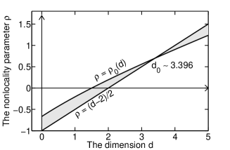
In the figure , where is the Lambert function.
For the MBE equation MBEDRG , we obtain . Interestingly, the one-loop DRG result MBEDRG , as well as the Self Consistent Expansion MBESCE yield , and so the inequality is saturated.
We could envisage, of course, systems that belong simultaneously to both classes. In such systems both inequalities (14) and (17) combine to give the equality . Reflecting about it, this is the case of model B. More precisely, we claim that although model B does not belong strictly to class II, it still effectively belongs to that class. The reason is that in model B the Hamiltonian can be replaced by obtained by setting in . Using puts the dynamical system in class II as well as in class I. Since the two Hamiltonians and are equivalent, at least, in the disordered phase, we conclude that for model B: . Thus the result of Ref. HH for model B using RG, seems to be exact. Note that the fact that they obtained this result to all orders in still may be consistent with (14) holding as a strict inequality. On the other hand, the proof we present here still depends strongly on a scaling assumption.
To summarize, in this paper we showed how to generalize the Schwartz-Soffer inequality derived originally for quenched random systems SS to dynamical stochastic systems. We show that the inequality, which involves the correlation and the response functions can be translated into a simple inequality relating the scaling exponents , , and the noise correlation exponent . It turns out that many physical dynamical systems discussed in the literature belong to one of two classes (or to both). In each of these classes there is a (different) additional relation. For class I, i.e. that of Hamiltonian systems, the additional relation is . For class II of Galilean invariant systems, the additional relation is . These two relations result in two complementary inequalities, for class I and for class II. For systems belonging to both classes we arrive at the conclusion that . We presented a number of cases where the inequality is rather tight or even saturated. We also show that in spite of being extremely simple, the inequality can be quite powerful when examining analytical, numerical and experimental results. To demonstrate the utility of the inequality from that aspect, we reviewed analytical results for the nonlocal KPZ model, by one method: the Dynamical Renormalization Group which is shown to disobey the inequality for a whole range of parameters. This has an important implication on the choice of analytical tools when dealing with such stochastic models.
It would be surprising if the two classes above cover all the possible dynamical systems. An open question remains if there exist other classes, involving stochastic driving, which are relevant in describing physical systems. Another open question is whether there are more systems of interest that belong to classes I and II simultaneously. Hopefully, the simplicity yet strength of this result will motivate researchers to explore the usefulness of rigorous inequalities and derive improved ones alongside the more popular chase of approximate equalities.
References
- (1) P.C. Hohenberg and B.I. Halperin, Rev. Mod. Phys. 49, 435 (1977).
- (2) M. Kardar, G. Parisi and Y.-C. Zhang, Phys. Rev. Lett. 56, 889 (1986).
- (3) S.F. Edwards and D. R. Wilkinson, Proc. R. Soc. London Ser. A 381, 17 (1982).
- (4) S. Mukherji and S. M. Bhattacharjee, Phys. Rev. Lett. 79, 2502 (1997).
- (5) A. Kr. Chattopadhyay, Phys. Rev. E 60, 293 (1999).
- (6) A.-L. Barabasi and H. E. Stanley, Fractal Concepts in Surface Growth (Cambridge Univ. Press, Cambridge, 1995).
- (7) R. Golestanian and E. Raphaël, Phys. Rev. E 67, 031603 (2003).
- (8) P. LeDoussal, K. J. Wiese, E. Raphaël and R. Golestanian, Phys. Rev. Lett. 96, 015702 (2006).
- (9) M. Adda-Bedia, E. Katzav and D. Vandembroucq, Phys. Rev. E 73, 035106(R) (2006); E. Katzav and M. Adda-Bedia, Europhys. Lett. 76, 450 (2006); E. Katzav et al., Phys. Rev. E 76, 051601 (2007).
- (10) E. Katzav, Physica A 309, 79 (2002).
- (11) E. Katzav, Physica A 308, 25 (2002).
- (12) E. Katzav, Phys. Rev. E 68, 031607 (2003).
- (13) R.A. da Silveira and M. Kardar, Phys. Rev. E 68, 046108 (2003).
- (14) M. Schwartz and A. Soffer, Phys. Rev. Lett. 55, 2499 (1985).
- (15) W.D. McComb, The Physics of Fluid Turbulence, O.U.P. Oxford (1990).
- (16) S.F. Edwards and M. Schwartz, Physica A 303, 357 (2002).
- (17) B.I. Halperin, P.C. Hohenberg and S.K Ma, Phys. Rev. Lett. 29 1548 (1972); Z. Racz and M.F. Collins, Phys. Rev. B 13, 3074 (1976); C. De Dominicis et al. Phys. Rev. B 15, 4313 (1977); M. Campellone and J.P. Bouchaud, J. Phys. A: Math. Gen. 30, 3333 (1997).
- (18) Z.-W. Lai and S. Das Sarma, Phys. Rev. Lett. 66, 2348 (1991).
- (19) J.P. Bouchaud and M.E. Cates, Phys. Rev. E 47, 1455(R) (1993).
- (20) J.P. Doherty et al., Phys. Rev. Lett. 72, 2041 (1994).
- (21) F. Colaiori and M.A. Moore, Phys. Rev. Lett. 86, 3946 (2001).
- (22) A. A. Fedorenko, Phys. Rev. B 77, 094203 (2008).
- (23) H. G. E. Hentschel and F. Family, Phys. Rev. Lett. 66, 1982 (1991).
- (24) M. Schwartz and S.F. Edwards, Europhys. Lett. 20, 301 (1992); Phys. Rev. E 57, 5730 (1998).
- (25) L. Canet et al., Phys. Rev. Lett. 104, 150601 (2010).
- (26) J. M. Kim and J. M. Kosterlitz, Phys. Rev. Lett. 62, 2289 (1989); L.-H. Tang, B. M. Forrest, and D. E. Wolf, Phys. Rev. A 45, 7162 (1992); C. S. Chin and M. den Nijs, Phys. Rev. E 59, 2633 (1999); E. Marinari, A. Pagnani, and G. Parisi, J. Phys. A 33, 8181 (2000); S. V. Ghaisas, Phys. Rev. E 73, 022601 (2006); V. G. Miranda and F. D. A. Aãrao Reis, Phys. Rev. E 77, 031134 (2008).
- (27) B. Hu and G. Tang, Phys. Rev. E 66, 026105 (2002).
- (28) G. Tang and B. Ma, Int. Jour. Mod. Phys. B 15, 2275 (2001); Physica A 298, 257 (2001).
- (29) E. Katzav and M. Schwartz, Europhys. Lett. 95, 66003 (2011).
- (30) E. Katzav and M. Schwartz, Phys. Rev. E 60, 5677 (1999).
- (31) E. Katzav, Phys. Rev. E 68, 046113 (2003).
- (32) E. Katzav, Phys. Rev. E 65, 32103 (2002).