Application of the dual-kinetic-balance sets in the relativistic many-body problem of atomic structure

Abstract

The dual-kinetic-balance (DKB) finite basis set method for solving the Dirac equation for hydrogen-like ions [V. M. Shabaev et al., Phys. Rev. Lett. 93, 130405 (2004)] is extended to problems with a non-local spherically-symmetric Dirac-Hartree-Fock potential. We implement the DKB method using B-spline basis sets and compare its performance with the widely-employed approach of Notre Dame (ND) group [W.R. Johnson and J. Sapirstein, Phys. Rev. Lett. 57, 1126 (1986)]. We compare the performance of the ND and DKB methods by computing various properties of Cs atom: energies, hyperfine integrals, the parity-non-conserving amplitude of the $6s_{1/2}-7s_{1/2}$ transition, and the second-order many-body correction to the removal energy of the valence electrons. We find that for a comparable size of the basis set the accuracy of both methods is similar for matrix elements accumulated far from the nuclear region. However, for atomic properties determined by small distances, the DKB method outperforms the ND approach. In addition, we present a strategy for optimizing the size of the basis sets by choosing progressively smaller number of basis functions for increasingly higher partial waves. This strategy exploits suppression of contributions of high partial waves to typical many-body correlation corrections.

I Introduction

Applications of perturbation theory in quantum mechanics require summations over a complete set of states of the lowest-order Hamiltonian. Usually, the relevant spectrum is innumerable. In practical applications such eigenspectra are often modeled using finite basis sets, chosen to be numerically complete. Since the sets are finite, the otherwise infinite summations become amendable to numerical evaluations.

The use of a finite basis set composed of piecewise polynomials, so-called B-splines de Boor (2001), has proven to be particularly advantageous in atomic physics and quantum chemistry applications Bachau et al. (2001). In this approach, an atom is placed in a sufficiently large cavity and the atomic wavefunctions are expanded in terms of the underlying B-spline set. Further, the variational Galerkin method is invoked and the solution of the resulting matrix eigenvalue problem produces a quasi-spectrum for the atom. In non-relativistic calculations, the lowest-energy orbitals of the resulting basis set closely agree with those of the unperturbed atom, and calculations of various properties of the low-lying states can be carried out. In particular, one could generate single-particle orbitals in some suitable lowest-order approximation, and use the resulting basis set in applications of many-body perturbation theory (MBPT) .

Application of the outlined approach to the relativistic problems brings in a complication– the appearance in the atomic quasi-spectrum of non-physical “spurious” states. These states appear in the solution of the single-particle radial Dirac equation for $\kappa>0$ angular symmetry, $j=\ell-1/2$ ( $p_{1/2},d_{3/2},\ldots$ orbitals). The spurious states rapidly oscillate and, moreover, spoil the mapping of the generated quasi-spectrum onto the low-energy orbitals of the atom. At the same time they are required for keeping the set complete. The problem of spurious states was discussed in the literature in details, see e.g., Ref. Goldman (1985); Quiney et al. (1987); Johnson et al. (1988); Igarashi (2006), and several solutions were proposed. In the pioneering applications of the B-splines in relativistic many-body problem by the Notre Dame group, Johnson et al. (1988) added an artificial potential spike centered at the origin to the Hamiltonian matrix. The overall effect was to shift the spurious states to higher energies thus restoring the low-energy mapping to the physical states. We will refer to the sets generated using this prescription as the Notre Dame (ND) sets. Another solution was to use “kinetically-balanced” sets Quiney et al. (1987), which related the small and the large components of the basis set functions via the Pauli approximation. Recently, an extension of this method was proposed in Ref. Shabaev et al. (2004). Here, due to additional relations between the small and large components, the negative (Dirac sea) and positive energy spectra are treated in a symmetric fashion. To emphasize this built-in symmetry, the authors refer to their method as the “dual-kinetic-balance” (DKB) approach. In both methods (by contrast to the ND prescription), the spurious states were shown to be completely eliminated from the quasi-spectrum.

Motivated by the success of the DKB method in computing properties of hydrogen-like ionsShabaev et al. (2004); Igarashi (2006), here we investigate the suitability of the DKB method in modeling the spectrum of the (non-local) Dirac-Hartree-Fock (DHF) potential. We compare the performance of the ND and DKB methods by computing various properties of Cs atom: single-particle energies, hyperfine integrals, and the parity-non-conserving amplitude of the $6s_{1/2}-7s_{1/2}$ transition. We find that for properties involving matrix elements accumulated near the nucleus, the DKB method outperforms the ND approach. Otherwise, if the electronic integrals are accumulated far from the nucleus, both methods produce results of a similar quality.

In addition, we investigate a possibility of using varying number of basis set functions for different angular symmetries. Summations over intermediate states in expressions of perturbation theory are carried out both over angular quantum numbers $\kappa$ and for fixed $\kappa$ over radial quantum numbers. Usually, as $|\kappa|$ (and $\ell$) increases, the correlation corrections due to higher partial waves become progressively smaller. Intuitively, one expects that for higher partial waves it would be sufficient to use smaller radial basis sets of lesser quality. This would reduce storage requirements for many-body calculations (for example, in implementing coupled-cluster formalism ) and would speed up numerical evaluations. While such an approach is common in quantum chemistry, see, e.g., Ref.Davidson and Feller (1986), the question of building the optimal B-spline basis set was not addressed yet in relativistic many-body calculations. We illustrate optimizing the basis sets by computing the second-order energy correction for several states of Cs.

This paper is organized as follows. First we recapitulate the Galerkin-type approach to generating a finite-basis set quasi-spectrum for the Dirac equation in Section II. The variational method is invoked for relativistic action and the problem is reduced to solving the generalized eigenvalue problem in Section II.1. The DHF potential is specified in Section II.2. Further we specify ND and DKB sets in Section II.3 and boundary conditions in Section II.4. A numerical analysis of Cs atom is provided in Section III. In Sections III.1 and III.2 we compare the performance of the ND and the DKB sets by computing single-particle energies, hyperfine integrals (Section III.1), and parity-nonconserving amplitudes (Section III.2) using both methods. The spurious states arising from the ND method are examined in Section III.3. In Section III.4 we consider second-order energy corrections in the DKB method and discuss a strategy of optimizing the size of the basis set.

II Problem setup

We are interested in solving the eigenvalue equation $H_{D}u\left(\mathbf{r}\right)=\varepsilon~{}u\left(\mathbf{r}\right)$ for the Dirac Hamiltonian, $H_{D}=c\mathbf{\alpha\cdot p}+\beta c^{2}+V_{\mathrm{nuc}}\left(r\right)+V_{\mathrm{DHF}}\left(r\right)$, where $V_{\mathrm{nuc}}$ is the nuclear potential and $V_{\mathrm{DHF}}$ is the mean-field (Dirac-Hartree-Fock) potential. $V_{\mathrm{DHF}}$ is in general a non-local potential. Assuming that both potentials are central one may exploit the rotational invariance to parameterize the solutions as

$$u_{n\kappa}(\mathbf{r})=\frac{1}{r}\left(\begin{array}[c]{c}iP_{n\kappa}(r)\ \Omega_{\kappa m}(\mathbf{\hat{r}})\\ Q_{n\kappa}(r)\ \Omega_{-\kappa m}(\mathbf{\hat{r}})\end{array}\right),$$ (1)

with $\Omega_{\kappa m}(\mathbf{\hat{r}})$ being the spherical spinors. The solutions depend on the radial quantum number $n$ and the angular quantum number $\kappa=(l-j)\left(2j+1\right)$. The large, $P_{n\kappa}$, and small, $Q_{n\kappa}$, radial components satisfy the conventional set of radial Dirac equations

$$\left(V_{\mathrm{nuc}}\left(r\right)+V_{\mathrm{DHF}}\left(r\right)+c^{2}\right)P_{n\kappa}\left(r\right)+c\left(\frac{d}{dr}-\frac{\kappa}{r}\right)Q_{n\kappa}\left(r\right) =\varepsilon_{n\kappa}P_{n\kappa}\left(r\right),$$

$$-c\left(\frac{d}{dr}+\frac{\kappa}{r}\right)P_{n\kappa}\left(r\right)+\left(V_{\mathrm{nuc}}\left(r\right)+V_{\mathrm{DHF}}\left(r\right)-c^{2}\right)Q_{n\kappa}\left(r\right) =\varepsilon_{n\kappa}Q_{n\kappa}\left(r\right).$$

These radial equations may be derived by seeking an extremum of the following action Johnson et al. (1988)

$$S = \frac{1}{2}c\int\left\{P\left(r\right)\hat{O}_{-}Q\left(r\right)-Q\left(r\right)\hat{O}_{+}P\left(r\right)\right\}dr+\frac{1}{2}\int\left(P\left(r\right),Q\left(r\right)\right)\hat{V}_{\mathrm{DHF}}\left(\begin{array}[c]{c}P\left(r\right)\\ Q\left(r\right)\end{array}\right)dr$$ (4)

$$+ \frac{1}{2}\int V_{\mathrm{nuc}}\left(r\right)\left(P\left(r\right)^{2}+Q\left(r\right)^{2}\right)dr-c^{2}\int Q\left(r\right)^{2}dr-\varepsilon\frac{1}{2}\int\left(P\left(r\right)^{2}+Q\left(r\right)^{2}\right)dr+\Delta S^{\mathrm{bnd}}+\Delta S^{\mathrm{spur}},$$ (5)

where the $\kappa$-dependent Pauli operators are defined as

$$\hat{O}_{\pm}^{\kappa}=\frac{d}{dr}\pm\frac{\kappa}{r}.$$

Radial integrals here and below have implicit limits from $r=0$ to $r=R$, where $R$ is the radius of the confining cavity. Boundary conditions may be imposed by adding the term $\Delta S^{\mathrm{bnd}}$ to the action. The term $\Delta S^{\mathrm{spur}}$ controls the appearance of the spurious states in the quasi-spectrum. We will specify these two terms below.

II.1 Reduction to the matrix form

We employ two finite basis sets $\left\{l_{i}\left(r\right)\right\}$ and $\left\{s_{i}\left(r\right)\right\},$ $i=\overline{1,2N}$, which, since we are interested in solving the (angularly-decoupled) radial equations, may depend on the angular quantum number $\kappa$. We may expand the large and small components in terms of these bases

$$P\left(r\right) = \sum_{i=1}^{2N}p_{i}~{}l_{i}\left(r\right),$$ (6)

$$Q\left(r\right) = \sum_{i=1}^{2N}p_{i}~{}s_{i}\left(r\right),$$

the expansion coefficients being the same for both the large and the small components. The above expansions are plugged into the action, Eq. (5), and, further, its extremum is sought by varying the expansion coefficients. As a result one arrives at the following generalized eigenvalue equation

$$A\vec{p}=\varepsilon B\vec{p},$$ (7)

where $A$ and $B$ are $2N\times 2N$ matrixes and $\vec{p}$ is the vector of expansion coefficients in Eq.(6). The matrix elements $A$ are given by

$$A_{ij}=D_{ij}+V_{ij}-2c^{2}S_{ij}+A_{ij}^{\mathrm{bnd}}+A_{ij}^{\mathrm{spur}}\,.$$ (8)

The matrixes entering the definition of $A$ correspond to various pieces of the radial Dirac equations,

$$D_{ij} =c\left(\int l_{i}\left(r\right)\frac{d}{dr}s_{j}\left(r\right)dr-\int l_{i}\left(r\right)\left(\frac{\kappa}{r}\right)s_{j}\left(r\right)dr\right)$$

$$+c\left(\int l_{j}\left(r\right)\frac{d}{dr}s_{i}\left(r\right)dr-\int l_{j}\left(r\right)\left(\frac{\kappa}{r}\right)s_{i}\left(r\right)dr\right),$$ (9)

$$V_{ij} =\int V_{\mathrm{nuc}}\left(r\right)\left[l_{i}\left(r\right)l_{j}\left(r\right)+s_{i}\left(r\right)s_{j}\left(r\right)\right]dr$$

$$+\left(V_{\mathrm{DHF}}\right)_{ij},$$ (10)

$$S_{ij} =\int s_{i}\left(r\right)s_{j}\left(r\right)dr,$$ (11)

with the matrix elements of the DHF potential, $\left(V_{\mathrm{DHF}}\right)_{ij}$, given below. The terms $A_{ij}^{\mathrm{bnd}}$ and $A_{ij}^{\mathrm{spur}}$ arise from the boundary and “spurious state” corrections in the action. Finally, the matrix $B$, $B_{ij}=\int\left[l_{i}\left(r\right)l_{j}\left(r\right)+s_{i}\left(r\right)s_{j}\left(r\right)\right]dr,$ reflects the fact that the basis sets may be non-orthonormal.

II.2 Potentials

The nuclear potential $V_{\mathrm{nuc}}\left(r\right)$ is generated for a nucleus of a finite size. We employ the Fermi distribution with the nuclear parameters taken from Ref. Johnson and Soff (1985). As to the Dirac-Hartree-Fock potential, we employ the frozen-core approximation. In this method, the calculation is carried out in two stages. First, the core orbitals are computed self-consistently. Second, based on the precomputed core orbitals, the DHF potential is assembled for the valence orbitals and the valence orbitals are determined. In the valence part of the problem, the core orbitals are no longer adjusted. Explicitly, for a set of the angular symmetry $\kappa$,

$$\left(V_{\mathrm{DHF}}\right)_{ij} =\int\left(\begin{array}[c]{cc}l_{i}&s_{i}\end{array}\right)\hat{V}_{\mathrm{DHF}}\left(\begin{tabular}[c]{l}$l_{j}$\\ $s_{j}$\end{tabular}\right)$$ (15)

$$=\left(V_{\mathrm{DHF}}^{\mathrm{dir}}\right)_{ij}+\left(V_{\mathrm{DHF}}^{\mathrm{exc}}\right)_{ij},$$ (16)

$$\left(V_{\mathrm{DHF}}^{\mathrm{dir}}\right)_{ij} =\sum_{a\in\mathrm{core}}\left(2j_{a}+1\right)$$

$$\times\int v_{0}\left(a,a,r\right)\left[l_{i}\left(r\right)l_{j}\left(r\right)+s_{i}\left(r\right)s_{j}\left(r\right)\right]dr,$$ (17)

$$\left(V_{\mathrm{DHF}}^{\mathrm{exc}}\right)_{ij} =-\sum_{a\in\mathrm{core}}\sum_{L}\left(2j_{a}+1\right)\Lambda_{\kappa L\kappa_{a}}$$

$$\times\int v_{L}\left(a,j,r\right)\left[l_{i}\left(r\right)P_{a}\left(r\right)+s_{i}\left(r\right)Q_{a}\left(r\right)\right]dr,$$ (18)

with the conventionally defined multipolar contributions

$$v_{L}\left(b,a,r\right)=\int\frac{r_{<}^{L}}{r_{>}^{L+1}}\left[P_{a}\left(r^{\prime}\right)P_{b}\left(r^{\prime}\right)+Q_{a}\left(r^{\prime}\right)Q_{b}\left(r^{\prime}\right)\right]dr^{\prime},$$ (19)

and the angular coefficient

$$\Lambda_{\kappa_{a}L\kappa_{b}}=\left(\begin{array}[c]{ccc}j_{a}&j_{b}&L\\ -1/2&1/2&0\end{array}\right)^{2}.$$ (20)

II.3 ND and DKB sets

Now we specify the Notre Dame (ND) and the dual-kinetic-balance (DKB) basis sets. Both operate in terms of B-spline functions and first we recapitulate the relevant properties of these splines. A set of $n$ B-splines of order $k$ is defined on a supporting grid $\left\{t_{i}\right\},i=\overline{1,n+k}$. Usually, the gridpoints are chosen as

$$t_{1} =t_{2}=\cdots=t_{k}=0,$$

$$t_{n} =t_{n+1}=\cdots=t_{n+k}=R.$$

In our calculations the intermediate gridpoints are distributed exponentially. B-spline number $i$ of order $k\,$, $B_{i}^{\left(k\right)}\left(r\right)$, is a piecewise polynomial of degree $k-1$ inside $t_{i}\leq r\ <t_{i+k}$. It vanishes outside this interval. This property simplifies the evaluation of matrix elements between the functions of the basis set. In addition, we will make use of the fact that as $r\rightarrow 0$, the first $k$ splines behave as (all the remaining splines are zero)

$$B_{i\leq k}^{\left(k\right)}\propto r^{i-1},$$ (21)

and at $r=R$, all splines vanish except for the last spline, $B_{i=n}^{\left(k\right)}$.

The Notre Dame set is defined as

$$l_{i}^{\mathrm{ND}}\left(r\right) =\left\{\begin{array}[c]{cc}B_{i}^{\left(k\right)}\left(r\right)&1\leq i\leq n\\ 0&n<i\leq 2n\end{array}\right.,$$ (24)

$$s_{i}^{\mathrm{ND}}\left(r\right) =\left\{\begin{array}[c]{cc}0&1\leq i\leq n\\ B_{i-n}^{\left(k\right)}\left(r\right)&n<i\leq 2n\end{array}\right..$$ (27)

It corresponds to an independent expansion of the large and small radial components into the B-spline basis. The DKB set involves the Pauli operators and enforces a “kinetic balance” between contributions to the components:

$$l_{i}^{\mathrm{DKB}}\left(r\right) =\left\{\begin{array}[c]{cc}-B_{i}^{\left(k\right)}\left(r\right)&1\leq i\leq n\\ -\frac{1}{2c}\hat{O}_{-}^{\kappa}~{}B_{i-n}^{\left(k\right)}\left(r\right)&n<i\leq 2n\end{array}\right.,$$ (30)

$$s_{i}^{\mathrm{DKB}}\left(r\right) =\left\{\begin{array}[c]{cc}\frac{1}{2c}\hat{O}_{+}^{\kappa}~{}B_{i}^{\left(k\right)}\left(r\right)&1\leq i\leq n\\ B_{i-n}^{\left(k\right)}\left(r\right)&n<i\leq 2n\end{array}\right..$$ (33)

Notice that, as discussed below, to satisfy the boundary conditions, we will use only a subset of the entire DKB basis.

II.4 Spurious states and boundary conditions

With the ND set, the spurious states are shifted away to the high-energy end of the quasi-spectrum by adding the following action Johnson et al. (1988) $\left(\Delta S^{\mathrm{spur}}\right)_{\mathrm{ND}}=\frac{c}{2}P\left(0\right)^{2}-\frac{c}{2}P\left(0\right)Q\left(0\right)$ for $\kappa<0$ and $\left(\Delta S^{\mathrm{spur}}\right)_{\mathrm{ND}}=c^{2}P\left(0\right)^{2}-\frac{c}{2}P\left(0\right)Q\left(0\right)$ for $\kappa>0$. This correction may be seen as arising from an artificial $\delta-$function-like potential centered at the origin. Unfortunately, as shown below in numerical examples, this additional spike perturbs the behavior of the orbitals near the nucleus. (As discussed below $\left(\Delta S^{\mathrm{spur}}\right)_{\mathrm{ND}}$ also sets the boundary conditions at $r=0.$) The DKB set does not have the spurious states at all, so that $\left(\Delta S^{\mathrm{spur}}\right)_{\mathrm{DKB}}\equiv 0$.

We need to specify boundary conditions at $r=0$ and at the cavity radius, $r=R$. We start by discussing the boundary conditions at $r=0$. For a finite-size nucleus the radial components behave as

$$P_{n\kappa} \propto r^{l+1}~{}\mathrm{and}~{}Q_{n\kappa}\propto r^{l+2}~{}\mathrm{for~{}}\kappa<0~{},$$ (34)

$$P_{n\kappa} \propto r^{l+1}~{}\mathrm{and}~{}Q_{n\kappa}\propto r^{l}~{}~{}~{}~{}\mathrm{for~{}}\kappa>0~{}.$$

In the Notre Dame approach, the boundary conditions are imposed variationally by adding the boundary terms to the action integral. Varying $\Delta S^{\mathrm{spur}}$, Ref.Johnson et al. (1988), effectively reduces to $P\left(0\right)=0$. In practice, because of the variational nature of the ND constraint, the large component, although being small, does not vanish at the origin, and the limits, (34), are not satisfied. Alternatively, Froese-Fischer and Parpia (1993) proposed to impose $P\left(0\right)=Q(0)=0$ by discarding the first B-spline of the set (this is the only B-spline that does not vanish at $r=0$). This is a “hard” constraint, since the wavefunction, Eq.(6), would vanish identically at the origin. In our calculations, because of our motivation in building the smallest possible basis set, we extend this scheme further. We exploit the power-law behavior of the B-splines, Eq.(21), and match it to the small-$r$ limits (34). To satisfy the matching, we need to include the B-splines starting with the sequential number ($i_{\min}$ must be smaller than the order of the splines $k$).

$$i_{\min}=|\kappa|+1=\left\{\begin{array}[c]{cc}\ell+2,&\kappa<0\\ \ell+1,&\kappa>0\end{array}\right..$$ (35)

For $s_{1/2}\left(\kappa=-1\right)\,$ and $p_{1/2}\left(\kappa=+1\right),\,i_{\min}=2,$ and this is equivalent to the boundary condition of Ref. Froese-Fischer and Parpia (1993). For higher partial waves, however, an increasingly larger number of splines is discarded: e.g., for $f_{7/2}\left(\kappa=-4\right),~{}i_{\min}=5$. One should notice that for a basis that includes partial waves  $\ell\leq\ell_{\max}$, for a faithful representation of the small-$r$ behavior in all the partial waves, one needs to require the order of the splines to be at least of $k=\ell_{\max}+3$. In particular, for $k=7$, $l_{\max}=4$.

When the first B-spline of the set, $B_{i=1}^{\left(k\right)}\left(r\right)$, is included in the basis (as in the ND approach), there is another difficulty in the calculations: since it’s value does not vanish at $r=0$, the matrix elements $D_{1,n+1}$ and $D_{n+1,1}$, which contain matrix elements of $1/r$, are infinite in absolute value Igarashi (2006). In practical calculations, one uses Gaussian quadratures to evaluate this integral, so the result of the integration is finite. Yet this introduces arbitrariness in the ND calculations and may be a reason for a relatively poor representation of the orbitals near the origin.

At the cavity radius, to avoid overspecifying the boundary conditions for the Dirac equation, the ND group used the boundary condition $P\left(R\right)=Q\left(R\right)$. As with the conditions at the origin, this relation was “encouraged”variationally. In our calculations (similarly to Ref. Shabaev et al. (2004)) we use the “hard” condition $P\left(R\right)=Q\left(R\right)=0$ by removing the last B-spline from the set. Examination of the resulting orbitals reveals that the wavefunctions acquire a non-physical inflection towards the end of the supporting grid, while the ND orbitals behave properly. Further numerical experimentation, however, shows that the inflection does not degrade the numerical quality at least for the atomic properties of the low-lying bound states of interest. At the same time, throwing away the last B-spline reduces the number of basis functions and leads to a more compact set.

To summarize, we will use the DKB basis set that includes B-splines with sequential numbers $i_{\mathrm{min}}(\kappa)$, Eq. (35) to $i_{\mathrm{max}}=n-1$. We will simply refer to this choice as the DKB basis. When we refer to $N=40$ DKB functions for a given partial wave, it would imply larger underlying B-spline set, e.g., for $s$-waves the total number of B-splines would be $n=42$. For the ND basis $n=N$, as all B-splines participate in the expansion.

In the remainder of this paper we present results of numerical analysis for ¹³³Cs atom. It is an atom with a single valence electron outside a closed-shell core. As the first step we carry out finite-difference Dirac-Hartree-Fock calculations for Cs core. The core orbitals are fed into the spline code where they are used to compute the matrix elements of the $V_{\mathrm{DHF}}$ potential, Eq.(16). As in Ref. Johnson et al. (1988) the numerical accuracy is monitored by comparing the resulting quasi-spectrum with the DHF energies from the finite-difference code.

III Numerical examples for Cs atom

Here we provide numerical examples involving both ND and DKB sets for Cs atom. In the two Sections immediately following we compare the performance of the ND and the DKB sets. We generate the quasi-spectrum using both ND and DKB sets and carry out comparisons for single-particle energies and hyperfine integrals in Section III.1 and parity-nonconserving amplitude in Section III.2. Section III.3 contains an analysis of spurious states in the ND method. In Section III.4 we analyze second-order energy corrections and discuss a strategy of optimizing the size of the basis.

III.1 Energies and hyperfine integrals

We compare ND and DKB quasi-spectrums with energies obtained using a finite-difference DHF code for the low-lying valence states in Table 1. The ND and DKB calculations were carried out using $N=40$ basis functions for B-splines of order $k=7$. We used a cavity of radius $R=50$ bohr. For the cavity of this size, only a few lowest-energy orbitals remain relatively unperturbed by the cavity. From examining Table 1, it is clear that both ND and DKB sets have a similar accuracy for energies.

In the second part of Table 1 we compare values of the radial integrals entering matrix elements of the hyperfine interaction due to the electric (EJ) and magnetic (MJ) multipolar moments of a point-like nucleus

$$I_{EJ}\left(n\kappa\right) =\int\frac{dr}{r^{J+1}}\left(P_{n\kappa}^{2}\left(r\right)+Q_{n\kappa}^{2}\left(r\right)\right),$$

$$I_{MJ}\left(n\kappa\right) =2\int\frac{dr}{r^{J+1}}P_{n\kappa}\left(r\right)Q_{n\kappa}\left(r\right).$$

The angular selection rules require $j\leq J/2$. We use identical integration grid for all three cases (DHF,ND,DKB) listed in the Table. The grid is sufficiently dense near the origin, it contains about 100 points inside the nucleus. The numerical integration excludes the first interval of the grid. From examining the Table we find that the DKB set outperforms the ND basis. While the ND set still recovers two-three significant figures for the magnetic-dipole coupling, it produces wrong results for electric-quadrupole and magnetic-octupole integrals. Certainly, the accuracy in the ND case improves for a larger basis set, but larger basis sets come at an additional computational cost. We carried out similar comparisons for matrix elements of the electric-dipole operator. As for the energies, we find that both the ND and DKB sets perform with a similar numerical accuracy.

As we have mentioned, $\left(\Delta S^{\mathrm{spur}}\right)_{\mathrm{ND}}$ variationally encourages the boundary condition $P\left(0\right)=0$. However, there is no such explicit encouragement for $Q\left(0\right)$. Here we qualitatively discuss the observed properties of the radial components near the origin for the Cs ND set. We see that, though their general behavior is to approach zero, the large component wavefunctions often have small improper inflections or oscillations near the origin. Small component wavefunctions, on the other hand, often do not even approach zero. These improper behaviors seem to be exemplified as we look at states higher in the spectrum. As we have seen here, such improper behavior of both the large and small component radial functions near the origin prove detrimental for properties accumulated near the nucleus. We conclude that while producing the results of a similar quality for matrix elements accumulated far from $r=0$, the DKB set provides a better approximation to the atomic orbitals near the nucleus.

State	Set	Energy	M1 HFI	E2 HFI	M3 HFI
$6s_{1/2}$	FD	$-0.1273680$	$1.114751[-1]$
	DKB	$-0.1273674$	$1.114741[-1]$
	ND	$-0.1273682$	$1.121812[-1]$
$7s_{1/2}$	FD	$-0.5518735[-1]$	$3.063077[-2]$
	DKB	$-0.5518714[-1]$	$3.063069[-2]$
	ND	$-0.5518750[-1]$	$3.084164[-2]$
$6p_{1/2}$	FD	$-0.8561589[-1]$	$-1.252026[-2]$
	DKB	$-0.8561576[-1]$	$-1.252018[-2]$
	ND	$-0.8561616[-1]$	$-1.218362[-2]$
$6p_{3/2}$	FD	$-0.8378548[-1]$	$4.649107[-3]$	$6.693978[-1]$	$8.725496[0]$
	DKB	$-0.8378543[-1]$	$4.649117[-3]$	$6.694037[-1]$	$8.744759[0]$
	ND	$-0.8378538[-1]$	$4.649454[-3]$	$1.591405[+2]$	$1.924786[7]$
$5d_{3/2}$	FD	$-0.6441964[-1]$	$-3.543808[-3]$	$1.702467[-1]$	$-8.950592[1]$
	DKB	$-0.6441961[-1]$	$-3.543799[-3]$	$1.702736[-1]$	$-9.202786[1]$
	ND	$-0.6441970[-1]$	$-3.038702[-3]$	$1.643100[+5]$	$3.663198[10]$
$5d_{5/2}$	FD	$-0.6452977[-1]$	$2.257618[-3]$	$1.562954[-1]$	$1.938370[1]$
	DKB	$-0.6452976[-1]$	$2.257616[-3]$	$1.562953[-1]$	$1.938705[1]$
	ND	$-0.6452969[-1]$	$2.257607[-3]$	$7.144243[+0]$	$7.235873[5]$

Table 1: Comparison of the energies and radial integrals of the hyperfine interaction in the Dirac-Hartree-Fock approximation for Cs. FD marks values produced by a finite-difference code. DKB and ND values are generated with dual-kinetic-balance and Notre Dame B-spline basis sets. In both cases we used $N=40$ basis functions for B-splines of order $k=7$ in a cavity of $R=50$ bohr. Notation $x[y]$ stands for $x\times 10^{y}$.

III.2 Parity-nonconserving amplitude

So far we examined properties of the individual basis set orbitals with sufficiently low energies. The real power of the finite basis set technique lies in approximating the entire innumerable spectrum by a finite size quasi-spectrum. This is important, for example, in computing sums over intermediate states (Green’s functions) in perturbation theory.

From the discussion of the preceding Section it is clear that the difference in quality of the ND and DKB basis sets is expected to become most apparent for the properties accumulated near the nucleus. Here, as an illustrative example, we consider the parity-nonconserving (PNC) amplitude for the $6S_{1/2}\rightarrow 7S_{1/2}$ transition in ${}^{133}\mathrm{Cs}$. This amplitude appears in the second order of perturbation theory for the otherwise forbidden dipole transition and it can be represented as a sum over intermediate states $np_{1/2}$

$$E_{\mathrm{PNC}} = \sum_{n=2}\frac{\langle 7s_{1/2}|D|np_{1/2}\rangle\langle np_{1/2}|H_{W}|6s_{1/2}\rangle}{\varepsilon_{6s_{1/2}}-\varepsilon_{np_{1/2}}}$$ (36)

$$+ \sum_{n=2}\frac{\langle 7s_{1/2}|H_{W}|np_{1/2}\rangle\langle np_{1/2}|D|6s_{1/2}\rangle}{\varepsilon_{6s_{1/2}}-\varepsilon_{np_{1/2}}}\,.~{}~{}$$

Here $D$ and $H_{\rm W}$ are electric-dipole and weak interaction (pseudo-scalar) operators, and $\varepsilon_{i}$ are atomic energy levels. We will compute this expression in the single-particle approximation. Specifically, the index $n$ runs over the entire DHF quasi-spectrum for $p_{1/2}$ partial wave, including core orbitals. The weak Hamiltonian reads

$$H_{\rm W}=\frac{G_{F}}{\sqrt{8}}Q_{\rm W}\rho_{\mathrm{n}uc}(r)\gamma_{5}\,,$$ (37)

where $G_{F}$ is the Fermi constant, $Q_{\rm W}$ is the weak charge, $\gamma_{5}$ is the Dirac matrix (it mixes large and small components), and $\rho_{\mathrm{n}uc}(r)$ is the neutron density distribution. For consistency with the previous calculations the $\rho_{\mathrm{n}uc}(r)$ is taken to be the proton Fermi distribution of Ref. Blundell et al. (1992). Notice that the matrix elements of the weak interaction are accumulated entirely inside the nucleus.

We evaluate the sum (36) using the DKB and the ND sets with $N=40$ basis functions of order $k=7$. The integration grids are the same in both cases and include large number of points ($\sim 100$) inside the nucleus. The PNC amplitude is conventionally expressed in units of $10^{-11}i|e|a_{0}(-Q_{\rm W}/N_{n})$, where $N_{n}=78$ is the number of neutrons in the nucleus of ¹³³Cs. In these units, the results are

$$E_{\mathrm{PNC}}^{\mathrm{FD}} = -0.740,$$

$$E_{\mathrm{PNC}}^{\mathrm{DKB}} = -0.7395\,(N=40,k=7),$$

$$E_{\mathrm{PNC}}^{\mathrm{ND}} = -0.8546\,(N=40,k=7).\,$$

The finite-difference value is taken from Ref. Blundell et al. (1992). Again we note that the DKB set offers an improved performance over the Notre Dame set. Reaching the comparable accuracy in the ND approximation requires a larger basis set. For example, $N=75,k=9$ ND set reproduces the DKB result for the PNC amplitude.

Further insights may be gained from examining individual contributions of the intermediate states in the PNC amplitude. We plot individual contributions of the intermediate state $np_{1/2}$ to the PNC amplitude in Fig. 1. Both terms in Eq.(36) are included. We computed the data using $N=100,k=11$ ND and DKB basis sets generated in a cavity of $R=50$ bohr. From the plot, we observe that the dominant contribution arises from the low-lying valence states. As $n$ increases, the contributions become quickly suppressed (there is 10 orders of magnitude suppression for $n\approx 50$). This is due to both increased energy denominators and decreased density at the nucleus for high $n$. Comparison between the basis sets reveals that their contributions are identical until $n=17$. For higher principal quantum numbers, the DKB contributions monotonically decrease, while ND contributions become irregular. Moreover, at $n=28$ the ND contributions start to flip signs with increasing $n$. Generally, this oscillating pattern would lead to a deterioration of the numerical accuracy. We believe that the described irregularity is again due to the aforementioned improper behavior of orbitals near the nucleus, as the matrix elements of the weak Hamiltonian is accumulated largely in this regime.

To summarize, the DKB set is numerically complete and is well suited for carrying out practical summations over intermediate states in perturbation theory. The comparison with the ND set shows that, at least for the PNC amplitude, the ND convergence pattern becomes affected by the inaccurate representation of the orbitals near the nucleus (this is exemplified for states higher in the spectrum), while the DKB set exhibits a monotonic convergence. Additionally, the DKB set is devoid of spurious states, and therefore the incidental inclusion of spurious states in summations over intermediate states is of no concern.

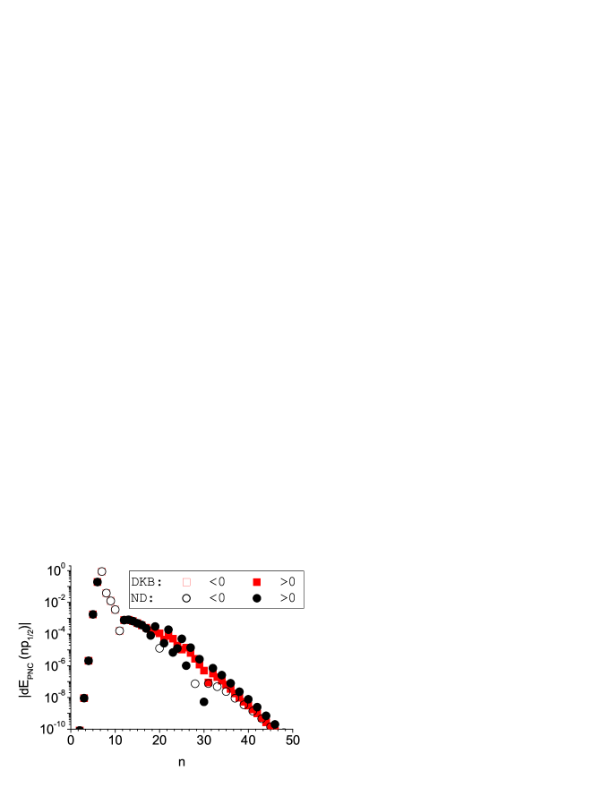
Figure 1: (Color online) Individual contributions of the $p_{1/2}$ intermediate states to the PNC amplitude, Eq.(36), as a function of the principal quantum number $n$. The units of the PNC amplitude are $10^{-11}i|e|a_{0}(-Q_{\rm W}/N_{n})$. The results from the DKB basis are represented by squares and those from the ND basis by circles. Both sets contain $N=100$ basis orbitals and use identical integration grids. Due to the employed logarithmic scale, we plot the absolute values of the contributions. We use hollow symbols to indicate negative contributions and filled symbols for marking positive contributions.

III.3 Analysis of spurious states in the ND method

Here we analyze the effect that the additional term $\left(\Delta S^{\mathrm{spur}}\right)_{\mathrm{ND}}$ has on spurious states which occur in the ND method. We start by taking

$$\Delta S^{\mathrm{spur}}=\left\{\begin{array}[c]{cc}x\frac{c}{2}P\left(0\right)^{2}-\frac{c}{2}P\left(0\right)Q\left(0\right),&\kappa<0\\ xc^{2}P\left(0\right)^{2}-\frac{c}{2}P\left(0\right)Q\left(0\right),&\kappa>0\\ \end{array}\right.,$$ (38)

with $x$ an adjustable parameter. For the case of $x=1$ this is equivalent to $\left(\Delta S^{\mathrm{spur}}\right)_{\mathrm{ND}}$. We mentioned previously that $\left(\Delta S^{\mathrm{spur}}\right)_{\mathrm{ND}}$ variationally encourages the boundary condition $P\left(0\right)=0$; this is also true for any choice of $x$. The specific choice of $x$ effectively alters the degree of such variational “encouragement.”

We find that setting $x=0$ results in a single spurious state which appears as the lowest energy eigenstate for each $\kappa>0$. By subsequently increasing the value of $x$ towards $x=1$ we may then deduce the effect that $\left(\Delta S^{\mathrm{spur}}\right)_{\mathrm{ND}}$ has on these spurious states as well as the rest of the spectrum. We find that small increases in $x$ from $x=0$ causes the energy of the spurious state to increase, while the other states remain essentially unaffected (except for the case of near degeneracy with one of these states; this situation is discussed below). As $x$ is increased from zero, we may watch as spurious states for each $\kappa>0$ first appear as the lowest energy state, then move up to the second lowest energy state, then to the third lowest energy state, etcetera. Fig. 2 displays this effect for the case of Cs.

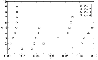
Figure 2: Location of the spurious state in the spectrum of Cs for $1\leq\kappa\leq 4$ at various values of $x$. Here $s$ corresponds to the location of the spurious state in the spectrum (e.g., $s=2$ corresponds to the spurious state appearing as the second lowest energy state for that $\kappa$). We used a set with $N=40$ B-splines of order $k=7$ confined to a cavity of radius $R=50$ bohr.

It is also interesting to analyze the effect of the spurious state when its energy is nearly degenerate with another state in the spectrum (we will refer to this other state as the “genuine” state). As the energies approach degeneracy by varying $x$, we observe that the spurious state begins to mix in with the genuine state. The first evidence for this is that the energy of the genuine state starts to become affected by the presence of the spurious state. Secondly, we see that the radial wavefunctions $P(r)$ and $Q(r)$ of the genuine state begin to acquire non-physical “bumps” that oscillate in a way that corresponds to the rapid oscillations of the respective spurious state radial functions. As the energy becomes nearly degenerate, the two states mix to such a degree that it is not even possible to define one as the “genuine state” and the other as the “spurious state.” This effect is shown in Fig. 3, where the genuine state is taken as the 4$d_{3/2}$ state of Cs. As $x$ is increased such that the spurious state becomes embedded in the quasi-continuum part of the spectrum, it mixes with multiple neighboring states, and at this point it becomes difficult to track or even define the spurious state.

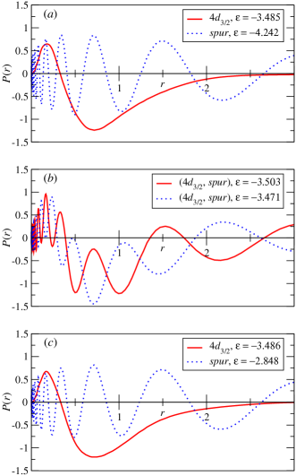
Figure 3: (Color online) Behavior of the large component radial wavefunction $P(r)$ of the $4d_{3/2}$ ($\kappa=2$) state of Cs when the spurious state is ($a$) just below it in the spectrum ($x=0.052$), ($b$) nearly degenerate with it ($x=0.054$), and ($c$) just above it in the spectrum ($x=0.056$). For the case ($b$), the notation $(4d_{3/2},spur)$ is used to indicate that the states are some linear combination of the two states and not easily defined as one or the other. Here $\varepsilon$ refers to the energy in a.u. with rest energy subtracted off. For reference, the ND set ($x=1$) gives the lowest three $d_{3/2}$ states to have energies: $3d_{3/2}$, $\varepsilon=-28.310$; $4d_{3/2}$, $\varepsilon=-3.486$; $5d_{3/2}$, $\varepsilon=-0.064$. We used a set with $N=40$ B-splines of order $k=7$ confined to a cavity of $R=50$ bohr; note that these plots only extend to $r=3$ bohr, however.

Presumably increasing $x$ to $x=1$ (the Notre Dame case) shifts the spurious states all the way to the end of the spectrum. Evidence for this is seen, for example, in the $d_{3/2}$ set used for Fig. 3 ($N=40$, $k=7$, $R=50$ bohr). Here the last few levels (excluding the very last level) have an energy spacing on the order of $10^{6}$ a.u., whereas the energy spacing to the final level is on the order of $10^{9}$ a.u. Furthermore, increasing $x$ past $x=1$ only has a substantial effect on the energy of the final level (for $x=10,000$ the energy spacing to the final level is then on the order of $10^{13}$ a.u.).

Up to this point we have been exclusively considering cases with $\kappa>0$, as these have been the only angular symmetries for which spurious states have previously been known to occur. Now we shall consider the effect that $\left(\Delta S^{\mathrm{spur}}\right)_{\mathrm{ND}}$ has on the cases of $\kappa<0$. As with the $\kappa>0$ cases, we see that increasing $x$ past $x=1$ only has a substantial effect on the energy of the final level. This is an indication that a spurious state may actually lie at the end of the spectrum for $\kappa<0$ angular symmetries as well. In fact, we find that setting $x$ to a negative value significantly below $x=0$ results in a single spurious state which appears as the lowest energy eigenstate for each $\kappa<0$. By subsequently increasing $x$ from this point, we may watch as each spurious state is shifted towards the higher energy end of the spectrum, similar to what is observed with $\kappa>0$ spurious states.

Now we return briefly to subject of the matrix elements $D_{1,n+1}$ and $D_{n+1,1}$ of the ND basis, which are suspected to contribute to poor representation of orbitals near the nucleus. From Eqs. (9) and (24) we see that these include the integral $\int\frac{1}{r}\left[B_{i=1}^{\left(k\right)}\left(r\right)\right]^{2}dr$, which is infinite due to the non-vanishing property of the first B-spline at $r=0$. Numerically this integral is evaluated by Gaussian quadrature, producing finite values. We observe that for the ($N=40$, $k=7$, $R=50$ bohr) Cs set, increasing the numerical value of this integral to 20 times its Gaussian quadrature value results in the reappearance of spurious states as the lowest energy eigenstates for each $\kappa>0$. Simultaneously, the energy of highest energy eigenstate for each $\kappa<0$ is increased substantially. Evidently the capability of $\left(\Delta S^{\mathrm{spur}}\right)_{\mathrm{ND}}$ to shift the spurious state to the end of the spectrum for $\kappa>0$ angular symmetries is reliant upon the inaccurate numerical evaluation of this (theoretically) infinite-value integral.

The claim made in this section of observing spurious states for $\kappa<0$ angular symmetries may seem surprising at first. Shabaev et al. (2004) have proved that an independent expansion of large and small radial components with a finite set of basis functions leads to a single spurious state for $\kappa>0$ angular symmetries. This proof assumes the basis functions to vanish at the origin, and the result of this proof is consistent with experience when such basis functions are employed. Arguably, connection is lost immediately with this proof because the ND set includes the first B-spline, which does not vanish at the origin. As we have seen here, the ND method depends on numerical inaccuracies in evaluating infinite-value integrals in order to manipulate spurious states arising in $\kappa>0$ cases. Because the ND method also includes the first B-spline for $\kappa<0$ angular symmetries (and hence similar numerical inaccuracies), we would have no reason to discount the possibility of spurious states from occurring in these cases as well.

III.4 Optimizing the basis set: second-order energy correction

In the preceding sections we established that the DKB sets are more robust than the ND bases. For a comparable size of the basis set the DKB basis exhibits better numerical accuracy for properties accumulated at small radii. Or, we may say that for a fixed numerical accuracy, the DKB basis may contain smaller number of basis functions. In this section we investigate a related question: what the smallest possible basis set is for a given numerical accuracy. Keeping the set as small as possible speeds up many-body calculations that usually require multiple summations over intermediate states. Also, smaller basis sets reduce storage requirements for expansion coefficients in all-order techniques such as configuration interaction or coupled-cluster methods.

Quantifying the numerical accuracy requires choosing some metric, which characterizes deviation of the selected property for a given basis from its exact value. Apparently, one should select the “metric” so that it can be easily computed and is related to the relevant atomic properties. As an example of an optimization measure, here we choose the second-order correction to the energy of a valence electron, $E_{v}^{\left(2\right)}$.

In the frozen-core DHF approximation $E_{v}^{\left(2\right)}$ is the leading many-body correction to the energy. It is given in terms of the Coulomb integrals $g_{ijkl}=\int d1d2u_{i}^{\dagger}(1)u_{j}^{\dagger}(2)\left(1/r_{12}\right)u_{k}(1)u_{l}(2)$ and single particle energies $\varepsilon_{i}$ as (see, e.g., Ref. Johnson (2007)) ,

$$E_{v}^{\left(2\right)}=\sum_{abn}\frac{\tilde{g}_{abvn}g_{vnab}}{\varepsilon_{v}+\varepsilon_{n}-\varepsilon_{a}-\varepsilon_{b}}-\sum_{mna}\frac{\tilde{g}_{vamn}g_{mnva}}{\varepsilon_{m}+\varepsilon_{n}-\varepsilon_{v}-\varepsilon_{a}}\,,$$ (39)

where $\tilde{g}_{ijkl}={g}_{ijkl}-{g}_{ijlk}$ is the antisymmetrized Coulomb integral. The summations are carried out over core orbitals (labels $a$ and $b$) and virtual (non-core) orbitals (labels $m$ and $n$). Each summation implies summing over principal quantum numbers, angular numbers $\kappa$, and magnetic quantum numbers. The summation over magnetic quantum numbers may be carried out analytically and we are left with summations over radial functions.

We define a contribution of an individual partial wave $\ell$, $\delta E^{(2)}_{v}(\ell)$, as the difference $\delta E^{(2)}_{v}(\ell)=E^{(2)}_{v}(\ell)-E^{(2)}_{v}(\ell-1)$, where $E^{(2)}_{v}(\ell)$ stands for truncated Eq. (39); it includes summations over intermediate states (both core and virtual) with the orbital angular momentum up to $\ell$. Since the calculations necessarily involve Coulomb integrals between orbitals of different angular momenta, the numerical error in $\delta E^{(2)}_{v}(\ell)$ is affected by the accuracy of representation of all partial waves up to $\ell$.

First, in Table 2, we present results for a large set of $N=100$ basis functions for each partial wave. We use a sufficiently large cavity of $R=50$ bohr in this calculation. These results will serve as a benchmark for comparisons with the less complete (optimized) sets. We observe that the dominant (60%) contribution comes from $d$-waves, $\ell=2$. Qualitatively, the second-order energy correction may be described as core-polarization effect. The outer $3d$-orbitals of the core are relatively “soft” and are easily polarizable. Since the core does not contain $f$ and higher partial waves, after peaking at $\ell=2$, the partial-wave contributions become suppressed as $\ell$ increases. Qualitatively, this suppression arises due to increased centrifugal repulsion of higher partial waves and associated smaller overlaps with core orbitals in the Coulomb integrals of Eq. (39). For example, $\ell=6$ contributes only 0.6% of the total value.

Now we would like to minimize the size of the set by choosing a different number of radial basis functions $N_{\kappa}$ for different angular symmetries $\kappa$. To preserve a numerical balance between the fine-structure components (for example, this may be important while recovering non-relativistic limit) we keep the same number of functions for a given orbital angular momentum $\ell$, e.g., $N_{p_{1/2}}=N_{p_{3/2}}$.

In Table 2, we present an example of an optimized basis (marked as “Small set”). We also list resulting numerical errors for each partial wave by comparing $\delta E^{(2)}_{6s}(\ell)$ with the result from the “Large set” calculations. We see that while the basis-set error in higher partial waves is as large as 40%, this hardly makes any influence on the total value of the correlation energy, because of contributions of higher $\ell$ are suppressed. The total value of the correlation correction differs by about 1% from it’s saturated value. Considering that the correlation contribution to the energy is about 10% for the $6s$ state, the less complete set would introduce only 0.1% error for the total ionization energy.

So far we discussed the correlation energy correction for the $6s_{1/2}$ state. The optimized set remains sufficiently robust for other low-lying states as well. We have carried out a comparison similar to Table 2 for $6p_{1/2}$, $6p_{3/2}$, $5d_{3/2}$, and $5d_{5/2}$ states. In all these cases the difference between the total $E^{(2)}_{v}$ values computed with the“Large” and “Small” sets is about 0.5%. In practical calculations one is often required to reproduce a number of properties with the same set. The atomic properties may be quite dissimilar– like hyperfine-structure interactions accumulated near the nucleus and dipole matrix elements determined by the valence region. Apparently, one has to carry out a similar low-order MBPT analysis for the relevant quantities to verify the suitability of the optimized set.

From the computational point of view, using the optimized sets speeds up the numerical evaluations. In our illustrative example, the “Large set” contains $N_{t}=(1+2\times 6)\times 100=1300$ orbitals, while the “Small set” is about four times smaller ($N_{t}=285$ orbitals). The resulting speed-up is sizable: our computations of Eq. (39) for the $6s_{1/2}$ state ($\ell=6$) are about 14 times faster with the optimized set, as expected due to $N_{t}^{2}$ scaling of the number of contribution in the most computationally demanding second term of Eq.(39). Similar scaling should hold for storage of expansion coefficients in all-order methods, e.g., for storing triple excitations Derevianko and Porsev (2007) one expects $N_{t}^{3}$ scaling of the storage size. Usually higher partial waves produce larger number of angular channels and the scaling should be even steeper than $N_{t}^{3}$. Further speed-up in MBPT summations and reduction in storage size may be attained by skipping a few basis set functions at the upper end of the quasispectrum. Such additional truncation of the spectrum becomes apparent from Fig. 1, where contributions to the PNC amplitude for the upper three-quarters ($n\gtrsim 25$ out of $N=100$) of the quasi-spectrum affect the total value below $10^{-4}$ level of accuracy.

$\ell$	Large set		Small set		Error
	$(N,k)$	$\delta E^{(2)}_{6s}(\ell)$	$(N,k)$	$\delta E^{(2)}_{6s}(\ell)$
0	(100,11)	-0.0000130	(35,7)	-0.0000122	6%
1	(100,11)	-0.0020027	(35,7)	-0.0019936	0.5%
2	(100,11)	-0.0105623	(30,5)	-0.0105373	0.2%
3	(100,11)	-0.0039347	(25,4)	-0.0039095	0.6%
4	(100,11)	-0.0007563	(15,4)	-0.0007269	4%
5	(100,11)	-0.0002737	(10,4)	-0.0002272	20%
6	(100,11)	-0.0001182	(10,4)	-0.0000844	40%
Total		-0.0176609		-0.0174912	1%

Table 2: Contribution of individual partial waves $\ell$ to the second-order energy correction for the ground $6S_{1/2}$ state of Cs atom. We use the DKB basis set of $N$ basis functions constructed from a subset of B-splines of order $k$ (label $(N,k)$). Calculations are carried out in a cavity of $R=50$ bohr for two basis sets “Large” and “Small”. Numerical integration grids are identical for both sets. The column marked “Error” refers to a relative error in a given partial-wave contribution, $\delta E^{(2)}_{6s}(\ell)$, caused by switching from the “Large” to the “Small” basis set.

IV Conclusion

Calculations of certain atomic properties, such as parity-violating amplitudes, transition polarizabilities between hyperfine levels, and many-body corrections to hyperfine interactions require accurate representation of atomic orbitals at both small and intermediate electron-nucleus distances. Solving the many-body problem in high orders of perturbation theory additionally calls for an efficient representation in terms of the basis sets. The dual-kinetic-basis set is shown here to adequately meet both these demands.

Previously the DKB basis was applied to systems with a single electron in a Coulomb field, i.e., hydrogen-like ionsShabaev et al. (2004); Igarashi (2006). Here we extended the DKB method to many-electron systems by generating the single-particle quasi-spectrum of the Dirac-Hartree-Fock potential. Several numerical example for Cs atom were presented. We showed that the DKB method outperforms the widely-employed Notre Dame B-spline method Johnson et al. (1988) for problems involving matrix elements accumulated at small distances.

In addition, we presented a strategy for optimizing the size of the basis sets by choosing progressively smaller number of basis functions for increasingly higher partial waves. This strategy exploits suppression of contributions of high partial waves to typical many-body correlation corrections.

V Acknowledgments

We would like to thank Walter Johnson, Charlotte Froese-Fischer, and Vladimir Shabaev for discussions. The developed dual-kinetic-balance code for the Dirac-Hartree-Fock problem was partially based on codes by the Notre Dame group. This work was supported in part by the National Science Foundation.

References

- de Boor (2001) C. de Boor, A practical guide to splines (Springer-Verlag, New York, 2001), revised ed.
- Bachau et al. (2001) H. Bachau, E. Cormier, P. Decleva, J. E. Hansen, and F. Martin, Rep. Prog. Phys. 64, 1815 (2001).
- Goldman (1985) S. P. Goldman, Phys. Rev. A 31, 3541 (1985).
- Quiney et al. (1987) H. M. Quiney, I. P. Grant, and S. Wilson, Phys. Scr. 36, 460 (1987).
- Johnson et al. (1988) W. R. Johnson, S. A. Blundell, and J. Sapirstein, Phys. Rev. A 37, 307 (1988).
- Igarashi (2006) A. Igarashi, J. Phys. Soc. Jap. 75, 114301/1 (2006).
- Shabaev et al. (2004) V. M. Shabaev, I. I. Tupitsyn, V. A. Yerokhin, G. Plunien, and G. Soff, Phys. Rev. Lett. 93, 130405 (pages 4) (2004).
- Davidson and Feller (1986) E. Davidson and D. Feller, Chem. Rev. 86, 681 (1986).
- Johnson and Soff (1985) W. R. Johnson and G. Soff, At. Data and Nucl. Data Tables 33, 405 (1985).
- Froese-Fischer and Parpia (1993) C. Froese-Fischer and F. A. Parpia, Phys. Lett. 179, 198 (1993).
- Blundell et al. (1992) S. A. Blundell, J. Sapirstein, and W. R. Johnson, Phys. Rev. D 45, 1602 (1992).
- Johnson (2007) W. R. Johnson, Atomic Structure Theory: Lectures on Atomic Physics (Springer, New York, NY, 2007).
- Derevianko and Porsev (2007) A. Derevianko and S. G. Porsev, Eur. J. Phys. A (2007).