A New Determination of the High Redshift Type Ia Supernova Rates with the Hubble Space Telescope Advanced Camera for Surveys.

Abstract

We present a new measurement of the volumetric rate of Type Ia supernova up to a redshift of 1.7, using the Hubble Space Telescope (HST) GOODS data combined with an additional HST dataset covering the North GOODS field collected in 2004. We employ a novel technique that does not require spectroscopic data for identifying Type Ia supernovae (although spectroscopic measurements of redshifts are used for over half the sample); instead we employ a Bayesian approach using only photometric data to calculate the probability that an object is a Type Ia supernova. This Bayesian technique can easily be modified to incorporate improved priors on supernova properties, and it is well-suited for future high-statistics supernovae searches in which spectroscopic follow up of all candidates will be impractical. Here, the method is validated on both ground- and space-based supernova data having some spectroscopic follow up. We combine our volumetric rate measurements with low redshift supernova data, and fit to a number of possible models for the evolution of the Type Ia supernova rate as a function of redshift. The data do not distinguish between a flat rate at redshift $>$ 0.5 and a previously proposed model, in which the Type Ia rate peaks at redshift $\sim$ 1 due to a significant delay from star-formation to the supernova explosion. Except for the highest redshifts, where the signal to noise ratio is generally too low to apply this technique, this approach yields smaller or comparable uncertainties than previous work.

1 Introduction

The empirical evidence for the existence of dark energy came from observations of Type Ia supernovae (Riess et al., 1998; Perlmutter et al., 1999; for review, see Perlmutter and Schmidt, 2003), which are believed to arise from the thermonuclear explosion of a progenitor white dwarf after it approaches the Chandrasekhar mass limit (Chandrasekhar, 1931). However, the physics of Type Ia supernova production is not well understood. The two most plausible scenarios for the white dwarf to accrete the necessary mass are the single degenerate case, where the white dwarf is located in a binary system; and the double degenerate case, where two white dwarfs merge. The Type Ia supernova rate is correlated with the star formation history (SFH), and thus a measurement of the rate as a function of redshift helps constrain the possible type Ia progenitor models.

In addition to its importance for understanding Type Ia supernovae as astronomical objects, a good grasp of the Type Ia supernova rate to high redshifts is important for the next generation of proposed space-based supernova cosmology experiments, such as SNAP (Aldering et al., 2004). It is therefore of great practical interest to determine the rate of Type Ia supernovae at redshifts $>$ 1.

The subject of Type Ia supernova rates has been addressed by many authors in the past. Existing rate measurements have been mostly limited to redshift ranges $<$ 1: the results of Cappellaro et al. (1999), Hardin et al. (2000), Madgwick et al. (2003), and Blanc et al. (2004) measure the rates at redshifts $\leq$ $\sim$0.1; Neill et al. (2006), Tonry et al. (2003), and Pain et al. (2002), at intermediate redshifts of 0.47, 0.50, and 0.55, respectively; and Barris and Tonry (2006), up to a redshift of 0.75. The only published measurement of the rates at redshifts $>$ 1 is that of Dahlen et al. (2004), who analyzed the GOODS dataset.

There are several important differences that distinguish our work from that of Dahlen et al. (2004). First, we augment the GOODS sample with the HST data collected during the Spring-Summer 2004 high redshift supernova searches. Second, our methods of calculating the control time (the time during which a supernova search is potentially capable of finding supernova candidates) and the efficiency to identify a supernova are based on a detailed Monte Carlo simulation technique using a library of supernova templates. Third, we adopt a novel approach to typing supernovae, using photometric data and a Bayesian probability method described in Kuznetsova and Connolly (2007). The Bayesian technique is able to perform classification using only photometric data, and therefore does not require spectroscopic follow up. Optionally, photometric or spectroscopic redshifts can be used to improve the classification accuracy. Our initial requirements on potential supernova candidates are more stringent in terms of the number of points on the light curve and the signal to noise of those points than those of Dahlen et al. (2004); thus some of the candidates they identified will fail our cuts. However, we are able to reliably separate Type Ia supernova from other supernovae types based on their Bayesian probability, with an efficiency that is readily quantifiable, thus allowing us to use larger data samples. Our approach therefore avoids the problems that arise in estimating the efficiency for the decision to schedule spectroscopic follow up based on a potentially low signal-to-noise initial detection.

The Bayesian classification technique uses photometric data, and does not require any spectroscopic followup. This is an advantage for future large-area surveys (such as the Dark Energy Survey, Pan-STARRS, and LSST) that will discover thousands of supernova candidates, but are unlikely to be able to obtain spectroscopic data for all of them, to distinguish Type Ia supernovae from core collapse supernovae and other variable objects. The technique described here can be considered a prototype of the kind of analysis that could be performed on these future large data sets to identify Type Ia supernovae for cosmological studies. There is a clear trade-off involved in using photometric measurements alone: if the quality of the photometric data is poor, then the efficiency of this technique to identify Type Ia supernovae is reduced; on the other hand, this technique enables larger samples of Type Ia from imaging surveys to be identified for cosmological studies, without the need for time-consuming spectroscopic follow up.

Note that although the method is able to perform the supernova typing with photometric data alone (i.e., it does not require spectroscopic data, either redshifts or types), it is certainly able to use the extra information that is available, and in fact 70% of the supernova candidates discussed in the present work have redshifts which were obtained spectroscopically. It is also worth noting that while in this paper we only analyze the Type Ia supernova rates, the Bayesian classification technique can be used to classify other types as well, making it possible to measure the rates of non-Type Ia supernovae in a similar fashion. These analyses will be presented in future publications.

The paper is organized as follows. In section 2 we describe the data samples used in the analysis. In section 3 we describe the supernova candidate selection and typing process. In section 4 we calculate the control time, survey area, and search efficiency, and determine the volumetric Type Ia supernova rate from our data sample. A comparison of the rates with those reported in the literature is given in section 5, and fits of the rates to different models relating the Type Ia supernova rates to the SFH are given in section 6. A summary is given in section 7.

2 Data Sample

For this analysis, we use the Hubble Space Telescope (HST) GOODS dataset collected in 2002-2003 (Renzini et al., 2002; Dickinson et al., 2003; Giavalisco et al., 2004). In addition to the GOODS data, we use an HST sample collected in the Spring-Summer of 2004, which hereafter we will call the 2004 ACS sample. The GOODS dataset consists of five epochs (data taking periods), separated by approximately 45 observer-frame days. The GOODS data used for this analysis were taken in two HST ACS filter bands: F775W (centered at 775 nm) and F850LP (centered at 850 nm). Each F850LP image consists of four exposures; and each F775W image, of two. The GOODS survey includes two fields, GOODS North and GOODS South, and covers approximately 320 square arcminutes. The fields are sub-divided into smaller “tiles” that correspond to single ACS pointings (typically 15 or 16), as shown in Fig. 1.

Figure 1: The North (left) and South (right) GOODS fields. The fields are subdivided into tiles, which are shown (along with their ID numbers) on the figures. The size of a single tile is $\sim$11.5 sq. arcmin.

The 2004 ACS supernova dataset covers only the GOODS North field, with the same tiling as that of the GOODS North dataset. It consists of 4 epochs separated by approximately 45 observer-frame days. The data in this sample were taken in two HST ACS passbands: F775W and F850LP, with one exposure for every F775W image and four for every F850LP image. Two teams (PI Perlmutter and PI Riess) shared this data searching for supernovae in alternate visits; Riess et al. (2007) have published the results for the supernovae that were discovered in their team’s visits.

For convenience, a summary of the datasets used is given in Table 1.

Epoch	Filter	Exp.time (s)	Filter	Exp. time (s)	# Tiles	Taken On
GOODS South
1	F775W	1040	F850LP	2120	15	7/31 - 8/4 (2002)
2	F775W	1040	F850LP	2120	16	9/19 - 9/22 (2002)
3	F775W	1040	F850LP	2120	15	10/31 - 11/3 (2002)
4	F775W	1040	F850LP	2120	16	12/19 - 22 (2002)
5	F775W	1040	F850LP	2120	15	2/1 - 2/5 (2003)
GOODS North
1	F775W	1120	F850LP	2400	14	11/21 - 11/22 (2002)
2	F775W	1000	F850LP	2120	17	1/2 - 1/4 (2003)
3	F775W	960	F850LP	2060	16	2/20 - 2/23 (2003)
4	F775W	960	F850LP	2000	14	4/3 - 4/6 (2003)
5	F775W	960	F850LP	2080	15	5/21 - 5/25 (2003)
2004 ACS Sample (GOODS North tiles)
1	F775W	400	F850LP	1600	15	4/2 - 4/4 (2004)
2	F775W	400	F850LP	1600	15	5/20 - 5/23 (2004)
3	F775W	400	F850LP	1600	15	7/9 - 7/10 (2004)
4	F775W	400	F850LP	1600	15	8/26 - 8/28 (2004)

Table 1: A summary of the datasets used in this analysis, listing the data taking epochs, the filters, the exposure times of the combined exposures (in seconds), the number of GOODS field tiles, and the dates when the data were taken.

It is worth emphasizing that we are using photometric information from only two filter bands, providing one color measurement. The GOODS dataset has been analyzed before, and 13 out of 42 supernovae found were spectroscopically typed (Riess et al., 2004a; Strolger et al., 2004). For the 2004 ACS sample, however, the spectroscopic information is available only for a small fraction of the candidates. We treat both GOODS and 2004 ACS datasets in a consistent fashion, using photometric information only for typing supernovae (note that we still use spectroscopically determined redshifts where available). This allows more data to be searched and more supernovae to be found, but at the expense of neglecting spectroscopic information for the candidates where it is available. In section 3.3 we discuss in detail the resulting supernova candidate count.

We start with the data that have been flat-fielded and gain-corrected by the HST pipeline, and use MultiDrizzle (Fruchter and Hook, 2002) to perform cosmic ray rejection and to combine dithered observations. The parameters of the drizzling process include a “square” kernel, with a pixel fraction of 0.66 and a pixel scale of 1.0. The drizzling combines the multiple individual pointings. Drizzling is ineffective for the cosmic ray rejection for the F775W data from the 2004 ACS sample since they contain only a single exposure for each GOODS North tile. We therefore use a morphological cosmic ray rejection package (van Dokkum, 2001) to create images with identifiable objects, thus allowing us to generate the geometrical transformations between images; however, the original images are used for extracting photometric information (after verifying that no cosmic rays landed directly at the location of the supernova candidates).

Supernovae are identified by subtracting a reference image from each of the HST search epochs. We create four distinct samples summarized in Table 2, which we use for identifying and performing simple aperture photometry on the supernova candidates in each of the five epochs in the GOODS dataset and each of the four epochs in the 2004 ACS dataset. To obtain the multi-epoch photometry for the GOODS North data (sample #1), we combine all four epochs of the 2004 ACS sample and then subtract these data from each of the five North GOODS epochs in turn. Combining multiple epochs for the reference image allows us to create deeper resulting data, which is important for extracting supernovae with the best possible signal-to-noise ratio (SNR). For sample #2, we combine the entire North GOODS sample and subtract these data from each of the four 2004 ACS epochs in turn. Because the GOODS and 2004 ACS data were taken with a time separation of approximately a year, these samples should be sensitive to the supernovae that were both on the rise and on the decline during the GOODS and 2004 ACS data taking period for samples #1 and #2, respectively. For the GOODS South sample, however, we do not have any additional datasets, and are thus forced to separate the sample into two. This is the reason the three initial data samples (GOODS North and South and the 2004 ACS data set) result in four search samples. We combine South epochs 4 and 5 for sample #3, and epoch 1 and 2 for sample #4; we then subtract the two combined samples separately from each of the five South GOODS epochs.

Sample #	Reference Dataset	Supernova Search
1	Combined 2004 ACS data (4 epochs)	Individual North GOODS epochs
2	Combined North GOODS data (5 epochs)	Individual 2004 ACS dataset epochs
3	Epochs 4+5 of the South GOODS data	Individual South GOODS epochs
4	Epochs 1+2 of the South GOODS data	Individual South GOODS epochs

Table 2: The samples used in our supernova search. To identify and extract photometry for supernova candidates, we subtract the data listed in column 2 from the data listed in column 3. Note that sample #2 has the deepest references.

If a supernova candidate has been found in both samples #3 and #4, we consider it belonging to the sample in which it had an epoch with the largest SNR. This avoids any possible double-counting of the candidates for the GOODS South data.

3 The Supernova Candidate Selection and Typing

The search for supernova candidates and their subsequent typing as Ia’s is a 3-stage process. We will briefly describe them below, and then in detail in sections 3.1-3.3.

1. First, potential supernova candidates in individual epochs are identified by the software that is used to subtract the supernova search data from the reference data. The initial candidate selection is done using the F850LP data only because it suffers less from cosmic ray contamination, and because F850LP covers supernovae at redshifts up to $\sim$1.5. The initial supernova selection is primarily directed toward reducing the number of false positives resulting from various image processing artifacts and residual cosmic ray contamination. It is followed by a manual scan to reject any obvious remaining cosmic rays and image processing artifacts. Note that both sources of false detections have specific signatures that real supernovae do not have; this selection therefore is not expected to reduce the number of real supernovae in the sample. This stage is described in detail in section 3.1.

2. For the candidates on individual epochs that pass the first stage of the selection process, we extract the photometric information at the candidate locations in the multi-epoch F850LP and F775W data. We then select candidates with reasonably well-measured light curves by requiring that the candidate’s SNR in the subtracted data (in both filters) be greater than 2 for at least 3 search epochs, including at least two with a SNR greater than 3. At the end of this stage, we are left with the majority of candidates that are presumed to be supernovae of some type, as well as some candidates that cannot be modeled as any known supernova type. This stage is described in detail in section 3.2.

3. The final step applies a Bayesian likelihood technique that assigns each candidate that passed steps 1 and 2 a probability to be a Type Ia supernova based on the multi-epoch data in both filters. This stage is described in detail in section 3.3.

For convenience, we summarize the selection process in Table 3. We now describe each of the selection stages in detail.

Selection Stage	Data Used	Cuts Applied
		SNRexposure $>$ 3 in 4 exposures
1	F850LP	SNR consistency in 3 out of 4 exposures
	single (discovery) epoch	Percent increase $\geq$ 15% in combined exposures
		shape cuts in combined exposures
2	F850LP, F775W, all epochs	$\geq$ 3 epochs with S/N $>$ 2
		(including $\geq$ 2 epochs with S/N $>$ 3)
3	F850LP, F775W, all epochs	Bayesian Type Ia classification

Table 3: A summary of the Type Ia supernova selection and typing process. The meaning of the cuts is explained in the text describing the corresponding stages.

3.1 Stage 1: Single Epoch Supernova Candidate Selection

In the first step of the supernova search, we search for supernova candidates in the individual epochs of the F850LP data by looking for signals in the reference-subtracted search images. The reference image is the same for each exposure (recall that each F850LP image consists of four exposures, each with the same exposure time). We use aperture photometry with a radius of 3 pixels, where the pixel scale is 0.03” (after drizzling). This choice of the aperture optimizes the SNR of supernova candidates. We verified that the photometric extraction procedure is working well by creating “fake” supernovae, as described later in this section, and comparing their input and output magnitudes; they agree at the sub-percent level. The procedure for identifying supernovae is as follows.

1. Subtracting the combined (drizzled) exposures of the search data from the (drizzled) reference data, we require that:

   • The absolute value of the flux within the supernova candidate’s aperture in the subtracted data divided by the flux in the reference data (the “percent increase” variable) be $\geq$ 15%.

   • The candidate’s shape in the subtracted data must be consistent with a point source: we require that the candidate’s FWHM in both $x$- and $y$- directions be $<$ 4 pixels, and that the absolute value of its normalized $xy$ moment be $<$ 0.5 pixels.

2. Next, to eliminate false detections resulting from cosmic rays, we do the following:

   • We consider the four individual exposures of the search images. The SNR measured for a supernova candidate in each of these exposures (SNR_exposure) should be at least 3. A false positive resulting from cosmic rays will likely not be present in every individual exposure.

   • We then subtract each of the individual exposures from the reference image at the location of the supernova candidate and compare the signal to the quadratic sum of the noise. The difference in these SNRs between the exposures must be $<$ 3 for at least 3 out of 4 exposures. We are thus allowing one (and only one) of the four exposures of the search image to be contaminated by a cosmic ray.

These cuts eliminate close to 90% of false detections (i.e., the number of detections decreases from $\sim$100 per single tile (see Fig. 1) to $\sim$10). Obvious image processing artifacts or cosmic rays that manage to pass these cuts are rejected by manual screening (typically, there would be a few such candidates per tile, mostly image processing artifacts), with any questionable candidates left in the sample. The efficiency of the manual scan has been checked using a sample of $\sim$100 fake supernovae, generated as described below, and 100% were correctly identified. The preliminary selection flags any variable objects – supernovae of various types, as well as active galactic nuclei (AGNs), etc. In section 3.3, we describe our approach to selecting Type Ia supernovae from the sample.

In order to measure the efficiency of the selection, we used a Monte Carlo simulation that puts fake supernovae on real F850LP images. Fake supernovae were also used to develop the selection cuts listed above in an unbiased way. The technique follows the approach outlined in Pain et al. (1996) and works as follows.

First, we run SExtractor (Bertin and Arnouts, 1996) v2.3 on the search images that have been combined, or drizzled, together from the individual exposures. We do this for a number of both North and South GOODS tiles. Using SExtractor’s classification of objects as galaxies and stars, we create a list of the galaxy positions on the image. Because in our analysis we are ignoring candidates near image edges, the galaxies located within 2 galaxy full widths at half maximum (also determined by SExtractor) from the image boundaries are discarded. The fake supernova that is to be put on the image is randomly assigned a magnitude that is drawn from a flat distribution between 23 to 30. The supernova’s position is drawn from a Gaussian distribution with half the galaxy’s full width at half maximum as the standard deviation and centered on the galaxy’s nominal center. We then use STSDAS tranback function to convert the fake supernova positions on the drizzled images into coordinates on the raw individual exposures. Fake supernovae themselves are created using the TinyTim software (Krist and Hook, 2004), for the ACS WFC1 camera, in filter F850LP. The fake supernova signal, combined with a noise generated using a Poisson distribution with the signal’s mean for each pixel, is added onto the input exposures, which are subsequently processed in exactly the same way as real data are.

We generated $\sim$13,000 fake supernovae (the 100 supernovae used for the check of the manual scanning efficiency were a subset of this sample). The fake supernovae that pass the stage 1 selection cuts described above are compared with the input list of fakes. This allows us to calculate the efficiency of the selection cuts for the preliminary supernova selection. This efficiency is shown in Fig. 2 (upper left) as a function of the candidates’ SNR, and in Fig. 2 (upper right) as a function of the candidates’ magnitude, on the reference-subtracted search images. Note that our reference images are not uniformly deep: they consist of 2, 4, or 5 combined epochs, depending on the tile of the GOODS field and the supernova’s position on the tile (see Fig. 1). Figure 2 (lower left) shows the supernova finding efficiency as a function of the SNR for two representative cases: i) for all locations where two epochs contribute to the reference data; and ii) for all locations where there are four epochs that are available for the reference data. We refer to these cases as “depth 2” and “depth 4”, respectively. It is evident that, within errors, for a given SNR, the efficiency is independent of the depth of the reference image at the location of the fake supernovae, as it should be. We thus use the efficiency curve in Fig. 2 (upper left) that combines all of the depths, which we fit to the following four-parameter function:

$$\epsilon(SNR)=p_{1}+\frac{p_{2}}{1+e^{p_{3}\,(SNR-p_{4})}}$$ (1)

where we obtain $p_{1}$ = 0.96, $p_{2}$ = $-$18.04, $p_{3}$ = 0.41, and $p_{4}$ = $-$1.34. The resulting fit is also shown in Fig. 2 (upper left).

$\begin{array}[]{c@{\hspace{0.0in}}c}\epsfbox{f2a.eps}\hfil&\epsfbox{f2b.eps}\hfil\\ \epsfbox{f2c.eps}\hfil&\epsfbox{f2d.eps}\hfil\\ \end{array}$

Figure 2: The efficiency of the stage 1 supernova selection in the reference-subtracted search images. The errors are assigned using binomial statistics. The upper left plot shows the combined efficiency for all depths (see text for the definition of depth) of the reference image as a function of the candidate’s SNR. Overlaid as a solid line is the fit of the efficiency to the function in Eqn. 1. The upper right plot shows the same as a function of the candidates’ magnitude. The lower left plot shows the efficiencies for two representative depths: 2 (squares) and 4 (down turned triangles). The lower right plot shows the efficiency as a function of the supernova distance from the host galaxy core for all candidates with SNR $>$ 15; the insert shows the efficiency for the candidates with SNR $\leq$ 15.

One concern in supernova searches is the potential loss of candidates located close to the core of their host galaxies. Figure 2 (lower right) shows the efficiency as a function of the supernova’s distance from the galaxy core. It is apparent that the efficiency remains essentially flat.

3.2 Stage 2: The Multi-Epoch Selection

The second stage of the supernova candidate selection is where we turn to the multi-epoch photometric data in both filters. Subtracting the stacked image of each epoch of the search data from the reference data, we calculate the candidates’ SNRs in the subtracted data and require that there be at least three epochs with a SNR $>$ 2, including at least two epochs with the SNR $>$ 3. These cuts are designed to select candidates with reasonably well-measured light curves. Because the Bayesian technique described in 3.3 provides a powerful discrimination of Type Ia supernovae, these cuts can be very loose. At the end of stage 2, we have 26 candidates in sample #1, 17 candidates in sample #2, 9 candidates in sample #3, and 5 candidates in sample #4, for a total of 57 candidates. A list of these candidates is given in Tables 4, 5, 6, and 7, for samples #1, #2, #3, and #4, respectively. The tables specify the supernova names and classifications (gold, silver, or bronze) for the candidates that were also found in Riess et al. (2004a) and in Riess et al. (2007). The classification refers to the degree of belief in the typing of the candidate, with gold being certain. For sample #1, we have 8 gold and 1 silver Ia’s, and 3 silver core-collapse (CC) supernovae. For samples #3 and #4, we have 5 gold and 2 silver Ia’s, and 1 gold and 1 silver CC. There were 6 additional gold and silver Ia’s found in Riess et al. (2004a) that failed our stage 2 cuts (SN-2003eu, SN-2002lg, SN-2002fx, SN-2003ak, SN-2003eq, and SN-2003al) because they did not have a sufficient number of epochs with high enough SNR. In other words, these candidates fall below the threshold that is intentionally set high enough that an automated Bayesian classification of candidates (discussed in section 3.3) may be possible. Note also that the failure of real SNe Ia to pass stage 2 cuts is taken into account in the control time calculation (Section 4.1).

Spectroscopic redshifts (of the host, the SN or both) were taken from the following sources: Strolger et al. (2004), Riess et al. (2004a),  Cohen et al. (2000), Cowie et al. (2004), Wirth (2004), Le Fevre et al. (2004), Vanzella et al. (2006), and Riess et al. (2007). In some cases, the spectroscopic redshift has been determined more than once. We find good agreement in such cases. If a spectroscopic redshift was not available, we used photometric redshifts from Wolf et al. (2004), Strolger et al. (2004), and Mobasher and Dahlen (2004).

The host galaxies of three candidates (candidates #9 and #25 in Table 4 and candidate #12 in Table 5) were observed with the Subaru Faint Object Camera and Spectrograph (FOCAS; Kashikawa et al. (2002)) on May 17, 2007 All three host galaxies were observed with the 300R grism and the SO58 order sorting filter, resulting in spectra covering the 5800-10000 Å spectral region with a resolving power of $\sim$ 300. Single emission lines were detected in the first two galaxies. If these lines are due to the [OII] doublet at 3727 Å, then the redshifts of these sources are $z$ = 1.143 $\pm$ 0.001 and $z$ = 0.618 $\pm$ 0.001, respectively. The first measurement confirms the redshift reported in Strolger et al. (2004). The second measurement is new. Although the continuum of the third galaxy was detected, no clear spectral features are apparent, so we used the photometric redshift instead.

The typical error in the redshift that is measured spectroscopically is 0.001, if the redshift was determined from host galaxy lines, or 0.01, if the redshift was determined from supernova features. For photometric redshifts, the error is larger, ranging from 0.05 to as high as 0.4. The source of the redshift errors is listed in the tables as well. Precision photometric measurements for previously unpublished candidates will be made available in Suzuki et al. (2008).

Cand	RA (2000.)	Dec (2000.)	Redshift	Error	Source	Ref	Comment	$P({\rm Ia}|\{D_{i}\},z)$
1	12:37:06.938	+62:09:15.81	0.53	0.25	host phot	M&D		1.0
2	12:37:01.537	+62:11:28.66	0.778	0.001	host spec	C04		1.0
3	12:36:56.336	+62:11:55.65	0.83	0.10	host phot	M&D		1.0
4	12:37:49.350	+62:14:05.71	0.41	0.01	spec	S04	silver CC (SN-2002kl)	0.3
5	12:36:21.291	+62:11:01.24	0.633	0.001	host spec	TKRS		0.9
6	12:37:08.396	+62:14:23.98	0.564	0.001	host spec	TKRS		0.9
7	12:37:40.658	+62:20:07.42	0.741	0.001	host spec	TKRS		1.0
8	12:36:16.850	+62:14:37.30	0.71	0.05	host phot	S04	bronze Ia (SN-2002kh)	1.0
9	12:37:28.421	+62:20:39.56	1.141	0.001	(host + SN) spec	R04	gold Ia (SN-2002ki)	1.0
10	12:36:38.130	+62:09:52.88	0.513	0.001	host spec	S04, TKRS	silver CC (SN-2003bc)	0.0
11	12:37:25.126	+62:13:16.98	0.67	0.01	SN spec	R04	gold Ia (SN-2003bd)	1.0
12	12:36:24.506	+62:08:34.84	0.954	0.001	host spec	S04, TKRS	silver CC (SN-2003bb)	0.8
13	12:36:27.828	+62:11:24.71	0.66	0.05	host phot	S04	bronze CC (SN-2003ew)	1.0
14	12:37:19.723	+62:18:37.23	1.27	0.01	SN spec	R04	gold Ia (SN-2003az)	1.0
15	12:37:15.208	+62:13:33.55	0.899	0.001	(host + SN) spec	R04, TKRS	gold Ia (SN-2003eb)	0.0
16	12:36:55.441	+62:13:11.46	0.954	0.001	(host + SN) spec	R04, TKRS	gold Ia (SN-2003es)	1.0
17	12:36:33.179	+62:13:47.34	0.54	0.05	host phot	S04	bronze Ia (SN-2003en)	0.9
18	12:36:57.900	+62:17:23.24	0.529	0.001	host spec	TKRS		1.0
19	12:36:39.967	+62:07:52.12	0.48	0.05	host phot	S04	bronze CC (SN-2003dz)	0.9
20	12:36:31.772	+62:08:48.25	0.46	0.05	host phot	S04	bronze CC (SN-2003dx)	0.0
21	12:37:28.992	+62:11:27.36	0.935	0.001	host spec	S04, TKRS	silver Ia (SN-2003lv)	N/A
22	12:37:09.189	+62:11:28.17	1.340	0.001	(host + SN) spec	R04, TKRS	gold Ia (SN-2003dy)	1.0
23	12:37:12.066	+62:12:38.04	0.89	0.05	host phot	S04	bronze CC (SN-2003ea)	0.4
24	12:36:15.925	+62:12:37.38	0.286	0.001	host spec	S04, TKRS	bronze CC (SN-2003ba)	N/A
25	12:36:26.718	+62:06:15.16	0.618	0.001	host spec	this paper		N/A
26	12:36:26.013	+62:06:55.11	0.638	0.001	(host + SN) spec	R04, TKRS	gold Ia (SN-2003be)	1.0

Table 4: The candidates selected at the end of stage 2 for sample #1. Listed are the candidates’ coordinates, redshifts, errors on the redshifts, the sources used for the redshift and redshift error determination, the references for the sources, and $P({\rm Ia}|\{D_{i}\},z)$ defined in section 3.3 (the “N/A” stands for a special category of candidates designated as “anomalies”, as described in section 3.3). For the candidates found in Riess et al. (2004a), the tables also list the supernovae’ name and classification (gold, silver, or bronze). C00 is Cohen et al. (2000), H03 is Hornschemeier et al. (2003), CO4 is Cowie et al. (2004), VVDS is Le Fevre et al. (2004), M&D is Mobasher and Dahlen (2004), S04 is Strolger et al. (2004), R04 is Riess et al. (2004a), TKRS is Wirth (2004), W04 is Wolf et al. (2004), F2 is Vanzella et al. (2006), and R07 is Riess et al. (2007).

Cand	RA (2000.)	Dec (2000.)	Redshift	Error	Source	Ref	Comment	$P({\rm Ia}|\{D_{i}\},z)$
1	12:36:20.889	+62:10:19.24	1.10	0.28	host phot	M&D		1.0
2	12:36:29.474	+62:11:41.40	1.35	0.40	host phot	M&D		0.0
3	12:36:19.901	+62:13:47.67	0.535	0.001	host spec	TKRS		0.0
4	12:36:27.131	+62:15:09.27	0.794	0.001	host spec	TKRS		0.0
5	12:36:32.238	+62:16:58.38	0.437	0.001	host spec	TKRS		0.4
6	12:38:03.689	+62:17:12.23	0.280	0.001	host spec	CO4		0.4
7	12:37:09.495	+62:22:15.37	1.61	0.34	host phot	M&D		1.0
8	12:37:06.772	+62:21:17.46	0.406	0.001	host spec	TKRS		0.1
9	12:36:26.694	+62:08:29.74	0.555	0.001	host spec	TKRS		0.8
10	12:36:54.125	+62:08:22.21	1.39	0.01	SN spec	R07	gold Ia (HST04Sas)	1.0
11	12:36:34.363	+62:12:12.55	0.457	0.001	(host + SN) spec	TKRS, R07	gold Ia (JST04Yow)	1.0
12	12:37:33.918	+62:19:21.75	0.88	0.38	host phot	M&D		1.0
13	12:36:34.853	+62:15:48.86	0.855	0.001	(host + SN) spec	R07, TKRS	gold Ia (HST04Man)	1.0
14	12:36:36.009	+62:17:31.97	0.60	0.15	host phot	M&D		0.2
15	12:36:55.214	+62:13:03.75	0.952	0.004	(host + SN) spec	C00, R07	gold Ia (HST04Tha)	1.0
16	12:37:48.435	+62:13:34.85	0.839	0.001	host spec	TKRS		1.0
17	12:36:01.542	+62:15:55.16	0.086	0.001	host spec	H03		N/A

Table 5: Same as Table 4 for sample #2. The redshift of candidate #17 is uncertain, as the possible host galaxy is 7$\arcsec$ away. Leaving this redshift as unconstrained does not change our results.

Cand	RA (2000.)	Dec (2000.)	Redshift	Error	Source	Ref	Comment	$P({\rm Ia}|\{D_{i}\},z)$
1	03:32:18.072	-27:41:55.83	0.88	0.05	host phot	S04	silver Ia (SN-2002fy)	0.9
2	03:32:13.002	-27:42:05.75	0.421	0.001	host spec	VVDS		0.0
3	03:32:37.511	-27:46:46.40	1.30	0.01	SN spect	R04	gold Ia (SN-2002fw)	1.0
4	03:32:05.060	-27:47:02.96	0.976	0.001	host spec	VVDS		N/A
5	03:32:17.309	-27:46:23.74	0.13	0.01	phot	W04		0.0
6	03:32:48.598	-27:54:17.14	0.841	0.001	host spec	S04, VVDS	silver CC (SN-2002fz)	0.9
7	03:32:22.751	-27:51:09.65	Unconstrained	Unconstrained	phot	S04	bronze CC (SN-2002fv)	0.0
8	03:32:42.441	-27:50:25.08	0.58	0.01	spec	S04	gold CC (SN-2002kb)	N/A
9	03:32:38.082	-27:53:48.15	0.987	0.001	host spec	S04, VVDS	bronze Ia (SN-2002ga)	1.0

Table 6: Same as Table 4 for sample #3. The redshift of candidate #4 is uncertain, as the possible host galaxy is 4$\arcsec$ away. Leaving this redshift as unconstrained does not change our results.

Cand	RA (2000.)	Dec (2000.)	Redshift	Error	Source	Ref	Comment	$P({\rm Ia}|\{D_{i}\},z)$
1	03:32:24.782	-27:46:18.07	1.306	0.001	host spec	R04, F2	gold Ia (SN-2002hp)	1.0
2	03:32:22.522	-27:41:52.26	0.526	0.001	(host + SN) spec	R04	gold Ia (SN-2002hr)	1.0
3	03:32:22.318	-27:44:27.04	0.738	0.001	host spec	R04, F2	gold Ia (SN-2002kd)	1.0
4	03:32:05.382	-27:44:29.76	0.91	0.05	host phot	S04	silver Ia (SN-2003al)	1.0
5	03:32:34.648	-27:39:58.18	0.214	0.001	(host + SN) spec	R04, VVDS	gold Ia (SN-2002kc)	1.0

Table 7: Same as Table 4 for sample #4.

Note that the redshifts of candidate #17 in Table 5 and candidate #4 in Table 6 are uncertain, since the assumed host galaxies of the supernova candidates are 7$\arcsec$ and 4$\arcsec$ away, respectively. However, we have verified that if we leave the redshifts of these candidates as unconstrained, it does not affect our final results.

3.3 Stage 3: The Identification of Type Ia Supernovae

The candidates that have been selected in stages 1 and 2 are assumed to be real transient objects, most likely supernovae, and must now be classified by type. With only scarce photometric data available, we turn to the Bayesian method of classifying supernovae described in Kuznetsova and Connolly (2007).

Photometric typing of supernovae has been described in Poznanski et al. (2002), Riess et al. (2004b), Johnson and Crotts (2006) and Sullivan et al. (2005), among others Most of the existing methods rely on color-color or color-magnitude diagrams for supernova classification.

In our method, we consider five possible supernova types (“normal” Ia (Branch et al., 1993), Ibc, IIL, IIP, and IIn). We make use of the best currently available supernova multicolor lightcurve templates for each type. When improved supernova templates are available, they can be easily worked into the method. We calculate the probability that a given supernova candidate with photometric data $\{D_{i}\}$, where $i$ is the index for the number of observational epochs, and redshift $z$ is a Type Ia supernova. By virtue of the Bayes theorem, this probability is given by:

$$P({\rm Ia}|\{D_{i}\},\,z)=\frac{\int_{\vec{\theta}}P(\{D_{i}\},z|\vec{\theta},{\rm Ia})P(\vec{\theta},{\rm Ia})d\vec{\theta}}{\sum_{T}\int_{\vec{\theta}}\,P(\{D_{i}\},\,z|\vec{\theta},T)P(\vec{\theta},T)d\vec{\theta}}.$$ (2)

where $z$ is the measured supernova redshift; $\vec{\theta}$ are the parameters that characterize a given supernova type; $\{D_{i}\}$ are the data in both F850LP and F775W; $P(\{D_{i}\}\,z|\vec{\theta},T)$ is the probability density to obtain data $\{D_{i}\}$ and redshift $z$ for supernova type $T$; $P(\vec{\theta},T)$ contains prior information about type $T$ supernovae; and the denominator contains the normalization (the sum) over all five supernova types $T$ considered. The parameters $\vec{\theta}\equiv(\bar{z},t_{\rm diff},s,M,R_{V},A_{V})$ are: $\bar{z}$ is the true supernova redshift; $t_{\rm diff}$ is the time difference between the dates of maximum light for the template and the data; $s$ is the stretch parameter (Perlmutter et al., 1997), which parametrizes the width of the light curve (if $T$ = Ia); $M$ is the absolute magnitude in the restframe $B$-band at maximum light; and $A_{V}$ and $R_{V}$ are the Cardelli-Clayton-Mathis interstellar extinction parameters (Cardelli et al., 1998). We marginalize (integrate over) these parameters as described below.

Suppose that we have a photometric template, $\{\bar{D}(\vec{\theta},T)_{i}\}$, for the expected light curve for a supernova of type $T$ at a given redshift, $\bar{z}$. In this work, we use the templates from P. E. Nugent, which extend both into the UV (below 3460 Å  in the supernova rest frame) and into far red and IR (above 6600 Å  in the supernova rest frame) regions. Is it assumed that the measured light curve flux, $\{D_{i}\}$, can fluctuate from the template $\{\bar{D}(\vec{\theta},T)_{i}\}$ according to Gaussian statistics. It is also assumed that the probability of measuring redshift $z$ fluctuates around a mean $\bar{z}$ according to Gaussian statistics as well. Therefore,

$$P(\{D_{i}\},z|\vec{\theta},T)=\frac{{\rm exp}(-\frac{(z-\bar{z})^{2}}{2\delta z^{2}})}{\sqrt{2\pi}\delta z}\prod_{i=1}^{n_{epochs}}\frac{{\rm exp}({-\frac{(\bar{D}(\vec{\theta},T)_{i}-D_{i})^{2}}{2\delta D_{i}^{2}}})}{\sqrt{2\pi}\delta D_{i}},$$ (3)

where $\delta D_{i}$ are photometric measurement errors for epoch $i$, and $\delta z$ is the measurement error for the redshift $z$. Note that we assume no errors on the supernova templates themselves; we take them to represent the best currently available knowledge of the supernova behavior. However, it is also worth noting that various parameters that characterize a given template (e.g., the peak restframe $B$-band magnitude, the stretch parameter for Ia’s, etc.) are varied as described below, thus effectively representing some template variations.

The prior $P(\vec{\theta},T)$ contains all the available information about the behavior of type $T$ supernovae, expressed in terms of parameters ${\vec{\theta}}$. We assume that all constituents of ${\vec{\theta}}$ can be divided as follows where $t_{\rm diff}$, $\bar{z}$ and $T$, $M$, $R_{V}$ and $A_{V}$ and $s$ are independent.

$$P(\vec{\theta},T)=P(t_{\rm diff}|\bar{z},T)\,P(M|\bar{z},T)\,P(s|\bar{z},T)\,P(R_{V},A_{V}|\bar{z},T)\,P(\bar{z},T).$$ (4)

The assumed independence of the parameters is certainly an oversimplification. For example, one would expect the stretch and magnitude parameters to be correlated (although the true values of these two parameters should be independent of $t_{\rm diff}$, $R_{V}$ and $A_{V}$). Ignoring the correlation might conceivably lead to an overestimation of the probabilities for very bright Type Ia’s with a small stretch parameter, or very dim Type Ia’s with a large stretch parameter. However, we are exploring every possible combination of stretch and magnitude parameters; the “correct” combination should naturally be a better “fit” to the data, thus acquiring a larger weight than all the other ones.

The prior $P(\bar{z},T)$ includes the relative rates of the various supernova types as a function of redshift. Unfortunately, these rates are not well known, especially at high redshift. We will thus consider three different models for the ratio of the CC supernova rates to the Ia supernova rates. The models are based on Dahlen and Fransson (1999), and shown in Fig. 3. They correspond to three different values of the characteristic time delay parameter $\tau$: $\tau$ = 1 Gyr, 2 Gyr, and 3 Gyr. Based on Dahlen and Fransson (1999), we will also assume that the relative (rounded-off) fractions of the CC supernovae are $f_{Ibc}$ = 0.27, $f_{IIL}$ = 0.35, $f_{IIp}$ = 0.35, and $f_{IIn}$ = 0.02, for all three models, regardless of the redshift.

Figure 3: The three models for the ratio of the CC/Ia rates as a function of redshift based on Dahlen and Fransson (1999). The solid line is for the time delay parameter $\tau$ = 1 Gyr; the dashed line is for $\tau$ = 2 Gyr; and the dashed-dotted line is for $\tau$ = 3 Gyr.

Note that the usage of these models does not bias our answer in any way, as we are not making any assumptions about the absolute rates of supernovae, but only about their relative rates. If we assume all three models to be equally likely, then the probability density $P(T)$ of observing a supernova of type $T$ for assumption $n$ about the relative rates of the CC to Ia supernovae is given by:

$$P(\bar{z},T)=\frac{R_{n}(\bar{z},T)}{\sum_{l=1}^{N_{models}}R_{l}(\bar{z},T)}$$ (5)

where $R_{n}(\bar{z},T)$ is the rate of type $T$ supernovae for model $n$, and $N_{models}$ = 3.

The difference in the dates of maximum light between the template and the data, $t_{\rm diff}$, can also take on any value, making the prior $P(t_{\rm diff}|T)$ flat. In practice, we shift the relative dates of maximum between the measured and the template light curves by increments of one day. The marginalization of this parameter thus amounts to a sum over a finite number (which we take to be 160) of such shifts.

$$P(t_{\rm diff}|\bar{z},T)=\frac{1}{{t^{max}_{\rm diff}-t^{min}_{\rm diff}}},$$ (6)

where the maximum $t^{max}_{\rm diff}$ and minimum $t^{min}_{\rm diff}$ set the limits on $t_{\rm diff}$.

The priors on $P(M|\bar{z},T)$ and $P(s|\bar{z},{\rm Ia})$ are taken to be Gaussian:

$$P(M|\bar{z},T)=\frac{e^{-\frac{(M-\bar{M})^{2}}{2\delta M^{2}}}}{\sqrt{2\pi}\delta M}.$$ (7)

$$P(s|\bar{z},{\rm Ia})=\frac{e^{-\frac{(s-\bar{s})^{2}}{2\delta s^{2}}}}{\sqrt{2\pi}\delta s}$$ (8)

A table of the mean magnitudes $\bar{M}$ and the standard deviations $\delta M$, as well as the values for the mean stretch $\bar{s}$ and the standard deviation $\delta s$, are given in Kuznetsova and Connolly (2007). For reference, we extract the mean magnitudes $\bar{M}$ in the restframe $B$-band from P. E. Nugent, and the standard deviations, $\delta M$, from Richardson et al. (2002). The stretch parameters are extracted from Sullivan et al. (2006). Note that for non-Ia’s, a complete set of “virtual” values for the stretch parameters are inserted into Eqn. 8 and then marginalized with a flat prior (see Appendix B in Kuznetsova and Connolly (2007)).

The effects of interstellar extinction are difficult to parametrize due to lack of generally accepted models for the behavior of the Cardelli-Clayton-Mathis parameters $A_{V}$ and $R_{V}$. We compromise by considering a case of no extinction and two cases of extinction with a moderate value of $A_{V}$ = 0.4 and two different values of $R_{V}$, 2.1 and 3.1. The mathematical framework used in the analysis easily allows for the implementation of real distributions for $A_{V}$ and $R_{V}$, once they become standardized. It is known that in simulations $A_{V}$ is sharply peaked near 0 (e.g., Hatano et al. (1998); for more recent treatment, see also Riello and Patat (2005)); therefore, not considering very large values of $A_{V}$ is reasonable. All three cases ($N_{V}=3$) are considered equally possible. In other words, we take:

$$P(R_{V},A_{V}|\bar{z},T)=\frac{1}{N_{V}}$$ (9)

It is certainly a simplified extinction model; however, it appears to be sufficient as demonstrated by the largely successful typing of known Type Ia candidates in two such diverse samples as the 73 SNLS-identified (Astier et al., 2006) Type Ia’s and the gold and silver Ia’s in the HST GOODS data (Kuznetsova and Connolly, 2007). The method correctly identified 69 out of the 73 SNLS Type Ia’s. For the remaining four candidates, at least one filter band included wavelengths outside of the well-understood optical range in the supernova rest frame. It also correctly identified 7 out of 8 gold and silver Ia’s, and 5 out of 5 gold and silver CC’s. Another consideration to note here is that extinction primarily affects the measured magnitudes, and our model already takes into account wide variations in the magnitudes (Eqn. 7).

Putting everything together, we see that the numerator of Eqn. 2 is given by:

$$\int_{\vec{\theta}}\,P(\{D_{i}\},z|\vec{\theta},{\rm Ia})P(\vec{\theta},{\rm Ia})d{\vec{\theta}}=$$

$$\sum_{\bar{z}=z_{min}}^{z_{max}}\frac{\Delta\bar{z}}{\sqrt{2\pi}\delta z}\,e^{-\frac{(z-\bar{z})^{2}}{2\delta z^{2}}}\,\frac{1}{\sum_{l=1}^{N_{models}}R_{l}(\bar{z},T)}\sum_{n=1}^{N_{models}}R_{n}(\bar{z},{\rm Ia})\,\frac{1}{N_{v}}\sum_{n_{v}=1}^{N_{V}}\Delta N_{v}\sum_{M=M_{min}}^{M_{max}}\frac{\Delta M}{\sqrt{2\pi}\delta M}\,e^{-\frac{(M-\bar{M})^{2}}{2\delta M^{2}}}\,\frac{\Delta t_{\rm diff}}{{t^{max}_{\rm diff}-t^{min}_{\rm diff}}}$$

$$\sum_{s=s_{min}}^{s_{max}}\frac{\Delta s}{\sqrt{2\pi}\delta s}e^{-\frac{(s-\bar{s})^{2}}{2\delta s^{2}}}\,\prod_{i=1}^{n_{epochs}}\frac{{\rm exp}({-\frac{(\bar{D}_{j}-D_{i})^{2}}{2\delta D_{i}^{2}}})}{\sqrt{2\pi}\delta D_{i}}$$ (10)

for Ia’s, and for types $T^{\prime}$ that are non-Ia’s, it is:

$$\int_{\vec{\theta}}\,P(\{D_{i}\},z|\vec{\theta},T^{\prime})P(\vec{\theta},T^{\prime})d{\vec{\theta}}=$$

$$\sum_{\bar{z}=z_{min}}^{z_{max}}\frac{\Delta\bar{z}}{\sqrt{2\pi}\delta z}\,e^{-\frac{(z-\bar{z})^{2}}{2\delta z^{2}}}\,\frac{1}{\sum_{l=1}^{N_{models}}R_{l}(\bar{z},T)}\sum_{n=1}^{N_{models}}R_{n}(\bar{z},T^{\prime})\,\frac{1}{N_{v}}\sum_{n_{v}=1}^{N_{v}}\Delta N_{v}\sum_{M=M_{min}}^{M_{max}}\frac{\Delta M}{\sqrt{2\pi}\delta M}\,e^{-\frac{(M-\bar{M})^{2}}{2\delta M^{2}}}\,\frac{\Delta t_{\rm diff}}{{t^{max}_{\rm diff}-t^{min}_{\rm diff}}}$$

$$\prod_{i=1}^{n_{epochs}}\frac{{\rm exp}({-\frac{(\bar{D}_{j}-D_{i})^{2}}{2\delta D_{i}^{2}}})}{\sqrt{2\pi}\delta D_{i}}.$$ (11)

In Eqns. 3.3 and 3.3, we marginalize over parameters $\vec{\theta}$, approximating the integration by summation. The range of redshifts [$z_{zmin}$, $z_{max}$] is taken to be from 0 to 1.7 in the denominator of Eqn. 2, and over a bin of interest in the numerator (this point will be explained in more detail later in this section), and we take $\Delta z$ = 0.05. The mean values of $z$ and the error on the $z$, $\delta z$, are given in Tables 4, 5, 6, and 7 for the candidates used in the analysis. $\Delta t_{\rm diff}$ is one day, and $\Delta N_{v}$ = 1. We sum $M$ from $M_{min}$ = -3$\delta M$ to $M_{max}$ = +3$\delta M$ with a total of 12 steps, and we sum $s$ from $s_{min}$ = 0.65 to $s_{max}$ = 1.3 in 14 steps. For non-Type Ia’s, a complete set of “virtual” values for the stretch parameters are inserted into Eqn. 8 and then marginalized with a flat prior (see Appendix B in Kuznetsova and Connolly (2007)).

The probability that $\alpha^{\rm th}$ candidate is a Type Ia supernova belonging to the $j^{\rm th}$ redshift bin, [$\bar{z}_{j\,lower}$, $\bar{z}_{j\,upper}$], is thus:

$$P_{j}^{\alpha}=\frac{\int_{\bar{z}_{j\,lower}}^{\bar{z}_{j\,upper}}d\bar{z}\,\int_{\vec{\theta}}P(\{D_{i}\},z|\vec{\theta},{\rm Ia})P(\vec{\theta},{\rm Ia})\,d\vec{\theta}}{\sum_{T}\int_{0}^{\infty}d\bar{z}\int_{\vec{\theta}}P(\{D_{i}\},z|\vec{\theta},T)P(\vec{\theta},T)\,d\vec{\theta}}.$$ (12)

.

Let us now introduce the following variables:

• $N_{j}$ is the total count of the candidates contributing to the $j^{\rm th}$ redshift bin.

• $P_{j}^{\alpha}$ is the Bayesian probability for each candidate $\alpha$ in the $j^{\rm th}$ redshift bin ($\alpha=[1,...,N_{j}]$).

• $\{P^{\alpha}\}_{j}$ is the full set of probabilities for the candidates in the $j^{th}$ redshift bin.

• $d_{j}$ is the most likely number of Ia candidates in the $j^{\rm th}$ redshift bin.

Our goal is to find $d_{j}$, as well as the error on this number, given $N_{j}$ and $P_{j}^{\alpha}$’s.

If $N_{j}$ is large, say of order 100 (which is the case for our Monte Carlo samples), then $d_{j}$ can be simply evaluated as:

$$d_{j}=\sum_{\alpha=1}^{N_{j}}P_{j}^{\alpha},$$ (13)

where the uncertainty on $d_{j}$ is given by the square root of the binomial and Poisson variances:

$$\Delta d_{j}=\sqrt{\sum_{\alpha=1}^{N_{j}}P_{j}^{\alpha}(1-P_{j}^{\alpha})+\sum_{\alpha=1}^{N_{j}}P_{j}^{\alpha}}.$$ (14)

Note that if all of the probabilities $P_{j}^{\alpha}$ were 1 (i.e., the candidates were all known to be Type Ia supernovae), using Eqn. 13 would amount to a simple counting of the number of candidates, and Eqn. 14 would become the usual $\sqrt{N_{j}}$ error for a large number of events $N_{j}$.

For a small number of events, $N_{j}$ $<$ 10, which is typically the case for our data samples, using Eqn. 13 and 14 would be incorrect. A more sophisticated approach is needed. Let us define a variable $x_{\alpha}$ such that $x_{\alpha}=1$ if the $\alpha^{\rm th}$ candidate is indeed a Type Ia and $x_{\alpha}=0$ if it is not, so that there are $k_{j}$ $\equiv$ $\sum_{\alpha=1}^{N_{j}}x_{\alpha}$ Type Ia’s in this bin. The probability to obtain $d_{j}$ is given by:

$$P(d_{j}|\{P^{\alpha}\}_{j})=\sum_{\{x_{\alpha}\}}P(d_{j}|\{x_{\alpha}\})P(\{x_{\alpha}\}|\{P^{\alpha}\}_{j})=$$ (15)

$$\sum_{\{x_{\alpha}\}}\frac{P(\{x_{\alpha}\}|d_{j})P(d_{j})}{\int_{d_{j}=0}^{\infty}P(\{x_{\alpha}\}|d_{j})P(d_{j})d(d_{j})}P(\{x_{\alpha}\}|\{P^{\alpha}\}_{j}),$$ (16)

where the sum on $d_{j}$ can, in principle, extend to arbitrarily large values (for example, if $N_{j}$ = 2, there is still a small but non-zero probability that $d_{j}$ can be 100). We will assume a flat prior for $P(d_{j})$, in which case the denominator integrates to unity.

The first term in Eqn. 16 is a normalized Poisson distribution for the expected $d_{j}$ number of events while $k_{j}=\sum_{\alpha=1}^{N_{j}}x_{\alpha}$ events are assumed to be in the $j^{th}$ bin:

$$P(\{x_{\alpha}\}|d_{j})=\frac{d_{j}^{k_{j}}e^{-d_{j}}}{k_{j}!}~{}{\rm,\,where}~{}k_{j}=\sum_{\alpha=1}^{N_{j}}x_{\alpha}.$$ (17)

The term $P(\{x_{\alpha}\}|\{P^{\alpha}\}_{j})$ in Eqn. 16 is the probability that certain supernovae do or do not occupy the $j^{th}$ bin. This probability is simply:

$$P(\{x_{\alpha}\}|\{P^{\alpha}\}_{j})=\prod_{\alpha=1}^{N_{j}}[P_{j}^{\alpha}x_{\alpha}+(1-P_{j}^{\alpha})(1-x_{\alpha})].$$ (18)

Because we have no way of knowing a priori which candidate belongs in the $j^{th}$ bin, we must sum over all possible $\{x_{\alpha}\}$’s:

$$P(d_{j}|\{P^{\alpha}\}_{j})=\sum_{\{x_{\alpha}\}}\frac{d^{k_{j}}e^{-d_{j}}}{k_{j}!}\prod_{\alpha=1}^{N_{j}}[P_{j}^{\alpha}x_{\alpha}+(1-P_{j}^{\alpha})(1-x_{\alpha})].$$ (19)

To obtain the best estimate for $d_{j}$, we must maximize $P(d_{j}|\{P^{\alpha}\}_{j})$ given in Eqn. 19. In practice, this is done numerically for a range of test $d_{j}$’s from 0 to some maximum $d_{j\,max}$ (we arbitrarily take it to be 50) to find out which $d_{j}$ maximizes the probability.

Let us consider an example. Suppose that we have two supernovae in a given bin, with probabilities of being Ia’s given by $P^{1}$ = 0.8 and $P^{2}$ = 0.9. The possible permutations of $x_{\alpha}$’s would be (0,0), meaning that neither candidate is a Type Ia; (0,1) and (1,0), meaning that only one candidate is a Type Ia; and (1,1), meaning that both candidates are Ia’s. Then we need to maximize

$$\frac{d^{0}e^{-d}}{0!}(1-0.8)(1-0.9)+\frac{d^{1}e^{-d}}{1!}0.8(1-0.9)+\frac{d^{1}e^{-d}}{1!}(1-0.8)0.9+\frac{d^{2}e^{-d}}{2!}0.8\times 0.9$$ (20)

as a function of $d$. For this particular example, the best estimate for the number of Type Ia’s is in fact $1.68^{+2.62}_{-0.58}$, where the errors are estimated as described below.

To evaluate the uncertainty on $d_{j}$, we find the 68% confidence regions for $d_{j}$, [$d_{j}-\sigma_{j\,low}$, $d+\sigma_{j\,high}$], by solving:

$$16\%=\int_{0}^{d_{j}-\sigma_{j\,low}}P(d_{j}|\{P^{\alpha}\}_{j})d(d_{j})=\int_{d+\sigma_{j\,high}}^{\infty}P(d_{j}|\{P^{\alpha}\}_{j})d(d_{j})$$ (21)

In the case where $d_{j}<<1$, we set $\sigma_{j\,low}=0$ and find $\sigma_{j\,high}$ by satisfying:

$$32\%=\int_{\sigma_{j,high}}^{\infty}P(d_{j}|\{P^{\alpha}\}_{j})d(d_{j}).$$ (22)

We assume that all candidates whose redshift is within $\pm$3 $\delta z$ of the $j^{th}$ bin’s boundaries (where $\delta z$ is the uncertainty on the candidates’ redshift, listed in Tables 4, 5, 6, and 7) will contribute to this bin. Note that in this formulation, a single candidate with a poorly known redshift may have a probability distribution that spans several redshift bins.

We calculate $P({\rm Ia}|\{D_{i}\},z)$ for all 57 candidates. If a given candidate’s $P(\{D_{i}\},z|\vec{\theta},T)\,P(\vec{\theta},T)$ is less than 10^-15 for all types $T$ , it is considered to be an “anomaly” and is excluded from further consideration. The 10^-15 cut was chosen because it is much smaller than the values calculated for simulated supernovae in the Monte Carlo. This method thus excludes any need for the often subjective and time-consuming decision on whether or not a candidate might be a supernova of a given type; all dubious candidates are weighted appropriately and left in the sample for the probability to decide.

It is a good sanity check to examine the values of $P({\rm Ia}|\{D_{i}\},z)$ for the gold and silver Ia candidates from Riess et al. (2004a). Tables 4, 5, 6, and 7 list $P({\rm Ia}|\{D_{i}\},z)$ (with [$\bar{z}_{j\,lower}$, $\bar{z}_{j\,upper}$] = [0.0, 1.7]) for all of the candidates. Several candidates have “N/A” listed for $P({\rm Ia}|\{D_{i}\},z)$: these are the “anomalous” candidates, as described above. It is apparent that the gold and silver Ia candidates are among the largest contributors to a given redshift bin. All but one of them, SN-2003eb, have probabilities $\geq$ 0.8. SN-2003eb has only two epochs (epochs 4 and 5 of the GOODS dataset) with “appreciable” SNR ($>$ 10) in both F775W and F850LP bands. One silver Ia candidate, SN-2003lv, appears to have a rare residual cosmic ray contamination in the F775W band, making it appear inconsistent with any of the supernova types considered. Three silver core-collapse supernovae, SN-2002kl, SN-2003bb, and SN-2002fz have the probabilities of being Ia’s of 0.3, 0.8, and 0.9 respectively. They are in fact most consistent with being IIn’s; however, because the fraction of IIn’s is heavily de-weighted among CC supernovae ($f_{IIn}$ = 0.02), their resulting $P({\rm Ia}|\{D_{i}\},z)$ are higher than one would have expected. How much do our assumptions about the fractions of various supernova types among the CC supernovae influence our answer? As we will see in Section 3.3.1, if we assume that all CC types are equally likely and that the ratio of the CC to Ia rates is redshift independent, the changes to our final results are within the quoted uncertainties.

Another sanity check is to make sure that the candidates with low $P({\rm Ia}|\{D_{i}\},z)$’s are not all of a particular class (e.g., Ibc’s). We have verified that indeed they are not.

It is worth noting that variable objects other than supernovae, such as AGNs, are selected during the first selection stage. If some of these objects also pass the second selection stage, they are unlikely to bias the results significantly, as the specifically designed cuts in the third stage would likely reject such candidates. As an extra check, we verified that none of the candidates listed in Tables 4, 5, 6, and 7 that are close (within 3 pixels) to the core of their host galaxies have a matching x-ray-bright object in the Chandra Deep Field catalogs (Alexander et al., 2003; Rosati et al., 2002). The only questionable candidate that might have a matching object is candidate #3 in Table 5; however, its $P({\rm Ia}|\{D_{i}\},z)$ never exceeds $\sim$10^-6 for any redshift bin considered.

In order to estimate $d_{j}$’s, one must select some kind of redshift binning. One must be careful about the selection of the redshift bins in an analysis whose goal is to estimate the supernova rates, because the use of binning averages the behavior of the rates over the width of the bin. However, the uncertainty in the candidates’ redshifts forces us to use finite bins – or, in other words, it does not make sense to use infinitely narrow bins when there is significant uncertainty in the candidate redshifts. For our analysis, we choose the width of the bins to be $\Delta\bar{z}$ = 0.1. Table 8 lists the numbers of observed candidates in these bins, as well as their uncertainties, for the four samples listed in Table 2 ($d_{j}^{m}$ refers to a number of candidates in the $j^{\rm th}$ redshift bin for the $m^{\rm th}$ sample). All the uncertainties reflect a 68% confidence region. In order to calculate the total numbers of supernovae, $d_{j}$, we use the procedure described above on the combined candidates from all four samples. In other words, the total $d_{j}$ is not a trivial sum of the probability distributions of the $d_{j}^{m}$’s.

Redshift bin	$d_{j}^{1}$	$d_{j}^{2}$	$d_{j}^{3}$	$d_{j}^{4}$	Total
0.0 $\leq$ $z$ $<$ 0.1	0.00${}^{+1.13}_{-0.00}$	0.00${}^{+1.13}_{-0.00}$	0.00${}^{+1.13}_{-0.00}$	0.00${}^{+1.13}_{-0.00}$	0.00${}^{+1.13}_{-0.00}$
0.1 $\leq$ $z$ $<$ 0.2	0.00${}^{+1.13}_{-0.00}$	0.00${}^{+1.13}_{-0.00}$	0.00${}^{+1.13}_{-0.00}$	0.00${}^{+1.13}_{-0.00}$	0.00${}^{+1.13}_{-0.00}$
0.2 $\leq$ $z$ $<$ 0.3	0.00${}^{+1.13}_{-0.00}$	0.00${}^{+1.13}_{-0.00}$	0.00${}^{+1.13}_{-0.00}$	0.00${}^{+1.13}_{-0.00}$	0.00${}^{+1.15}_{-0.00}$
0.3 $\leq$ $z$ $<$ 0.4	0.00${}^{+1.17}_{-0.00}$	0.00${}^{+1.41}_{-0.00}$	0.00${}^{+1.13}_{-0.00}$	0.00${}^{+1.13}_{-0.00}$	0.00${}^{+1.45}_{-0.00}$
0.4 $\leq$ $z$ $<$ 0.5	0.00${}^{+1.83}_{-0.00}$	1.35${}^{+2.77}_{-0.41}$	0.00${}^{+1.14}_{-0.00}$	0.00${}^{+1.13}_{-0.00}$	1.84${}^{+3.13}_{-0.62}$
0.5 $\leq$ $z$ $<$ 0.6	1.74${}^{+2.94}_{-0.63}$	0.00${}^{+1.45}_{-0.00}$	0.00${}^{+1.16}_{-0.00}$	0.00${}^{+1.13}_{-0.00}$	1.98${}^{+3.12}_{-0.72}$
0.6 $\leq$ $z$ $<$ 0.7	3.31${}^{+3.28}_{-1.05}$	0.00${}^{+1.44}_{-0.00}$	0.00${}^{+1.19}_{-0.00}$	0.00${}^{+1.13}_{-0.00}$	3.58${}^{+3.45}_{-1.13}$
0.7 $\leq$ $z$ $<$ 0.8	2.17${}^{+3.13}_{-0.75}$	0.00${}^{+2.00}_{-0.00}$	0.00${}^{+1.29}_{-0.00}$	1.00${}^{+2.28}_{-0.28}$	3.98${}^{+3.72}_{-1.29}$
0.8 $\leq$ $z$ $<$ 0.9	1.26${}^{+3.02}_{-0.46}$	1.59${}^{+2.95}_{-0.56}$	0.85${}^{+2.42}_{-0.26}$	0.00${}^{+1.13}_{-0.00}$	4.07${}^{+3.78}_{-1.39}$
0.9 $\leq$ $z$ $<$ 1.0	2.94${}^{+3.21}_{-0.95}$	0.72${}^{+3.09}_{-0.14}$	0.19${}^{+1.85}_{-0.19}$	0.00${}^{+1.28}_{-0.00}$	4.89${}^{+4.00}_{-1.56}$
1.0 $\leq$ $z$ $<$ 1.1	0.00${}^{+1.31}_{-0.00}$	0.00${}^{+2.09}_{-0.00}$	0.10${}^{+1.85}_{-0.10}$	0.00${}^{+1.61}_{-0.00}$	1.56${}^{+3.37}_{-0.59}$
1.1 $\leq$ $z$ $<$ 1.2	1.05${}^{+2.37}_{-0.30}$	0.00${}^{+1.92}_{-0.00}$	0.00${}^{+1.15}_{-0.00}$	0.00${}^{+1.46}_{-0.00}$	1.74${}^{+3.09}_{-0.57}$
1.2 $\leq$ $z$ $<$ 1.3	1.03${}^{+2.34}_{-0.29}$	0.00${}^{+1.69}_{-0.00}$	0.00${}^{+1.13}_{-0.00}$	0.00${}^{+1.17}_{-0.00}$	1.36${}^{+2.78}_{-0.41}$
1.3 $\leq$ $z$ $<$ 1.4	1.00${}^{+2.28}_{-0.28}$	0.00${}^{+1.66}_{-0.00}$	1.00${}^{+2.28}_{-0.28}$	0.91${}^{+2.29}_{-0.27}$	3.27${}^{+3.15}_{-1.00}$
1.4 $\leq$ $z$ $<$ 1.5	0.00${}^{+1.13}_{-0.00}$	0.00${}^{+1.59}_{-0.00}$	0.00${}^{+1.13}_{-0.00}$	0.00${}^{+1.13}_{-0.00}$	0.00${}^{+1.59}_{-0.00}$
1.5 $\leq$ $z$ $<$ 1.6	0.00${}^{+1.13}_{-0.00}$	0.00${}^{+1.44}_{-0.00}$	0.00${}^{+1.13}_{-0.00}$	0.00${}^{+1.13}_{-0.00}$	0.00${}^{+1.44}_{-0.00}$
1.6 $\leq$ $z$ $<$ 1.7	0.00${}^{+1.13}_{-0.00}$	0.00${}^{+1.27}_{-0.00}$	0.00${}^{+1.13}_{-0.00}$	0.00${}^{+1.13}_{-0.00}$	0.00${}^{+1.27}_{-0.00}$

Table 8: The best estimate (i.e., the most probable) number of Ia’s, $d_{j}^{m}$, in $\Delta z$ = 0.1 redshift bins ($j$ = [1,..,17]), for the four samples listed in Table 2 ($m$ = [1,..,4]). The total numbers are the results of applying the counting procedure described in the text to the combined candidates from all four samples (in other words, the total probability distribution is not a trivial sum of the probability distributions for the four samples). All the uncertainties reflect a 68% confidence region.

3.3.1 Sensitivity to Varying Priors

As usual in Bayesian analysis, the errors on the observed number of supernovae $d_{j}$ calculated as described in section 3.3 are a combination of statistical and systematic uncertainties. However, to gain an appreciation for the effect of the prior assumptions on the final result, we compute the change in $d_{j}$’s by varying the calculation of $P({\rm Ia}|\{D_{i}\},\,z)$ from Eqn. 2 in three different ways:

• Large extinction: In section 3.3, we considered three discrete cases for extinction: no extinction, ($A_{V}$, $R_{V}$) = (0.4, 2.1), and ($A_{V}$, $R_{V}$) = (0.4, 3.1). We now add the case of ($A_{V}$, $R_{V}$) = (1.0, 3.1) to the extinction prior, and consider it to be equally likely as the cases of no extinction and moderate extinction. It is in fact known that a value of $A_{V}$ = 1.0 is much less likely than, say, an $A_{V}$ = 0; however, it is in cases of strong extinction that the overlap between the magnitude phase space of Ia’s and CC’s becomes the largest.

• Overluminous Ibc’s: In Richardson et al. (2006), it is pointed out that there may exist a sub-class of type Ibc supernovae whose mean restframe $B$-band magnitudes are much closer to those of normal Ia’s, with $\bar{M}$ = -20.08, $\delta M$ = 0.46. We add these supernovae as one more type to our list of supernova types considered, assuming that $f_{Ibc}$ = 0.18 for normal Ibc’s, and 0.09 for the overluminous ones.

• Flat ratio of the CC to Ia rates, all CC types equally likely: Instead of using the redshift-dependent models for the ratio of the CC to Ia supernova rates, we now assume that the ratio is redshift-independent, and taken to be 2.15, which is roughly the average of the models shown in Fig. 7). We also assume that the relative fractions of the CC supernovae are all 0.25 ($f_{CC}$ = 0.25); or, in other words, that all classes of the CC supernovae are equally likely.

The considered alternative priors are deliberately taken to be such that the effect on $P({\rm Ia}|\{D_{i}\},\,z)$ should be the most dramatic, without too much regard for whether or not such priors are realistic. Table 9 lists the changes in $d_{j}$ relative to the values specified in Table 8 as a result of using the alternative priors listed above.

Redshift bin	$A_{V}=1$	Overluminous	Flat CC/Ia rates
		Ibc’s	$f_{\rm CC}$ = 0.25
0.0 $\leq$ $z$ $<$ 0.1	0.00	0.00	0.00
0.1 $\leq$ $z$ $<$ 0.2	0.00	0.00	0.00
0.2 $\leq$ $z$ $<$ 0.3	0.00	0.00	0.00
0.3 $\leq$ $z$ $<$ 0.4	0.00	0.00	0.00
0.4 $\leq$ $z$ $<$ 0.5	0.00	-0.14	-0.32
0.5 $\leq$ $z$ $<$ 0.6	0.29	0.93	-0.24
0.6 $\leq$ $z$ $<$ 0.7	-0.09	-0.86	-0.21
0.7 $\leq$ $z$ $<$ 0.8	-0.16	-0.05	-0.08
0.8 $\leq$ $z$ $<$ 0.9	-0.04	-0.06	-0.61
0.9 $\leq$ $z$ $<$ 1.0	0.06	-0.12	-0.56
1.0 $\leq$ $z$ $<$ 1.1	0.14	-0.14	-0.03
1.1 $\leq$ $z$ $<$ 1.2	0.12	0.09	0.01
1.2 $\leq$ $z$ $<$ 1.3	-0.01	-0.02	0.00
1.3 $\leq$ $z$ $<$ 1.4	0.09	-0.08	0.04
1.4 $\leq$ $z$ $<$ 1.5	0.00	0.00	0.00
1.5 $\leq$ $z$ $<$ 1.6	0.00	0.00	0.00
1.6 $\leq$ $z$ $<$ 1.7	0.00	0.00	0.00

Table 9: A change in the estimates for the numbers of Ia’s, $d_{j}$, as a result of using alternative priors for the $\vec{\theta}$ parameters, as described in the text. Listed are the differences between the $d_{j}$ obtained for the alternative parameters and for the default priors, in $\Delta z$ = 0.1 redshift bins ($j$ = [1,..,17]), for the combination of the four samples listed in Table 2.

It is clear from Table 9 that none of the alternative priors considered leads to a change in the mean that goes beyond the estimated errors in Table 8.

4 The Rates Calculation

Next, we compute the expected number of candidates in the $j^{\rm th}$ redshift bin whose center is ${\bar{z}_{j}}$, given a volumetric Type Ia supernova rate in the supernova rest frame, ${\rm r_{V,Ia}({\bar{z}})}$, as a function of redshift $\bar{z}$. The expected number of candidates is different from the measured $d_{j}$’s: it is calculated entirely based on Monte Carlo simulations of SNe and a given rates model.

$$d_{j}^{\rm exp}=\Delta\bar{z}_{j}\frac{r_{V,\rm Ia}({\bar{z}_{j}})}{1+{\bar{z}_{j}}}\,\frac{\Theta}{4\,\pi}\,\frac{dV}{d\bar{z}}({\bar{z}_{j}})\left[T_{\rm Ia}({\bar{z}_{j}})\epsilon_{\rm Ia}({\bar{z}_{j}})+\frac{r_{V,\rm CC}({\bar{z}_{j}})}{r_{V,\rm Ia}({\bar{z}_{j}})}T_{\rm CC}({\bar{z}_{j}})\epsilon_{\rm CC}({\bar{z}_{j}})\right],$$ (23)

where $\Delta\bar{z}_{j}$ is the width of the redshift bin; $\Theta$ is the survey area covered; $dV/d\bar{z}$ is the comoving volume computed assuming a $\Lambda$CDM cosmology with $\Omega_{\Lambda}$ = 0.7, $\Omega_{M}$ = 0.3, and $H_{0}$ = 100 $\times$ h₇₀ (km/s) Mpc^-1; $T_{\rm Ia}(\bar{z})$ and $T_{\rm CC}(\bar{z})$ are the control times for Ia and non-Ia candidates, respectively; $\epsilon_{\rm Ia}$ and $\epsilon_{CC}$ are the efficiencies of the stage 3 selection for Ia and non-Ia candidates, respectively; and $r_{V,\rm CC}(\bar{z})/{r_{V,\rm Ia}(\bar{z})}$ is the ratio of the non-Ia supernova rate to the Ia supernova rate. Once again, the appearance of this ratio does not bias our results, since we do not make any assumptions about the absolute Type Ia rate. The control time in Eqn. 23 enters with a factor of (1 + $\bar{z}$). This is a consequence of the fact that it is calculated in the observer frame, as will be described later.

The control time $T$ is defined as the time during which a supernova search is potentially capable of finding supernova candidates. In order to calculate it, we simulate HST observations of Type Ia and non-Type Ia supernovae at redshifts up to 1.7, with the same sampling and exposure times as those of the real data. By shifting the observing grid along the light curves, we calculate the weighted sum of the number of days during which a given supernova could be detected. The weight factors are obtained from the stage 1 efficiency parametrization; it is also required that the light curves satisfy the stage 2 SNR requirements. Therefore, stage 1 and 2 supernova selection efficiencies are naturally built into the control time calculation. However, the stage 3 selection efficiency is not part of the control time calculation, and must therefore be computed separately. Calculating the area of the survey is straightforward using a Monte Carlo approach. The calculation of the control time and the survey area is given in section 4.1.

The stage 3 selection efficiencies $\epsilon_{\rm Ia}$ and $\epsilon_{\rm CC}$ must be calculated for the candidates that passed the control time requirements, and thus satisfy both stage 1 and 2 cuts. We create a Monte Carlo sample simulating real supernova candidates of five different types, and apply stage 1 and 2 cuts to them. We simulate both Ia and non-Ia candidates and calculate the number of candidates as we would for real data. This procedure is described in detail in section 4.2.

The errors on the expected $d_{j}^{\rm exp}$ are a combination of statistical and systematic uncertainties. Apart from the uncertainties inherent in the calculation of $P({\rm Ia}|\{D_{i}\},z)$, the dominant systematic uncertainties come from two sources: estimating the variation in the control time for Ia’s for values of the lightcurve timescale stretch, $s$, other than 1, and estimating the effect of varying the ratio of the rates $r_{V,\rm CC}(\bar{z})/{r_{V,\rm Ia}(\bar{z})}$. The former is described in more detail in 4.1, and for the latter we use two models described in section 3.3, for $\tau$ = 1 Gyr and 3 Gyr.

4.1 The Control Time and Search Area Calculation

Let us start with describing the calculation of the control time and search area, $T$ and $\Theta$ from Eqn. 23. The control time is the time during which a supernova search is in principle capable of finding supernova candidates on the area covered. For the GOODS fields, the orientation of the tiles is such that a candidate is not necessarily accessible for every search epoch due to edge effects (see Fig. 1). For example, for sample 1 from Table 2, a given location may only be covered by epochs 1, 3, and 5 (but not by epochs 2 and 4) of the North GOODS dataset. In both our control time calculation and in the search area calculation, we thus consider all of the possible epoch permutations at each location: 31 possible permutations for samples 1, 3, and 4 and 15 possible permutations for sample 2.

We perform separate control time and search area calculations for the four samples listed in Table 2; however, the approach is the same. For the control time calculation, we make use of the simulation described in some detail in Appendix A of Kuznetsova and Connolly (2007). We use it to create simulated HST observations in both F775W and F850LP bands for Type Ia supernovae of stretch 1, as well as for non-Type Ia supernovae, at redshifts up to 1.7 with an increment of 0.1. Separate sets of observations are generated for each possible permutation of the available search epochs, for each of the four samples. For example, for a supernova from Sample 1 that happens to be present in every one of the North GOODS epochs, there will be five simulated search observations and a single reference observation. We use typical epoch separations and exposure times for a given sample. The observations are realized using an aperture exposure time calculator with a 0.1” radius. We initially set the explosion date of the supernova on the last date of the available search epoch observation set (e.g., for the supernova example mentioned above it would be on the date the last of the North GOODS data were taken). The observing grid for the search observations is then shifted by one day, and the procedure is repeated $N_{shifts}$ = 350 times (that is, spanning approximately a year, which is the longest separation between the search and reference data for our data samples). For each such shift, we require that the simulated data satisfy both the stage 1 and stage 2 requirements listed in Table 3. The resulting control time thus has stage 1 and 2 efficiencies automatically included. It is given by:

$$T=\sum_{k=1}^{N_{shifts}}\left[1-\prod_{i=1}^{N_{ep}}(1-\epsilon_{i}^{k}(SNR_{i}))\right]e_{k},$$ (24)

where the sum is over all the shifts, $N_{ep}$ is the number of available search epochs (in the example considered above, $N_{ep}$ = 5); $\epsilon_{i}^{k}$ is a function of the $i^{\rm th}$ subtraction’s SNR, parametrized as in Eqn. 1; and $e_{k}$ is a binary quantity

$$e_{k}=\left\{\begin{array}[]{ll}1&\mbox{, if $k^{\rm th}$ shift configuration satisfies stage 2 requirements}\\ 0&\mbox{, if $k^{\rm th}$ shift configuration does not satisfy stage 2 requirements}\\ \end{array}\right.$$ (27)

that assesses whether a given configuration has enough epochs with sufficient SNR for the stage 2 selection.

We repeat the control time calculation for Ia’s with the lightcurve timescale stretch values of $s$ = 0.65 and $s$ = 1.30, weight the results by the probability of obtaining such stretches taken from Eqn. 8, and take the larger error between the control time computed for these stretch parameters and that computed for a stretch of 1 as a measure of the systematic error on the control time for Ia’s. For reference, Table 10 lists the control time as a function of redshift for both the nominal stretch of 1 and for the stretch of 0.65 and 1.30, for the configurations in which a supernova candidate is assumed present on all of the search epochs.

	Control time (yrs)
$\bar{z}$	Sample #1			Sample #2			Sample #3			Sample #4
	$s$=1	$s$=0.65	$s$=1.3	$s$=1	$s$=0.65	$s$=1.3	$s$=1	$s$=0.65	$s$=1.3	$s$=1	$s$=0.65	$s$=1.3
0.1	0.84	0.78	0.84	0.84	0.66	0.85	0.68	0.65	0.68	0.30	0.27	0.35
0.2	0.84	0.77	0.84	0.84	0.65	0.85	0.68	0.63	0.67	0.32	0.29	0.42
0.3	0.85	0.77	0.85	0.83	0.64	0.85	0.68	0.63	0.67	0.31	0.28	0.37
0.4	0.84	0.75	0.83	0.80	0.61	0.84	0.67	0.60	0.66	0.32	0.28	0.36
0.5	0.84	0.73	0.84	0.77	0.59	0.84	0.67	0.58	0.66	0.32	0.28	0.36
0.6	0.83	0.72	0.84	0.73	0.56	0.82	0.66	0.57	0.65	0.33	0.28	0.37
0.7	0.81	0.68	0.84	0.69	0.53	0.79	0.63	0.53	0.64	0.32	0.29	0.37
0.8	0.78	0.64	0.83	0.64	0.51	0.75	0.59	0.49	0.63	0.33	0.29	0.37
0.9	0.72	0.59	0.80	0.57	0.46	0.66	0.53	0.43	0.58	0.33	0.28	0.37
1.0	0.68	0.57	0.75	0.54	0.43	0.62	0.48	0.36	0.54	0.33	0.28	0.36
1.1	0.65	0.55	0.72	0.51	0.40	0.59	0.46	0.32	0.49	0.32	0.27	0.37
1.2	0.63	0.53	0.69	0.48	0.35	0.56	0.42	0.27	0.47	0.32	0.26	0.36
1.3	0.60	0.49	0.67	0.46	0.30	0.55	0.38	0.22	0.45	0.32	0.25	0.36
1.4	0.57	0.42	0.64	0.44	0.23	0.53	0.37	0.17	0.43	0.31	0.20	0.36
1.5	0.56	0.36	0.62	0.39	0.15	0.48	0.32	0.13	0.40	0.31	0.17	0.35
1.6	0.51	0.24	0.59	0.34	0.09	0.44	0.27	0.09	0.37	0.26	0.11	0.34
1.7	0.47	0.17	0.56	0.21	0.04	0.38	0.25	0.06	0.33	0.25	0.07	0.31

Table 10: The Type Ia control time in years as a function of redshift, for the configurations on which a supernova candidate is assumed to be present on all of the search epochs. The control time is given for three different values of the stretch parameter $s$: 1 (nominal), 0.65, and 1.30. Note that this control time has the stage 1 and 2 efficiencies built into the calculation.

Calculating the search area is non-trivial because of the complicated orientations of the GOODS tiles, as well as the overlaps between the tiles (see Fig. 1). In addition, the search area must be calculated separately for all of the possible epoch configurations, as described above. We perform this calculation using a Monte Carlo method. First, we create a 300x300 point grid between the minimum and maximum right ascensions ($\alpha$) and declinations ($\delta$) covering the entire North or South GOODS area (e.g., from $\alpha$ = 12:35:34.85 and $\delta$ = 62:4:59.45 to $\alpha$ = 12:38:14.7 and $\delta$ = 62:23:36.78 for epochs 1, 3, and 5 of sample # 1). Then, for a given epoch, and for each point $i$ on the grid, we check whether this ($\alpha_{i}$, $\delta_{i}$) belongs to any of the images that were used to make subtracted data for this epoch. In other words, we convert ($\alpha_{i}$, $\delta_{i}$) into image coordinates ($x_{j}$, $y_{j}$), and check that: (a) the point falls within the confines of at least one search/reference image pairs; (b) it does not fall into the gap between the two ACS chips on the search image; and (c) it does not fall on a known bad pixel or a pixel that has been masked off for any other reason (e.g., due to a residual cosmic ray contamination) on either image, although because of the drizzling there are very few affected pixels. If all of these requirements are satisfied, the point is counted toward the area calculation. Once counted, a given point can never again be counted for this particular epoch. This avoids double-counting, an issue particularly important since most GOODS tiles overlap at least somewhat with their immediate neighbors, and a point with a given ($\alpha_{i}$, $\delta_{i}$) may well be present on several images. A separate accounting of the number of points is kept for each epoch permutation. For example, let us suppose that the number of points that cover all five of the GOODS North epochs is $a_{1}$, and that the number of total points tried in the grid is $A_{1}$; then the area corresponding to this configuration is $S\,a_{1}/A_{1}$, where $S$ is the area of the entire North GOODS survey.

Figure 4 shows the resulting product of the control time and surveyed area ($\Theta\,T(\bar{z})$ =
$\sum_{i=1}^{n}\Theta_{i}\,T_{i}(\bar{z})$, where $n$ is the number of all possible permutations) for stretch 1 Type Ia’s, as a function of redshift for the four different samples in Table 2.

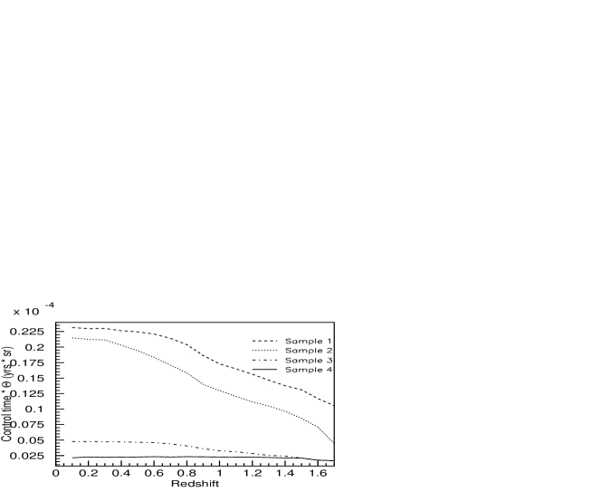
Figure 4: The product of the control time and surveyed area as a function of redshift for the four samples listed in Table 2, calculated for a stretch 1 Ia. The dashed line is for sample #1, where the 5 GOODS North epochs were used as the search data, and the combined 2004 ACS sample, as the reference. The dotted line is for sample #2, where the 4 epochs of the 2004 ACS dataset were used as the search data, and the combined GOODS North data, as the reference. The dashed-dotted line is for sample #3, where all 5 epochs of the GOODS South sample were used as the search data; and the combined epochs 4+5 of the South GOODS dataset, as the reference. The solid line is for sample #4, where all 5 epochs of the GOODS South sample were used as the search data; and the combined epochs 1+2 of the South GOODS dataset, as the reference.

There are several interesting features in Fig. 4. First, the product of the control time and area tends to decrease with redshift. This is a consequence of the fact that it becomes more difficult to satisfy the stage 2 SNR requirements for higher redshift (dimmer) supernovae. Second, for a given redshift, the product is smaller for sample #2 than for sample #1, a consequence of the fact that there are only 4 search epochs in sample #2 vs. 5 search epochs in sample #1. Third, the product is distinctly smaller for the South GOODS samples (samples #3 and #4) than for either of the North samples (#1 and #2), a reflection of the fact that for these samples we are forced to use references made from two of the GOODS South dataset’s own epochs. Finally, the product is smaller for sample #4, which uses epochs 1+2 of the GOODS South dataset as its reference data, than for it is for sample #5, which uses epochs 4+5. This is simply because the rise time of a supernova is smaller than its decline time.

4.2 Calculating $\epsilon_{\rm Ia}$ and $\epsilon_{\rm CC}$

In order to determine the efficiency of the stage 3 selection, we generate four Monte Carlo datasets simulating the data from the four datasets listed in Table 2 (in other words, they have the same sampling, exposure times, etc., as the data). Each Monte Carlo dataset contains 500 candidates for each of the 5 supernova types considered (Ia, Ibc, IIL, IIP, and IIn). The redshifts of these candidates are drawn from a Gaussian distribution that uses the redshifts and redshift errors of the real data events; the exposure times and sampling intervals also mimic those of the real data. The candidates’ rest-frame $B$-band magnitudes, stretch (for Type Ia’s), and extinction parameters are drawn from the appropriate distributions used in Eqns. 3.3 and 3.3. The time period between the date of explosion and the first observation is randomly drawn from a flat distribution. In addition, because we are simulating a dataset as it would appear by the time it is ready for the stage 3 selection, we impose the same selection requirements from stages 1 and 2 on these Monte Carlo events as we do on the real data.

After these Monte Carlo samples are generated, we calculate the number of candidates in each redshift bin. Dividing this number by the total number of the generated Ia’s yields the efficiency $\epsilon_{j\,{\rm Ia}}^{m}$, for redshift bin $j$ for Monte Carlo dataset $m$. Similarly, the efficiency for non-Type Ia candidates, $\epsilon_{j\,{\rm CC}}^{m}$, is defined as the sum of the probabilities of the non-Type Ia candidates divided by the total number of all generated non-Type Ia supernovae. The values of $\epsilon_{j\,{\rm Ia}}^{m}$’s range from $\sim$10 to 90%; and the values of $\epsilon_{j\,{\rm CC}}^{m}$’s, $\sim$3 to 50%, depending on the redshift bin.

4.3 Comparison of Expected and Observed Numbers of Supernovae

We can now put everything together and compute the expected numbers of supernovae for a given model of the Type Ia supernova rates using Eqn. 23. We calculate the observed numbers of supernovae for redshifts $\bar{z}$ $\leq$ 1.7, as well as the expected numbers of supernovae for the two models considered in Pain et al. (2002): a redshift-independent one and one evolving with redshift as a power law. We perform a least-squares fit of the observed numbers of supernovae to the predictions for both models. We also perform a maximum likelihood fit and compare the results.

• Redshift-independent rate. Assuming the rate is flat as a function of redshift, we obtain the best-fit value of ${\rm r_{V,Ia}}$ = (1.1 ${}^{+0.2}_{-0.2}$) $\times$ 10^-4 $N_{\rm Ia}$/(year Mpc³ $h_{70}^{-3}$) , with a $\chi^{2}$ = 11.5 for 16 degrees of freedom. Figure 5 (left) shows the resulting distribution of the predicted and observed numbers of supernovae. The errors on the predicted numbers of supernovae are a quadratic combination of the statistical and systematic errors (the statistical and systematic errors are comparable). The maximum likelihood method yields ${\rm r_{V,Ia}}$ = (0.7${}^{+0.2}_{-0.2}$) $\times$ 10^-4 $N_{\rm Ia}$/(year Mpc³ $h_{70}^{-3}$), consistent with the $\chi^{2}$ method.

• Rate evolving as a power law with redshift. Assuming the rate is varying as a function of redshift as (1 + $\bar{z}$)^α, using the $\chi^{2}$ fitter we obtain the best-fitting value for $\alpha$ = 0.2${}^{+0.7}_{-0.7}$ with a $\chi^{2}$ = 11.4 for 15 degrees of freedom. This is consistent with Pain et al. (2002), who found $\alpha$ = 0.8 $\pm$ 1.6. Note that the fit results are also consistent with the $\alpha$ = 0 case that was considered above. The maximum likelihood method yields $\alpha$ = -0.4${}^{1.0}_{1.1}$.

  Figure 5: Left: The total observed candidates for the 4 samples are plotted as a function of redshift (filled circles). The errors on the observed candidates are given in Table 8. The predicted number of candidates has been computed assuming a redshift-independent volumetric Type Ia rate of ${\rm r_{V,Ia}}(\bar{z})$ = 1.1 $\times$ 10^-4 $N_{\rm Ia}$/(year Mpc³ $h_{70}^{-3}$)]), and is plotted as a dashed histogram. The shaded region around the predicted numbers indicates the range of combined statistical and systematic errors. The contributions from the statistical and systematic errors are comparable. Right: The calculated rates as a function of redshift (filled circles), with overplotted fit results to the fits described in the text: redshift-independent rate (solid line) and power-law redshift dependent rate (dashed line). Note that the plot does not show the rates in the first redshift bin; this is because in this bin the rates are effectively unconstrained on the scale shown.

Both the redshift-independent model and the power-law model yield acceptable fit results, judging by the obtained $\chi^{2}$’s (note, however, that the data points in neighboring bins are correlated, leading to lower $\chi^{2}$ per DOF). The probability $p(\Delta\chi^{2}|\Delta DOF)$ = 0.1, where $\Delta\chi^{2}$ and $\Delta DOF$ are the difference in the $\chi^{2}$ and the numbers of degrees of freedom, respectively, for the redshift-independent model and the power-law model. In other words, the approximate probability that data would fluctuate from the redshift-independent model to the power-law model is 0.1. This fact indicates that our description of the experiment is good at both low and high redshifts. One must note, however, that at redshifts $>$ 1 the samples start becoming sparser, and at redshifts $>$  1.4 the measurement becomes particularly difficult with this dataset.

5 Comparison to Rates in the Literature

To compare our results with those of Dahlen et al. (2004), we now compute the Type Ia supernova rates in four large redshift bins, 0.2 $\leq$ $\bar{z}$ $<$ 0.6, 0.6 $\leq$ $\bar{z}$ $<$ 1.0, 1.0 $\leq$ $\bar{z}$ $<$ 1.4, and 1.4 $\leq$ $\bar{z}$ $<$ 1.7. Table 11 enumerates the estimates for the number of candidates in these redshift bins for the four samples listed in Table 2.

Redshift bin	$d_{j}^{1}$	$d_{j}^{2}$	$d_{j}^{3}$	$d_{j}^{4}$	Total
0.2 $\leq$ $z$ $<$ 0.6	2.40${}^{+3.07}_{-0.86}$ (0)	1.81${}^{+3.05}_{-0.60}$	0.00${}^{+1.17}_{-0.00}$ (0)	1.00${}^{+2.28}_{-0.28}$ (2)	5.44${}^{+3.90}_{-1.63}$
0.6 $\leq$ $z$ $<$ 1.0	13.40${}^{+8.28}_{-5.22}$ (6)	3.85${}^{+3.47}_{-1.25}$	1.71${}^{+2.90}_{-0.63}$ (2)	1.07${}^{+2.42}_{-0.30}$ (2)	18.33${}^{+4.62}_{-4.62}$
1.0 $\leq$ $z$ $<$ 1.4	3.23${}^{+3.07}_{-0.97}$ (3)	2.01${}^{+3.25}_{-0.75}$	1.50${}^{+2.74}_{-0.48}$ (1)	1.70${}^{+2.62}_{-0.58}$ (1)	8.87${}^{+3.13}_{-2.36}$
1.4 $\leq$ $z$ $<$ 1.7	0.00${}^{+1.13}_{-0.00}$ (0)	0.35${}^{+1.72}_{-0.35}$	0.00${}^{+1.13}_{-0.00}$ (1)	0.00${}^{+1.13}_{-0.00}$ (1)	0.35${}^{+1.72}_{-0.35}$

Table 11: The best estimate (i.e., the most probable) number of Ia’s, $d_{j}^{m}$, in $\Delta\bar{z}$ = 0.4 (0.3 for the last bin) redshift bins ($j$ = [1,..,4]), for the four samples listed in Table 2 ($m$ = [1,..,4]). The numbers in parenthesis are the number of gold and silver Ia’s in the sample from Riess et al. (2004a), that were used in the rates analysis of Dahlen et al. (2004). The total numbers are the results of applying the counting procedure described in the text to the combined candidates from all four samples (in other words, the total probability distribution is not a trivial sum of the probability distributions for the four samples). All the uncertainties reflect a 68% confidence region.

Using all four samples, we can now compute the rates for each bin using Eqn. 23. The values for $\Theta T(\bar{z})$, $dV/d\bar{z}$, $r_{V,\rm CC}/r_{V,\rm Ia}$, and $\bar{z}$ are taken in the middle of the bin. The errors on the rates are a quadratic combination of the errors on the number of observed Ia’s listed in Table 11, as well as statistical and systematic errors on the right-hand-side part of Eqn. 23. The resulting rates are summarized in Table 12 and plotted in Fig. 6 together with the rates from Dahlen et al. (2004) and results from the literature at lower redshifts. It is apparent that our results are consistent with those from the literature: in particular, at higher redshifts our rates are not inconsistent with those of Dahlen et al. (2004), although obtaining a precise measure of the consistency would require a careful evaluation of the correlations between the samples used in both analyses.

Redshift bin	${\rm r_{V,Ia}(\bar{z})}$
	([10-4 $N_{\rm Ia}$/(year Mpc3 $h_{70}^{-3}$)])
0.2 $\leq$ $\bar{z}$ $<$ 0.6	$0.53^{+0.39}_{-0.17}$
0.6 $\leq$ $\bar{z}$ $<$ 1.0	$0.93^{+0.25}_{-0.25}$
1.0 $\leq$ $\bar{z}$ $<$ 1.4	$0.75^{+0.35}_{-0.30}$
1.4 $\leq$ $\bar{z}$ $<$ 1.7	$0.12^{+0.58}_{-0.12}$

Table 12: The Type Ia supernova rates in the four redshift bins considered. The errors are a quadratic combination of the errors on $d_{j}^{m}$’s listed in Table 11, as well as statistical and systematic errors on the right-hand-side of Eqn. 23.

Figure 6: The filled circles are the results of this work. The first three empty squares at low redshifts (the “low-$z$ results”) are, from lower to higher redshifts, the results of Cappellaro et al. (1999), Madgwick et al. (2003), and Blanc et al. (2004), respectively. The open upturned triangle at $z$ = 0.47 is from Neill et al. (2006). The open circle at $z$ = 0.50 is from Tonry et al. (2003). The open star at $z$ = 0.55 is from Pain et al. (2002). The open diamonds are the results of Barris and Tonry (2006). The crosses are from Dahlen et al. (2004) (including systematic errors). The horizontal bars are estimated redshift bin sizes.

Note that Type Ia supernovae that we have considered encompass a wide range of magnitudes, stretch parameters, extinction possibilities, etc.. Therefore, the procedure described in section 3.3 accounts for not only the more standard Type Ia’s (such as those described in Branch et al. (1993)), but also non-standard Type Ia’s, such as type 1991bg and 1991T Filippenko et al. (1992). 1991bg-like supernovae have low values of the stretch parameter ($s$ = 0.71 $\pm$ 0.05), and are typically $\sim$1.7 magnitudes fainter in the $V$-band and $\sim$2.6 magnitudes fainter in the $B$-band. Stretch values of 0.71 are certainly within the range of the stretch parameters we considered; as for the magnitudes, it is reassuring to note that the case of strong extinction ($A_{V}$ = 1) did not significantly alter our results (see Table 9). 1991T-like supernovae are about 0.5-0.9 magnitudes brighter than normal Ia’s, with stretch $s$ = 1.07 $\pm$ 0.06. Both the stretch and the magnitude values are well within the considered ranges of these parameters. Note also that the fact that the Bayesian classification method was able to accurately type the vast majority of the 73 Type Ia candidates from the SNLS dataset, as was demonstrated in Kuznetsova and Connolly (2007), shows that the method is capable of identifying Type Ia’s in large populations that presumably include non-standard Ia’s.

It is particularly interesting to compare our rate results with that of Dahlen et al. (2004). That study also analyzed the GOODS sample, but there are important differences in our methods, as pointed out above (Sec. 1). While our results are in statistical agreement, our measured rate in a given bin can differ from theirs through either the candidate counting or the calculation of the control time/efficiency.

• Candidate counting: In some bins, the final count of the candidates ends up being about the same for both analyses, but the actual candidates are not the same. This is not unexpected because the techniques used for the supernova identification in the two analyses are quite different. Our method provides a probabilistic rather than an absolute identification of each individual supernova based on its photometric measurements alone; the same probabilistic approach is used for calculating the efficiency and mis-identification.

  For example, in the highest redshift bin, we have one candidate but this is from Sample 2, which was taken after the work of Dahlen et al. (2004) was published. However, the two high-redshift Ia candidates from Samples 3 and 4, SN-2002fx and SN-2003ak, which were used in Dahlen et al. (2004), did not pass our stage 2 cuts.

• Control time/efficiency: A rigorous comparison of the control times is difficult due to the lack of tabulated control time data in Dahlen et al. (2004). However, a rough estimation of the control time times efficiency factor from the data given in Dahlen et al. (2004) shows that this factor is approximately half our values for all but the highest redshift bin.

6 The Star Formation History Connection

A particularly interesting aspect of a Type Ia supernova rates analysis is the possibility of constraining the delay time between the formation of a progenitor star and a supernova explosion, which in turn helps constrain possible models for the Type Ia supernova formation. There are two leading models that have been considered in the recent literature: the so-called two-component model and a Gaussian delay model. We will now consider both of these models. Unlike section 4.3, now that we are considering the rates we can add the low-redshift measurements of Cappellaro et al. (1999), Madgwick et al. (2003), and Blanc et al. (2004) to our results and use the combined data in the fits.

The two-component model (Scannapieco and Bildstren, 2005; Mannucci et al., 2006) suggests that that the delay function may be bimodal, with one component responsible for the “prompt” Type Ia supernovae that explode soon after the formation of their progenitors; and the other, for the “tardy” supernovae that have a much longer delay time. Following this model, the Type Ia supernova rate can be represented as:

$${\rm r_{V,Ia}(\bar{z})}=A\rho_{\ast}(\bar{z})+B\dot{\rho}_{\ast}(\bar{z}),$$ (28)

where $\rho_{\ast}(\bar{z})$ is the integrated SFH and $\dot{\rho}_{\ast}(\bar{z})$ is the instantaneous SFH. The first term of the equation accounts for the “tardy” population, while the second, for the “prompt” one. We use the parametric form of the SFH as given in Hopkins and Beacom (2006):

$$\dot{\rho}_{\ast}(\bar{z})=\frac{(a+b\bar{z})\,h_{70}}{1+(\bar{z}/c)^{d}},$$ (29)

where $h_{70}=0.7$, $a$ = 0.017, $b$ = 0.13, $c$ = 3.3, $d$ = 5.3.

The Levenberg-Marquardt least-squares fit of the combined data to the two-component model is shown in Fig. 7 (left). We obtain $A$ = (1.5 $\pm$ 0.7) $\times 10^{-14}$ yr^-1M${}_{\odot}^{-1}$ and $B$ = (5.4 $\pm$ 2.0) $\times 10^{-4}$ yr^-1/(M_⊙ yr^-1). These results are entirely consistent with those obtained by Neill et al. (2006): $A$ = (1.4 $\pm$ 1.0) $\times 10^{-14}$ yr^-1M${}_{\odot}^{-1}$ and $B$ = (8.0 $\pm$ 2.6) $\times 10^{-4}$ yr^-1/(M_⊙ yr^-1). The $\chi^{2}$ of the fit is 5.4 for 5 degrees of freedom.

Note that the results of Barris and Tonry (2006) at $z$ = 0.55, 0.65, and 0.75 are somewhat inconsistent with our best-fitting two-component model, with the discrepancy at the level of 4.1, 3.2, and 5.2 $\sigma$, respectively. This can be seen from Fig. 6. It has been argued in Neill et al. (2006) (who also noted that the results of Barris and Tonry (2006) beyond the redshift of 0.5 appear to be rather high) that contamination by non-Type Ia’s is the most likely source of the problem.

It was suggested in Dahlen et al. (2004) and Strolger et al. (2004) that the Ia rate is a convolution of the SFH and a Gaussian time delay distribution function with a characteristic time delay $\tau$ $\sim$3 Gyr and a $\sigma$ = 0.2 $\tau$. Using the Hopkins-Beacom SFH, we find that the best-fitting parameters for such a model are $\tau$ = (3.2 $\pm$ 0.6) Gyr and $\sigma$ = (0.12 $\pm$ 0.54) $\tau$, with a fit $\chi^{2}$ of 2.1 for 4 degrees of freedom. The fit is shown in Fig. 7 (right). For comparison, we also show the rate model obtained using the parameters from Strolger et al. (2004) ($\tau$ = 3 Gyr and $\sigma$ = 0.2 $\tau$).

Figure 7: Left: The least-square fit of the two-component model to the data. The dashed line represents the prompt component that is proportional to the instantaneous SFH. The dotted line represents the tardy component that is proportional to the integrated SFH. The thick solid line is the sum of the two. Right: The Gaussian time delay model with our best-fitted parameters (solid line), as well as with the parameters of Strolger et al. (2004) (dashed line). In both plots, the first three empty squares at low redshifts are, from lower to higher redshifts, the results of Cappellaro et al. (1999), Madgwick et al. (2003), and Blanc et al. (2004), respectively. The filled circles are the results of this work. The horizontal bars are estimated redshift bin sizes.

One of the main differences between the two-component model and the time delay model is the predicted behavior at high redshifts: the former predicts an increase in the rates, while the latter, a decrease. From Fig. 7 and the results of the fits of our data to both models, we find that neither scenario can be ruled out.

7 Summary

We have analyzed the rates of Type Ia supernovae up to a redshift of 1.7 using two samples collected with the HST: the GOODS data, and the 2004 ACS sample collected in the Spring-Summer 2004 covering the GOODS North field. Using only the data from two broadband filters, F775W and F850LP, we applied a novel technique for identifying Type Ia supernovae based on a Bayesian probability approach. This method allows us to automatically type supernova candidates in large samples, properly taking into account all known sources of systematic error. We also make use of the best currently available full spectral templates for five different supernova types for the candidate typing, as well as for calculating the efficiency of our supernova search, and the control time. These templates will undoubtedly be improved over the next several years as more supernova data becomes available. Current and upcoming supernova surveys will not only provide a better understanding of individual supernova types, but may also uncover new types of supernovae, which can then be added to the Bayesian classification framework. Likewise, a better understanding of the many parameters that affect supernova observations will improve the classification scheme, which will result in better constraints on the measured rates. The calculations of the supernova finding efficiency, the control time, and the survey area are all done taking into account the specific observing configurations pertinent for the surveys, such as exposure times, cadences, and the orientations of the GOODS tiles.

We carried out a comparison of the predicted and observed numbers of supernovae in redshift bins of $\Delta\bar{z}$ = 0.1, for two different models of the Type Ia supernova rates: a redshift-independent rate and a power-law redshift-dependent rate. We find that the available data fit both models equally well.

For comparison with previous work, particularly that of Dahlen et al. (2004), who also analyzed a large subset of the data used here, we calculated the volumetric Type Ia supernova rates in four redshift bins, 0.2 $\leq$ $\bar{z}$ $<$ 0.6, 0.6 $\leq$ $\bar{z}$ $<$ 1.0, 1.0 $\leq$ $\bar{z}$ $<$ 1.4, and 1.4 $\leq$ $\bar{z}$ $<$ 1.7. We find that our results are generally consistent with those of Dahlen et al. (2004). Due to the larger of number supernova candidates which this Bayesian classification technique makes available, we obtain smaller or equal uncertainties in all the bins up to $z$ = 1.7. In the highest redshift bin we obtain a larger uncertainty because the signal to noise ratio is generally too low to apply this technique.

We fitted the resulting rates to two leading models used in recent literature: the two-component model and a Gaussian time delay model. The former model implies an increase in the Type Ia supernova rates at highest redshifts; while the latter, a decrease. We find that the statistics of the present sample does not definitively discriminate between the two scenarios – only one supernova in this work and two supernovae in Dahlen et al. (2004) contribute to the important highest-redshift bin. Significantly larger surveillance time would be required to arrive at a conclusive statement on the trends for the Type Ia rates at high redshifts.

In the future, several ambitious new surveys are planned that will collect photometric data for thousands of supernovae in order to improve the constraints on dark energy. Individual spectroscopic follow up for every supernova candidate is likely to be impractical in these surveys. The Bayesian classification method described here has the ability to classify supernovae using photometric measurements alone, and is a promising technique for these future surveys.

8 Acknowledgments

We would like to thank Tomas Dahlen and Bahram Mobasher for providing us with photometric redshifts for a number of supernova candidates. We would also like to thank the anonymous referee for the many insightful comments and suggestions. Financial support for this work was provided by NASA through program GO-9727 from the Space Telescope Science Institute, which is operated by AURA, Inc., under NASA contract NAS 5-26555. This work was also partially supported by the Director, Office of Science, Department of Energy, under grant DE-AC02-05CH11231.

References

- Aldering et al. (2004) Aldering, G., et al. 2004, submitted to PASP, preprint astro-ph/0405232
- Alexander et al. (2003) Alexander, D. M., et al. 2003, AJ, 126, 1772
- Astier et al. (2006) Astier, P, et al. 2006, A&A, 447, 31
- Barris and Tonry (2006) Barris, B. J., & Tonry, J. L., 2006, ApJ, 637, 427
- Bertin and Arnouts (1996) Berin, E., & Arnouts, S., 1996, A&A, 117, 393
- Blanc et al. (2004) Blanc, G., et al. 2004, A&A, 423, 881
- Branch et al. (1993) Branch, D., Fisher, A., Nugent, P. E., 1993, AJ, 106, 2383
- Cardelli et al. (1998) Cardelli, J. A., Clayton, G. C., & Mathis, J. S., 1988, ApJ, 329, L33
- Cappellaro et al. (1999) Cappellaro, E., Evans, R., & Turatto, M., 1999, A&A, 351, 459
- Chandrasekhar (1931) Chandrasekhar, S., 1931, ApJ, 74, 81
- Cohen et al. (2000) Cohen, J. G., et al. 2000, ApJ, 538, 29
- Cowie et al. (2004) Cowie, L. L., et al. 2004, AJ, 127, 3137
- Dahlen et al. (2004) Dahlen, T., et al. 2004, ApJ, 613, 189
- Dahlen and Fransson (1999) Dahlen, T., & Fransson, C., 1999, A&A 350, 349
- Dickinson et al. (2003) Dickinson, M., et al. 2003, in The Mass of Galaxies at Low and High Redshift, ed. R. Bender and A. Renzini (Berlin: Springer), 324
- Filippenko et al. (1992) Filippenko, A. V., et al. 1992, AJ, 104, 1543F
- Fruchter and Hook (2002) Fruchter, A., & Hook, R. N., 2002, PASP, 114, 144
- Giavalisco et al. (2004) Giavalisco, M., et al. 2004, ApJ 600, L93
- Hardin et al. (2000) Hardin, D., et al. 2000, A&A, 362, 419
- Hatano et al. (1998) Hatano, K., Branch, D., & Deaton, J., 1998, ApJ, 502, 177
- Hopkins and Beacom (2006) Hopkins, A. M., & Beacom, J. F., 2006, ApJ, 651, 142
- Hornschemeier et al. (2003) Hornschemeier, A. E., et al. 2003, AJ, 126, 575
- Johnson and Crotts (2006) Johnson, B. D., and Crotts, A. P. S., 2006, ApJ, 132, 756
- Kashikawa et al. (2002) Kashikawa, N., et al. 2002, PASJ, 54, 819
- Krist and Hook (2004) Krist, J., & Hook, R., 2004, The TinyTim User’s Guide, STScI, 339
- Kuznetsova and Connolly (2007) Kuznetsova, N. & Connolly, B. M., 2007, ApJ, 659, 530
- Le Fevre et al. (2004) Le Fèvre, O., et al. 2004, A&A, 428, 1043
- Madgwick et al. (2003) Madgwick, D. S., et al., 2003, ApJ 599, L33
- Mannucci et al. (2006) Mannucci, F., Della Valle, M., & Panagia, N., 2006, MNRAS, 370, 773
- Mobasher and Dahlen (2004) Mobasher, B., & Dahlen, T., private communications
- Neill et al. (2006) Neill, J. D, et al. 2006, AJ, 132, 1126
- Pain et al. (2002) Pain, R., et al. 2002, ApJ, 577, 120
- Pain et al. (1996) Pain, R. et al. 1996, ApJ, 473, 356
- Perlmutter et al. (1997) Perlmutter, S., et al. 1997, ApJ, 483, 565
- Perlmutter et al. (1999) Perlmutter, S., et al. 1999, ApJ, 517, 565
- for review, see Perlmutter and Schmidt (2003) Perlmutter, S., & Schmidt, B. P., 2003, in Supernovae and Gamma Ray Bursts, ed K. Weiler (Berlin: Springer), 598
- Poznanski et al. (2002) Poznanski, D. et al., 2002, PASP, 114, 833
- Renzini et al. (2002) Renzini, A., et al. 2003, in The Mass of Galaxies at Low and High Redshift, ed. R. Bender and A. Renzini (Berlin: Springer), 332
- Richardson et al. (2002) Richardson, D.,et al. 2002, AJ, 123, 745
- Richardson et al. (2006) Richardson, D. et al. 2006, AJ, 131, 2233
- for more recent treatment, see also Riello and Patat (2005) Riello, M, & Patat, F., 2005, Mon. Not. Roy. Astron. Soc., 362, 671
- Riess et al. (1998) Riess, A. G., et al. 1998, AJ, 116, 1009
- Riess et al. (2004a) Riess, A. G., et al. 2004a, ApJ, 607, 665
- Riess et al. (2004b) Riess, A. G., et al., 2004b, ApJ, 600, L163
- Riess et al. (2007) Riess. A. G., et al. 2007, ApJ, 659, 98
- Rosati et al. (2002) Rosati, P., et al., 2002, ApJ. Suppl. 139, 369
- Scannapieco and Bildstren (2005) Scannapieco, E., and Bildstren, L., 2005, ApJ, 629, L85
- Strolger et al. (2004) Strolger, L.-G., et al. 2004, ApJ, 613, 200
- Sullivan et al. (2005) Sullivan, M., et al., 2006, AJ, 131, 960
- Sullivan et al. (2006) Sullivan, M., et al. 2006, ApJ, 648, 868
- Suzuki et al. (2008) Suzuki, N., et al. 2008, in preparation
- Tonry et al. (2003) Tonry, J. L., et al. 2003, ApJ, 594, 1
- van Dokkum (2001) van Dokkum, P. G., 2001, PASP, 113, 1420
- Vanzella et al. (2006) Vanzella, E., et al. 2006, A&A, 454, 423
- Wirth (2004) Wirth, G. D., et al. 2004, AJ, 127, 3121
- Wolf et al. (2004) Wolf, C., et al. 2004, A&A, 421, 913