Heavy MSSM Higgs Bosons at CMS:
“LHC wedge” and Higgs-Mass Precision

Abstract

The search for MSSM Higgs bosons will be an important goal at the LHC. In order to analyze the search reach of the CMS experiment for the heavy neutral MSSM Higgs bosons, we combine the latest results for the CMS experimental sensitivities based on full simulation studies with state-of-the-art theoretical predictions of MSSM Higgs-boson properties. The experimental analyses are done assuming an integrated luminosity of 30 or 60 $\mbox{fb}^{-1}$. The results are interpreted as 5$\,\sigma$ discovery contours in MSSM $M_{A}$–$\tan\beta$ benchmark scenarios. Special emphasis is put on the variation of the Higgs mixing parameter $\mu$. While the variation of $\mu$ can shift the prospective discovery reach (and correspondingly the “LHC wedge” region) by about $\Delta\tan\beta=10$, the discovery reach is rather stable with respect to the impact of other supersymmetric parameters. Within the discovery region we analyze the accuracy with which the masses of the heavy neutral Higgs bosons can be determined. An accuracy of 1–4% should be achievable, depending on $M_{A}$ and $\tan\beta$.

1 Introduction

Identifying the mechanism of electroweak symmetry breaking will be one of the main goals of the LHC. The most popular models are the Higgs mechanism within the Standard Model (SM) and within the Minimal Supersymmetric Standard Model (MSSM) mssm . Contrary to the case of the SM, in the MSSM two Higgs doublets are required. This results in five physical Higgs bosons instead of the single Higgs boson of the SM. These are the light and heavy ${\cal CP}$-even Higgs bosons, $h$ and $H$, the ${\cal CP}$-odd Higgs boson, $A$, and the charged Higgs boson, $H^{\pm}$. The Higgs sector of the MSSM can be specified at lowest order in terms of the gauge couplings, the ratio of the two Higgs vacuum expectation values, $\tan\beta\equiv v_{2}/v_{1}$, and the mass of the ${\cal CP}$-odd Higgs boson, $M_{A}$. Consequently, the masses of the ${\cal CP}$-even neutral Higgs bosons and the charged Higgs boson are dependent quantities that can be predicted in terms of the Higgs-sector parameters. Higgs-phenomenology in the MSSM is strongly affected by higher-order corrections, in particular from the sector of the third generation quarks and squarks, so that the dependencies on various other MSSM parameters can be important.

The current exclusion bounds within the MSSM LEPHiggsMSSM ; D0bounds ; CDFbounds and the prospective sensitivities at the LHC are usually displayed in terms of the parameters $M_{A}$ and $\tan\beta$ that characterize the MSSM Higgs sector at lowest order. The other MSSM parameters are conventionally fixed according to certain benchmark scenarios benchmark2 ; benchmark3 . We focus here cmsHiggs on the $5\,\sigma$ discovery contours for heavy MSSM Higgs bosons, i.e. the lower bound of the “LHC wedge”, within the “$m_{h}^{\rm max}$ scenario”. For the interpretation of the exclusion bounds and prospective discovery contours in the benchmark scenarios it is important to assess how sensitively the results depend on those parameters that have been fixed according to the benchmark prescriptions. Consequently, we investigate how the 5$\,\sigma$ discovery regions in the $M_{A}$–$\tan\beta$ plane for the heavy neutral MSSM Higgs bosons obtainable with the CMS experiment at the LHC depend on the other MSSM parameters.

2 The analysis

The search for the heavy neutral MSSM Higgs bosons at the LHC will mainly be pursued in the $b$ quark associated production with a subsequent decay to $\tau$ leptons lhctdrsA ; atlashiggs ; lhctdrsS . In the region of large $\tan\beta$ this production process benefits from an enhancement factor of $\tan^{2}\beta\hskip 2.84526pt$ compared to the SM case. The main search channels are (here and in the following $\phi$ denotes the two heavy neutral MSSM Higgs bosons, $\phi=H,A$):

$$b\bar{b}\phi,\phi\to\tau^{+}\tau^{-}\to 2\,\mbox{jets}$$ (1)

$$b\bar{b}\phi,\phi\to\tau^{+}\tau^{-}\to\mu+\,\mbox{jet}$$ (2)

$$b\bar{b}\phi,\phi\to\tau^{+}\tau^{-}\to e+\,\mbox{jet}$$ (3)

The analyses were performed with full CMS detector simulation and reconstruction for the following three final states of di-$\tau$-lepton decays: $\tau^{+}\tau^{-}\to\,\mbox{jets}$ CMSPTDRjj , $\tau^{+}\tau^{-}\to e+\,\mbox{jet}$ CMSPTDRej and $\tau^{+}\tau^{-}\to\mu+\mbox{jet}$ CMSPTDRmj . The Higgs-boson production in association with $b$ quarks, $pp\to b\bar{b}\phi$, has been selected using single $b$-jet tagging in the experimental analysis. The kinematics of the $gg\to b\bar{b}\phi$ production process (2 $\to$ 3) was generated with PYTHIA PYTHIA . The backgrounds considered in the analysis were QCD muli-jet events (for the $\tau\tau\to\,\mbox{jets}$ mode), $t\bar{t},b\bar{b}$, Drell-Yan production of $Z,\gamma^{\ast}$, $W$+jet, $Wt$ and $\tau\tau b\bar{b}$. All background processes were generated using PYTHIA, except for $\tau^{+}\tau^{-}b\bar{b}$, which was generated using CompHEP Boos:2004kh .

$\phi\to\tau^{+}\tau^{-}\to\,\mbox{jets}$, 60 $\mbox{fb}^{-1}$
$M_{A}$ [GeV]	200	500	800
$N_{S}$	63	35	17
$\varepsilon_{\rm exp}$	$2.5\times 10^{-4}$	$2.4\times 10^{-3}$	$3.6\times 10^{-3}$
$R_{M_{\phi}}$	0.176	0.171	0.187
$\Delta M_{\phi}/M_{\phi}$ [%]	2.2	2.8	4.5

Table 1: Required number of signal events, $N_{S}$, with ${\cal L}=60$ $\mbox{fb}^{-1}$ for a 5$\,\sigma$ discovery in the channel $\phi\to\tau^{+}\tau^{-}\to\,\mbox{jets}$. Furthermore given are the total experimental selection efficiency, $\varepsilon_{\rm exp}$, the ratio of the di-$\tau$ mass resolution to the Higgs-boson mass, $R_{M_{\phi}}$, and the expected precision of the Higgs-boson mass measurement, $\Delta M_{\phi}/M_{\phi}$, obtainable from $N_{S}$ signal events.

$\phi\to\tau^{+}\tau^{-}\to e+\,\mbox{jet}$, 30 $\mbox{fb}^{-1}$
$M_{A}$ [GeV]	200	300	500
$N_{S}$	72.9	45.5	32.8
$\varepsilon_{\rm exp}$	$3.0\times 10^{-3}$	$6.4\times 10^{-3}$	$1.0\times 10^{-2}$
$R_{M_{\phi}}$	0.216	0.214	0.230
$\Delta M_{\phi}/M_{\phi}$ [%]	2.5	3.2	4.0

Table 2: Required number of signal events, $N_{S}$, with ${\cal L}=30$ $\mbox{fb}^{-1}$ for a 5$\,\sigma$ discovery in the channel $\phi\to\tau^{+}\tau^{-}\to e+\,\mbox{jet}$. The other quantities are defined as in Tab. 1.

$\phi\to\tau^{+}\tau^{-}\to\mu+\,\mbox{jet}$, 30 $\mbox{fb}^{-1}$
$M_{A}$ [GeV]	200	500
$N_{S}$	79	57
$\varepsilon_{\rm exp}$	$7.0\times 10^{-3}$	$2.0\times 10^{-2}$
$R_{M_{\phi}}$	0.210	0.200
$\Delta M_{\phi}/M_{\phi}$ [%]	2.4	2.6

Table 3: Required number of signal events, $N_{S}$, with ${\cal L}=30$ $\mbox{fb}^{-1}$ for a 5$\,\sigma$ discovery in the channel $\phi\to\tau^{+}\tau^{-}\to\mu+\,\mbox{jet}$. The other quantities are defined as in Tab. 1.

The results quoted in Tabs. 1 – 3 for the required number of signal events depend only on the Higgs-boson mass, i.e. the event kinematics, but are independent of any specific MSSM scenario. In order to determine the 5$\,\sigma$ discovery contours in the $M_{A}$–$\tan\beta$ plane these results have to be confronted with the MSSM predictions. The number of signal events, $N_{\rm ev}$, for a given parameter point is evaluated via

$$N_{\rm ev}={\cal L}\times\sigma_{b\bar{b}\phi}\times{\rm BR}(\phi\to\tau^{+}\tau^{-})\times{\rm BR}_{\tau\tau}\times\varepsilon_{\rm exp}~{}.$$ (4)

Here ${\cal L}$ denotes the luminosity collected with the CMS detector, $\sigma_{b\bar{b}\phi}$ is the Higgs-boson production cross section, ${\rm BR}(\phi\to\tau^{+}\tau^{-})$ is the branching ratio of the Higgs boson to $\tau$ leptons, ${\rm BR}_{\tau\tau}$ is the product of the branching ratios of the two $\tau$ leptons into their respective final state,

$${\rm BR}(\tau\to\,\mbox{jet}+X) \approx 0.65~{},$$ (5)

$${\rm BR}(\tau\to\mu+X)\approx{\rm BR}(\tau\to e+X) \approx 0.175~{},$$ (6)

and $\varepsilon_{\rm exp}$ denotes the total experimental selection efficiency for the respective process (as given in Tabs. 1 – 3). For our numerical predictions of total cross sections (see Ref. sigmaFH and references therein) and branching rations of the MSSM Higgs bosons we use the program FeynHiggs feynhiggs ; mhiggslong ; mhiggsAEC ; mhcMSSMlong . We take into account effects from higher-order corrections and from decays of the heavy Higgs bosons into supersymmetric particles.

In spite of the escaping neutrinos, the Higgs-boson mass can be reconstructed in the $H,A\to\tau\tau$ channel from the visible $\tau$ momenta ($\tau$ jets) and the missing transverse energy, $E_{\rm T}^{\rm miss}$, using the collinearity approximation for neutrinos from highly boosted $\tau$’s. In the investigated region of $M_{A}$ and $\tan\beta$ the two states $A$ and $H$ are nearly mass-degenerate. For most values of the other MSSM parameters the mass difference of $A$ and $H$ is much smaller than the achievable mass resolution, and the difference in reconstructing the $A$ or the $H$ will have no relevant effect on the achievable accuracy in the mass determination. The precision $\Delta M_{\phi}/M_{\phi}$ shown in Tabs. 1 – 3 is derived for the border of the parameter space in which a 5$\,\sigma$ discovery can be claimed, i.e. with $N_{S}$ observed Higgs events. The statistical accuracy of the mass measurement has been evaluated via

$${\Delta M_{\phi}}/{M_{\phi}}={R_{M_{\phi}}}/{\sqrt{N_{S}}}~{}.$$ (7)

A higher precision can be achieved if more than $N_{S}$ events are observed. The corresponding estimate for the precision is obtained by replacing $N_{S}$ in eq. (7) by the number of observed signal events, $N_{\rm ev}$. It should be noted that the prospective accuracy obtained from eq. (7) does not take into account the uncertainties of the jet and missing $E_{\rm T}$ energy scales. In the $\tau^{+}\tau^{-}\to\,\mbox{jets}$ mode these effects can lead to an additional 3% uncertainty in the mass measurement CMSPTDRjj .

3 Numerical results for the LHC wedge

We have evaluated $N_{\rm ev}$ in the $m_{h}^{\rm max}$ benchmark scenario benchmark2 ; benchmark3 as a function of $M_{A}$ and $\tan\beta$. For fixed $M_{A}$ we have varied $\tan\beta$ such that $N_{\rm ev}=N_{S}$ (as given in Tabs. 1 – 3). This $\tan\beta$ value is then identified as the point on the 5$\,\sigma$ discovery contour corresponding to the chosen value of $M_{A}$. In this way we have determined the 5$\,\sigma$ discovery contours for the $m_{h}^{\rm max}$ scenario for $\mu=\pm 200,\pm 1000\,\,\mathrm{GeV}$.

In Fig. 1 we show the $5\sigma$ discovery contours obtained from the process $b\bar{b}\phi,\phi\to\tau^{+}\tau^{-}$ for the final states $\tau^{+}\tau^{-}\to\,\mbox{jets}$, $\tau^{+}\tau^{-}\to e+\,\mbox{jet}$ and $\tau^{+}\tau^{-}\to\mu+\,\mbox{jet}$. The 5$\,\sigma$ discovery contours are affected by a change in $\mu$ in two ways. Higher-order contributions, in particular the ones associated with $\Delta_{b}$ deltamb2 , modify the Higgs-boson production cross sections and decay branching ratios. Furthermore the mass eigenvalues of the charginos and neutralinos vary with $\mu$, possibly opening up the decay channels of the Higgs bosons to supersymmetric particles, which reduces the branching ratio to $\tau$ leptons.

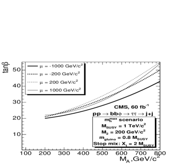
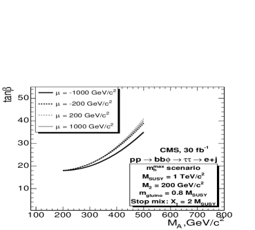
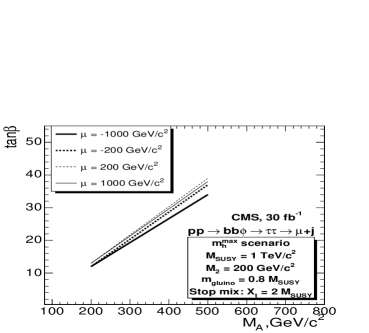
Figure 1: Variation of the $5\sigma$ discovery contours obtained in the $m_{h}^{\rm max}$ scenario for different values of $\mu$ from the channels $b\bar{b}\phi,\phi\to\tau^{+}\tau^{-}\to\,\mbox{jets}$ (top), $\to e+\,\mbox{jet}$ (middle), $\to\mu+\,\mbox{jet}$ (bottom).

As expected from the discussion of the $\Delta_{b}$ corrections in Refs. benchmark3 ; cmsHiggs , the variation of the 5$\,\sigma$ discovery contours with $\mu$ can be sizable. In the $\tau^{+}\tau^{-}\to\,\mbox{jets}$ channle (top plot in Fig. 1) a shift up to $\Delta\tan\beta=12$ can be observed for $M_{A}=800\,\,\mathrm{GeV}$. For low $M_{A}$ values (corresponding also to lower $\tan\beta$ values on the discovery contours) the variation stays below $\Delta\tan\beta=3$. In the no-mixing scenario the variation does not exceed $\Delta\tan\beta=5$. The 5$\,\sigma$ discovery regions are largest for $\mu=-1000\,\,\mathrm{GeV}$ and pushed to highest $\tan\beta$ values for $\mu=+200\,\,\mathrm{GeV}$. In the low $M_{A}$ region our discovery contours are very similar to those obtained in Ref. benchmark3 . In the high $M_{A}$ region, $M_{A}\sim 800\,\,\mathrm{GeV}$, corresponding to larger values of $\tan\beta$ on the discovery contours, our improved evaluation of the 5$\,\sigma$ discovery contours gives rise to a shift towards higher $\tan\beta$ values compared to Ref. benchmark3 of about $\Delta\tan\beta=8$ (mostly due to the up-to-date experimental input).

The results for the channel $\tau^{+}\tau^{-}\to e+\,\mbox{jet}$ are shown in the middle plot of Fig. 1. The resulting shift in $\tan\beta$ reaches up to $\Delta\tan\beta=8$ for $M_{A}=500\,\,\mathrm{GeV}$. Finally in the bottom plot of Fig. 1 the results for the channel $\tau^{+}\tau^{-}\to\mu+\,\mbox{jet}$ are depicted. The level of variation of the 5$\,\sigma$ discovery contours is the same as for the $e+\,\mbox{jet}$ final state.

In Ref. cmsHiggs it has been shown that the effects visible in Fig. 1 arising from the variation of $\mu$ are a mixture of two effects: the change in the bottom Yukawa coupling via $\Delta_{b}$ and the impact on the heavy Higgs decay channels of possible additional decays to charginos or neutralinos. The variation of other parameters entering the radiative corrections is comparably small.

4 Numerical results for the Higgs-boson mass precision

The expected statistical precision of the heavy Higgs-boson masses is evaluated according to eq. (7). In Fig. 2 we show the expected precision for the mass measurement achievable from the channel $b\bar{b}\phi,\phi\to\tau^{+}\tau^{-}$ using the final state $\tau^{+}\tau^{-}\to\,\mbox{jets}$. Within the 5$\,\sigma$ discovery region we have indicated contour lines corresponding to different values of the expected precision, $\Delta M/M$. The results are shown in the $m_{h}^{\rm max}$ benchmark scenario for $\mu=-200\,\,\mathrm{GeV}$ (upper plot) and $\mu=+200\,\,\mathrm{GeV}$ (lower plot). We find that experimental precisions of $\Delta M_{\phi}/M_{\phi}$ of 1–4% are reachable within the discovery region. A better precision is reached for larger $\tan\beta$ and smaller $M_{A}$ as a consequence of the higher number of signal events in this region. The other channels and other values of $\mu$ discussed above yield qualitatively similar results to those shown in Fig. 2.

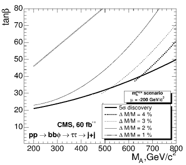
Figure 2: The statistical precision of the Higgs-boson mass measurement achievable from the channel $b\bar{b}\phi,\phi\to\tau^{+}\tau^{-}\to\,\mbox{jets}$ in the $m_{h}^{\rm max}$ benchmark scenario for $\mu=-200\,\,\mathrm{GeV}$ (top) and $\mu=+200\,\,\mathrm{GeV}$ (bottom) is shown together with the 5$\,\sigma$ discovery contour.

Acknowledgements

We thank S. Gennai, A. Kalinowski, R. Kinnunen and S. Lehti for collaboration on the work presented here. Work supported in part by the European Community’s Marie-Curie Research Training Network under contract MRTN-CT-2006-035505 ‘Tools and Precision Calculations for Physics Discoveries at Colliders’.

References

- (1) H. Nilles, Phys. Rept. 110 (1984) 1; H. Haber and G. Kane, Phys. Rept. 117 (1985) 75; R. Barbieri, Riv. Nuovo Cim. 11 (1988) 1.
- (2) [LEP Higgs working group], Eur. Phys. J. C 47 (2006) 547 [arXiv:hep-ex/0602042].
- (3) V. Abazov et al. [D0 Collaboration], Phys. Rev. Lett. 95 (2005) 151801 [arXiv:hep-ex/0504018]; Phys. Rev. Lett. 97 (2006) 121802 [arXiv:hep-ex/0605009]; D0 Note 5331-CONF.
- (4) A. Abulencia et al. [CDF Collaboration], Phys. Rev. Lett. 96 (2006) 011802 [arXiv:hep-ex/0508051]; CDF note 8676.
- (5) M. Carena, S. Heinemeyer, C. Wagner and G. Weiglein, Eur. Phys. J. C 26 (2003) 601 [arXiv:hep-ph/0202167].
- (6) M. Carena, S. Heinemeyer, C. Wagner and G. Weiglein, Eur. Phys. J. C 45 (2006) 797 [arXiv:hep-ph/0511023].
- (7) S. Gennai, S. Heinemeyer, A. Kalinowski, R. Kinnunen, S. Lehti, A. Nikitenko and G. Weiglein, to appear in Eur. Phys. J. C, arXiv:0704.0619 [hep-ph].
- (8) ATLAS Collaboration, Detector and Physics Performance Technical Design Report, CERN/LHCC/99-15 (1999).
- (9) K. Cranmer, Y. Fang, B. Mellado, S. Paganis, W. Quayle and S. Wu, hep-ph/0401148.
-
(10)
CMS Physics Technical Design Report, Volume 2. CERN/LHCC 2006-021,
see:
cmsdoc.cern.ch/cms/cpt/tdr/ . - (11) M. Albrow and A. Rostovtsev, [arXiv:hep-ph/0009336]; V. Khoze, A. Martin and M. Ryskin, Eur. Phys. J. C 23 (2002) 311 [arXiv:hep-ph/0111078]; A. De Roeck, V. Khoze, A. Martin, R. Orava and M. Ryskin, Eur. Phys. J. C 25 (2002) 391 [arXiv:hep-ph/0207042]; B. Cox, AIP Conf. Proc. 753 (2005) 103, [arXiv:hep-ph/0409144]; J. Forshaw, arXiv:hep-ph/0508274.
- (12) S. Heinemeyer, V. Khoze, M. Ryskin, W. Stirling, M. Tasevsky and G. Weiglein, arXiv:0708.3052 [hep-ph].
- (13) S. Gennai, A. Nikitenko and L. Wendland, CMS Note 2006/126.
- (14) R. Kinnunen and S. Lehti, CMS Note 2006/075.
- (15) A. Kalinowski, M. Konecki and D. Kotlinski, CMS Note 2006/105.
- (16) T. Sjostrand et al., Comput. Phys. Commun. 135 (2001) 238 [arXiv:hep-ph/0010017].
- (17) E. Boos et al. [CompHEP Collaboration], Nucl. Instrum. Meth. A 534 (2004) 250 [arXiv:hep-ph/0403113].
- (18) T. Hahn, S. Heinemeyer, F. Maltoni, G. Weiglein and S. Willenbrock, arXiv:hep-ph/0607308.
- (19) S. Heinemeyer, W. Hollik and G. Weiglein, Comput. Phys. Commun. 124 (2000) 76, [arXiv:hep-ph/9812320]; see: www.feynhiggs.de .
- (20) S. Heinemeyer, W. Hollik and G. Weiglein, Eur. Phys. J. C 9 (1999) 343 [arXiv:hep-ph/9812472].
- (21) G. Degrassi, S. Heinemeyer, W. Hollik, P. Slavich and G. Weiglein, Eur. Phys. J. C 28 (2003) 133 [arXiv:hep-ph/0212020].
- (22) M. Frank, T. Hahn, S. Heinemeyer, W. Hollik, H. Rzehak and G. Weiglein, JHEP 0702 (2007) 047 [arXiv:hep-ph/0611326].
- (23) J. Ellis, T. Hahn, S. Heinemeyer, K. Olive and G. Weiglein, arXiv:0709.0098 [hep-ph].
- (24) M. Carena, D. Garcia, U. Nierste and C. Wagner, Nucl. Phys. B 577 (2000) 577 [arXiv:hep-ph/9912516].