WFPC2 LRF Imaging of Emission Line Nebulae in 3CR Radio Galaxies

Abstract

We present HST/WFPC2 Linear Ramp Filter images of high surface brightness emission lines (either [OII], [OIII], or H$\alpha$+[NII]) in 80 3CR radio sources. We overlay the emission line images on high resolution VLA radio images (eight of which are new reductions of archival data) in order to examine the spatial relationship between the optical and radio emission. We confirm that the radio and optical emission line structures are consistent with weak alignment at low redshift ($z<0.6$) except in the Compact Steep Spectrum (CSS) radio galaxies where both the radio source and the emission line nebulae are on galactic scales and strong alignment is seen at all redshifts. There are weak trends for the aligned emission line nebulae to be more luminous, and for the emission line nebula size to increase with redshift and/or radio power. The combination of these results suggests that there is a limited but real capacity for the radio source to influence the properties of the emission line nebulae at these low redshifts ($z<0.6$). Our results are consistent with previous suggestions that both mechanical and radiant energy are responsible for generating alignment between the radio source and emission line gas.

1 Introduction

Radio galaxies are an important class of extragalactic objects: they represent one of the most energetic astrophysical phenomena; they may be used as probes of their environments; and they are unique probes of the early Universe (McCarthy 1993). As the 3CR sample of radio galaxies is radio flux-density selected (Bennett 1962), it provides an unbiased optical sample to study the host galaxies of these radio-loud active galactic nuclei (AGN). The sample has been well studied at multiple wavelengths and previous ground-based studies have investigated the spatial coincidence of optical emission nebulae and the radio source (Baum et al. 1988; Baum & Heckman 1989; McCarthy et al. 1987; Chambers et al. 1987).

Chambers et al. (1987) and McCarthy et al. (1987) first demonstrated the “alignment effect” at high redshift ($z\geqslant 0.6$) where the continuum optical and/or IR emission is aligned along the radio axis. An “alignment effect” for emission line gas was also shown by McCarthy et al. (1987) and McCarthy et al. (1995). In this paper we focus on the alignment of the fine scale high surface brightness emission line gas imaged by the Hubble Space Telescope (HST) with the radio emission. The primary mechanisms for the emission line gas alignment are thought to be shocks induced by the radio jet and photoionization from the central AGN (e.g., Baum & Heckman 1989; McCarthy 1993; Best et al. 2000).

McCarthy & van Breugel (1989) demonstrated the redshift dependence of the alignment effect - at $z<0.1$ there is no alignment, at $0.1<z<0.6$ some alignment is seen, and for $z>0.6$ essentially all the powerful radio galaxies show strong alignment. Baum & Heckman (1989) found alignment at low $z$ if one compares the emission in the quadrants containing the radio source to quadrants without radio emission. Studies which attempt to break the redshift-radio power degeneracy suggest that the alignment depends on both redshift and radio power (e.g., Inskip et al. 2002b). Thus, the alignment depends on both the presence of extended gas in the environment as well as the ability of the radio source to influence its environment.

In this paper we examine the relationship of the high surface brightness emission line gas and radio emission over a wide range of redshift ($0.017<z<1.406$), focusing on the transition redshift range $z<0.6$ where the alignment effect starts to turn on. Using the Wide Field and Planetary Camera 2 (WFPC2) on HST, we obtained images with resolutions of 0.$\arcsec$05 – 0.$\arcsec$1, similar to or better than the synthesis imaging resolution obtained with the Very Large Array (VLA) at 5 GHz in the “A” configuration. The higher resolution allows us to probe denser gas in the center of these galaxies. In addition, the tunable Linear Ramp Filter (LRF) permits narrow band imaging of a selected spectral feature for a wide range of redshifts, enabling studies of a specified emission line for a sample such as the 3CR covering a large range of redshift.

Biretta et al. (2002) conducted an initial study using this data, and published a subset of the data. Here we expand on their analysis, presenting the complete set of detected images as well as statistical results.

The paper is organized in the following fashion: we discuss the properties of the sample in $\S$2. $\S$3 discusses the observations made and the data reduction methods used. In $\S$4 we outline the analysis of the data. $\S$5 contains a discussion of our sources and the results of our study. In $\S$6 we conclude by discussing the implications of our results. Appendix A contains notes for individual sources.

2 The Sample

Our sample is drawn from a set of 100 3CR radio galaxies selected from the HST 3CR imaging survey. Using earlier spectroscopic observations, objects with significant emission line flux were selected (Biretta et al. 2002) for this study to maximize detection. Thus, our results may not be extendible to objects with very faint emission lines and our observations do not reach uniform surface brightness in the rest-frame of the object. Observations were done in HST’s “snapshot” mode, in which targets are randomly selected from the target list for observation. 80 sources were observed and constitute our sample, spanning a redshift of 0.017 $\leqslant z\leqslant$ 1.406 (See Figure 1). The sample contains 9 FRIs, 58 FRIIs, 12 CSS sources, and 1 source of an unknown morphology. 22 of the radio galaxies have broad emission lines while 58 have narrow emission lines in their optical spectrum.

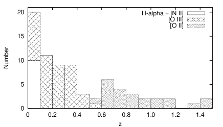
Figure 1: Histogram of the redshift distribution of the sources in our sample.

3 Observations and Data Reduction

3.1 Radio Observations

Arcsecond-scale resolution radio maps for the sample objects were obtained from a variety of sources (referenced in figure captions). Sources for which 5 or 8-GHz VLA ‘A’ array maps were not already available were reduced using archival data. The cleaning and self-calibration of the raw data was performed using the NRAO’s AIPS software package. We present new maps for the following sources: 3C124, 3C135, 3C284, 3C303.1, 3C341, 3C368, 3C379.1, and 3C382. Table 1 lists the observation parameters for the new VLA maps, including the date of observation, frequency and RMS noise of the final map.

3.2 Optical Observations

Snapshot images were taken using the LRFs on HST’s WFPC2 instrument. There are 3 WF chips and 1 PC chip. The chip on which the LRF images a target varies with the selected wavelength. We have noted the chip upon which a source was imaged in Table 2. Nearby objects ($z\lesssim 0.03$) were imaged in H$\alpha$+[NII]. Objects at intermediate redshifts were imaged in [OIII] 5007 $\AA$ and objects at high redshift ($z>0.5$) were imaged in [OII] 3727 $\AA$. Table 2 also lists which emission line was imaged for each source. All of the LRF observations consisted of a pair of 300 sec exposures taken in “snapshot” mode. The images were calibrated and combined using the CRREJ procedure to remove cosmic rays (Biretta 1996). Because the design of the LRF does not allow direct observations of the flat field, the images were flat fielded using the F656N flat. Note that due to the small size of the WFPC2 pixels, we are sensitive only to high surface brightness extended emission line gas.

In order to obtain images of only the emission line region (ELR), the continuum contribution to the LRF images was subtracted. This was usually done using an image of the object in the broadband F702W filter. The continuum was scaled to the observed wavelength by assuming a 3000K blackbody spectrum for the continuum (Biretta et al. 2002). In some cases the continuum was contaminated by emission lines. Baum et al. (1988) discussed the uncertainties in flux calibration due to contamination from emission lines. Using standard line ratios, they found corrections from 1.002 to 1.36 (median 1.09). We have not applied corrections for emission line contamination to our data, but the values given by them indicate the uncertainty due to contamination. Continuum images were not available for four sources, 3C98, 3C273, 3C289, and 3C323.1, and the subtraction could not be performed. These sources have been left out of the analysis, but their narrow-band LRF images are presented if the source was detected.

4 Optical Data Analysis

We grouped the emission-line nebulae into 4 broad optical morphological categories: ‘extended’ sources (21 sources), ‘partially extended’ sources (33 sources), slightly or unresolved sources (12 sources), and non-detections (11 sources). Four sources were eliminated due to the lack of a continuum image for subtraction. Sources were classified as extended if the 3-$\sigma$ contour was extended compared with the expected PSF in the continuum subtracted image. ‘Partially extended’ sources are those which feature extensions smaller than 2$\arcsec$ but do not match the PSF. They often resemble an unresolved source, with a small faint extension. We analyzed only the ‘extended’ and ‘partially extended’ sources, as we were able to determine reliable position angles and/or angular sizes for most of these objects. Table 3 lists the morphological categories for each object.

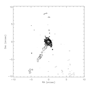
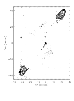
Figure 18: 3C109 (Radio/Optical Overlay) - Radio is shown in contours. Optical is shown in grey scale. Left: Closeup of the core. Right: View of the overall radio source. Radio levels are (0.199, 0.281, 0.398, 0.563, 0.796, 1.125, 1.591, 2.250, 3.182, 4.501, 6.365, 9.001, 12.730, 18.002, 25.459, 36.005, 50.918, 72.009, 101.837, 144.019) mJy. Optical levels are (46.7, 66.0, 93.3, 132.0, 186.7, 264.0, 373.4, 528.0, 749.8) * $10^{-14}$ erg $s^{-1}$ $cm^{-2}$. Both images have the same levels.

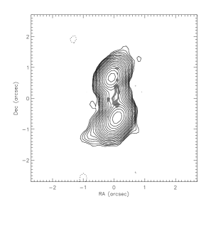
Figure 20: 3C124 (Radio/Optical Overlay) - Radio is shown in contours. Optical is shown in grey scale. Radio levels are (0.182, 0.258, 0.365, 0.516, 0.730, 1.032, 1.459, 2.064, 2.918, 4.127, 5.837) mJy. Optical levels are (64.6, 91.4) * $10^{-14}$ erg $s^{-1}$ $cm^{-2}$.

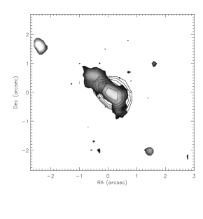
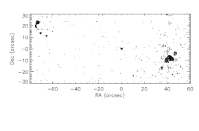
Figure 22: 3C135 (Radio/Optical Overlay) - Radio is shown in contours. Optical is shown in grey scale. Left: Closeup of the core. Right: View of the overall radio source. Radio levels are (0.151, 0.214, 0.303, 0.429, 0.606, 0.857, 1.212, 1.714, 2.424, 3.428, 4.848, 6.856) mJy. Optical levels are (96.0, 135.9, 192.2, 271.8, 384.3, 543.5, 768.6, 1087.0, 1537.3, 2174.0) * $10^{-14}$ erg $s^{-1}$ $cm^{-2}$. Both images have the same levels.

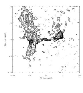
Figure 24: 3C171 (Radio/Optical Overlay) - Radio is shown in contours. Optical is shown in grey scale. Radio levels are (0.164, 0.231, 0.327, 0.463, 0.654, 0.925, 1.309, 1.851, 2.618, 3.702, 5.235, 7.404, 10.470, 14.807, 20.941, 29.615, 41.882, 59.230, 83.763) mJy. Optical levels are (52.4, 74.0, 104.7, 148.1, 209.4, 296.2, 418.9, 592.4, 837.7, 1184.7, 1675.4, 2369.4) * $10^{-14}$ erg $s^{-1}$ $cm^{-2}$. The radio map courtesy of David Floyd (private communication).

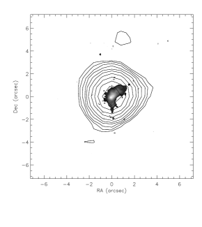
Figure 26: 3C223 (Radio/Optical Overlay) - Radio is shown in contours. Optical is shown in grey scale. Left: Closeup of the core. Right: View of the overall radio source. Radio levels are (0.258, 0.365, 0.516, 0.730, 1.032, 1.459, 2.064, 2.919, 4.128, 5.838, 8.256) mJy. Optical levels are (100.8, 142.6, 201.7, 285.2, 403.3, 570.4, 806.7, 1140.8, 1613.3, 2281.6, 3226.7, 4563.3, 6453.5) * $10^{-14}$ erg $s^{-1}$ $cm^{-2}$. Both images have the same levels. The radio map courtesy of David Floyd (private communication).

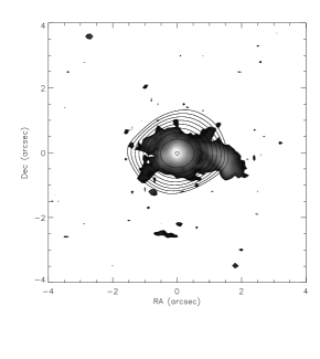
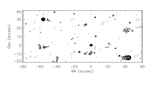
Figure 28: 3C234 (Radio/Optical Overlay) - Radio is shown in contours. Optical is shown in grey scale. Left: Closeup of the core. Right: View of the overall radio source. Radio levels are (2.226, 3.148, 4.451, 6.295, 8.903, 12.590, 17.806, 25.181, 35.611, 50.362, 71.222, 100.724, 142.445, 201.447, 284.890, 402.895, 569.779) mJy. Optical levels are (134.6, 190.4, 269.3, 380.8, 538.6, 761.7, 1077.1, 1523.3, 2154.3, 3046.6, 4308.6, 6093.3, 8617.2, 12186.6, 17234.5, 24373.2, 34468.9) * $10^{-14}$ erg $s^{-1}$ $cm^{-2}$. Both images have the same levels. Radio map from Neff et al. (1995).

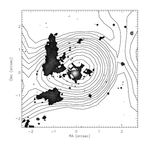
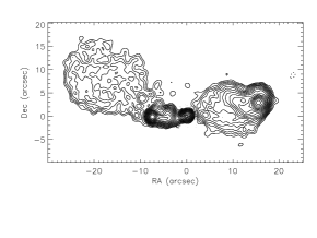
Figure 30: 3C249.1 (Radio/Optical Overlay) - Radio is shown in contours. Optical is shown in grey scale. Left: Closeup of the core. Right: View of the overall radio source. Radio levels are (0.674, 0.953, 1.348, 1.907, 2.696, 3.813, 5.393, 7.627, 10.786, 15.253, 21.571, 30.506, 43.142, 61.013, 86.285, 122.025, 172.570, 244.050) mJy. Optical levels are (184.0, 260.2, 368.0, 520.4, 735.9, 1040.7, 1471.9, 2081.5, 2943.7, 4163.0, 33304.3, 47099.4, 66608.6, 94198.7) * $10^{-14}$ erg $s^{-1}$ $cm^{-2}$. Both images have the same levels. Radio map from J. P. Laing (Image obtained from the 3CRR Atlas (http://www.jb.man.ac.uk/atlas).).

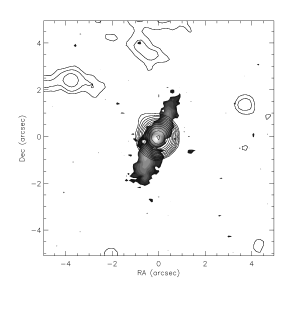
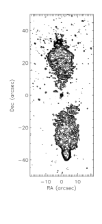
Figure 54: 3C381 (Radio/Optical Overlay) - Radio is shown in contours. Optical is shown in grey scale. Left: Closeup of the core. Right: View of the overall radio source. Radio levels are (0.102, 0.144, 0.203, 0.288, 0.407, 0.575, 0.814, 1.151, 1.627, 2.301, 3.254, 4.602, 6.509, 9.205, 13.018, 18.410, 26.035, 36.819, 52.070, 73.639) mJy. Optical levels are (87.8, 124.2, 175.7, 248.4, 351.4, 496.9, 702.7, 993.8, 1405.5, 1987.6, 2811.0) * $10^{-14}$ erg $s^{-1}$ $cm^{-2}$. Both images have the same levels. The radio map was provided by David Floyd (Private Communication).

To examine the spatial coincidence of the ELR and the radio source, the radio and optical images for the ‘extended’ sources were combined into overlays. In general, the images were registered using the radio core (for the radio sources), and the centroid of the host galaxy (obtained from the continuum images). One ‘extended’ source (3C305) has a known dust lane, making centroiding on the continuum image unreliable. We attempted to determine a center through ellipse fitting to the outer portion of the galaxy, but this was unsuccessful due to the close companion galaxy. The registration in the image presented was done using centroiding on the continuum image. The overlays are shown in Figures 10 - 54 along with the continuum and emission-line images for each source.

Position angles (PAs) for the ‘extended’ sources were measured using the emission within the 3-$\sigma$ contour, with the PA passing through the nucleus of the host galaxy in the direction of the longest extent of the emission line nebulae. PAs for the partially extended sources were determined using IRAF’s ‘ellipse’ task. Radio PAs were taken from the literature (if available), or measured from hotspot-to-hotspot for FRIIs or across the longest extent for FRIs on the radio maps. The measurement of the difference in the PAs is independent of the spatial alignment of the radio and optical images as the position angles are independently determined from the images.

A measure of alignment between the ELR and the radio source was determined by taking the absolute value of the difference in position angles of the radio source and the ELR. If $\Delta$PA $\leqslant$ 30 degrees, the ELR and radio source were considered aligned. In some cases the ELR displayed a position angle for the inner regions which differed from the large scale position angle. In most cases, the usage of an “inner PA” did not cause misaligned objects to be moved into the aligned category, so only the large-scale PA was used for the purposes of our analysis.

Emission line fluxes were measured using IRAF’s ‘apphot’ set of tasks. Luminosities and sizes were calculated using a cosmology of H₀=71 km s^-1, $\Omega$_M=0.27, and $\Omega$_vac=0.73. Values were obtained using an online cosmology calculator (Wright 2006). In order to compare the luminosities from each source, the measured fluxes were converted to H$\alpha$ fluxes using line ratios derived from observations of narrow-line radio galaxies (Koski 1978). The ratios of [OIII], [OII], and H$\alpha$+[NII] to H$\alpha$ were 3, 1.23, and 2.08 respectively.

5 Properties of the Nebulae

Here we discuss the properties of the nebulae and their relationship to the radio source. Individual source descriptions are provided in Appendix A. In Table 4 we provide morphological information about the radio structure, including classifications, position angles, and angular sizes. We also present luminosities for each source. Table 3 contains the morphological information for the continuum-subtracted emission line images. This includes position angles, angular sizes, and fluxes. In addition, this table contains the V-band magnitudes for the host galaxies and the position angle of the galaxy.

The detection statistics varied depending on the emission line observed. Nine of ten sources (90%) imaged in H$\alpha$+[NII] were detected. Forty-three of forty-seven sources (91%) imaged in [OIII] were detected, while fifteen of twenty-three (65%) [OII] detections were made.

The statistical significance of the observed relationships discussed in this section are given in Table 5. The Kendall tau value is a measure of the correlation between the specified measurements. The Spearman’s rho value is a similar measure, describing how likely the two measurements are to increase or decrease concordantly. Statistical values for non-correlations are given in Table 6.

5.1 Alignment Effect

We find that 19 of 37 sources for which a PA could be measured showed alignment between the high surface brightness ELR and the radio source to within 30 degrees (Figure 2). We have 4 sources at $z>0.6$ which all show strong alignment. In the remaining 33 sources at $z<0.6$, 15 show alignment. The median values of the position angle difference in bins of redshift do not decrease significantly as a function of $z$ out to 0.6. However, the upper envelope of the position angle differences does seem to decrease with redshift. We clearly see a weaker alignment effect at low redshift than is seen at the high redshifts $z>0.6$. Our high resolution HST data show that the lack of strong alignment at $z<0.6$ is not due to a lack of spatial resolution.

Figure 2: Relative alignment of the radio source and ELR as a function of redshift. No correlation was present with the Kendall tau test giving a non-correlation probability of 0.0913 and Spearman’s rho test giving a probability of 0.1540 of a correlation not being present.

We investigated the possibility of the misaligned objects being predominantly broad line radio galaxies (BLRGs). According to the unified scheme (Urry & Padovani 1995), BLRGs are not expected to show alignment as the jet would be pointing almost along the line of sight. However, BLRGs make up only 11 of the sources with measured position angle differences, and several of the BLRGS show alignment (3C234, 3C268.3, 3C277.1). Thus, orientation of the radio jet close to the line of sight is not responsible for the misalignment at $z<0.6$.

A potential concern is that much of the low redshift observations ($0.03<z<0.5$) are obtained using the [OIII] line which is higher ionization than the [OII] and H$\alpha$+[NII]. If the high ionization gas has very different morphology and position angle than the lower excitation gas, this might reduce the strength of the alignment at low redshift. However, observations of radio galaxies in which both [OII] and [OIII] are obtained show that the estimated large scale position angles are consistent (e.g. Tilak et al. 2005).

Another possible bias is the extent of the ELRs for different emission lines. Studies of single objects in multiple emission lines indicate typical ratios in the extended emission of $\sim$1 - 6 for [O III]/[O II] and $\sim$1 - 4 for [O III]/H$\alpha$ (e.g. Tilak et al. 2005; Solórzano-Iñarrea & Tadhunter 2003; Robinson et al. 2000). Thus, as the transition between lines is made, the ELR should be smaller for [O II] than for [O III]. As will be discussed in $\S$ 5.3, the opposite is found.

Over the redshift range of our sample (0.017 $\leqslant z\leqslant$ 1.406), the expected (1+z)⁴ dimming of surface brightness is a factor of $\sim$30 - though the details will depend on the actual surface brightness profiles. Thus, both the transition from [OIII] to [OII] and the (1+z)⁴ effect should result in apparently smaller ELR at higher redshift. Despite this, we see emission line size increasing with redshift (see $\S$ 5.3), suggesting that this result is real.

In order to investigate the possible effect of an instrumental sensitivity selection effect on the detection of alignment, we redshifted the faintest level in the emission line images to see what would be detected if located at $z=0.5$ (just prior to the onset of strong alignment). None of the misaligned sources showed any alignment when viewed using these modified levels. This indicates that the alignment effect is not due to a selection effect of the sensitivity of the instrument, but rather to some other inherent attribute of the source and its environment.

5.1.1 Comparison with Ground Based Data

Figure 3: Top Left: Comparison of the HST luminosities from our data with ground based data from previous studies (Baum & Heckman 1989; McCarthy et al. 1995). The HST luminosities are much lower due to the lower surface brightness sensitivity of WFPC2. Top Right: Comparison of the angular sizes in our HST data with ground based data. The extended emission is of low surface brightness and we do not detect the full extent of the ELR as seen from the ground. Bottom Left: A comparison of the Delta PA derived from the HST data and ground based data. While many of the values are quite similar, some are significantly different. The line in all plots is y=x.

The emission line images from HST were compared with previous studies using ground based imaging (Figure 3). Morphologies and position angles were generally consistent between the two sets consistent with the hypothesis that the nebulae position angles do not exhibit large changes in position angle as a function of size scale. However, because of the lower surface brightness sensitivity of the HST/WFPC2 camera, the HST images show only the brighter inner regions of the nebulae. Thus, the HST measured sizes and emission line fluxes tend to be smaller than those measured on ground based images.

Figure 4 shows a comparison of the distribution of position angle differences from ground-based data (Baum et al. 1988; Rigler et al. 1992; McCarthy et al. 1995) with our HST data. There is a suggestion that the HST data shows an alignment effect which is weaker than seen in the ground-based data at the same redshifts. The Kolmogorov-Smirnov (KS) test indicates that the distribution of position angle differences in the HST data is consistent with a uniform distribution of angles, while the ground based data are not (see Table 7). If larger samples confirm this result, this may be due to the HST data mainly being sensitive to the higher surface brightness, more compact emission, suggesting that the alignment effect is mainly produced in fainter, more extended emission line gas.

Figure 4: These figures show histograms of relative alignment between the emission line region and the radio source for various redshift ranges. The left column plots ground-based data compiled in McCarthy et al. (1995) while the right column shows our HST/WFPC2 data. The top two plots are for $z<0.1$. The middle row is for $0.3<z<0.6$ and the bottom row is for $0.1<z<0.6$.

5.2 Relative Sizes of the Emission Line Region and the Radio Source

We computed the ‘size ratio’ comparing the relative projected linear sizes of the radio source and the high surface brightness emission line region. The linear sizes for FR II and CSS sources were measured from hotspot to hotspot, and the linear sizes for FR I sources were measured across the overall extent. Linear sizes for the emission line regions were measured roughly along the long axis (if such an axis existed). Comparing the relative sizes of the radio source and ELR with the relative alignment indicates that sources with similar radio and ELR sizes are more frequently aligned than sources in which the ELR is much smaller than the radio source (Figure 5). This is true at all redshifts (Figure 5). We also note that all six of the small sources (D $<$ 15 kpc, i.e., CSS) are well aligned (Figure 6). All six of these have size ratios between $\sim$0.3 and $\sim$ 6. These results suggest that the alignment at low redshift results when the source is smaller/younger and of a similar size as the nebula. This is consistent with suggestions that the alignment is due to mechanical energy input from the radio source (e.g., de Vries et al. 1999; Axon et al. 2000; Best et al. 2000; Inskip et al. 2002a, b). At low redshifts, suitable gas clouds are likely to exist only on the scale of the host galaxy.

Figure 5: Left: Plot of the calculated size ratio between the radio source and the emission line region as a function of alignment between the two. The sources with size ratios of roughly one have optical morphologies which are closely aligned with the radio source. Both Kendall tau and Spearman’s rho tests indicate the presence of a correlation with non-correlation probabilities of 0.0001 and 0.0003 respectively. Right: Size ratio as a function of $z$. The sources with size ratios near unity are found at both high and low redshifts.

In addition, 13 of the 29 large sources (size greater than 50 kpc) also show alignment to within 30^∘. These sources are much bigger than their emission line nebulae (factors of 10-100). Some of this alignment may be produced by chance if the position angles differences in at least some low $z$ sources are randomly distributed. However, some of the alignment may be real since we suspect the effect is starting to turn on at these redshifts. Diagnostic line ratios and kinematics indicate that shocks are important when the radio source size is comparable to the aligned emission line nebula size and that photoionization dominates when the radio source is much larger than the nebula (e.g., Best et al. 2000; Inskip et al. 2002a; Moy & Rocca-Volmerange 2002; O’Dea et al. 2002; Labiano et al. 2005). Thus, in these large sources, the alignment may be produced by photoionization from the central AGN along the “ionization cone”. Recombination times for warm gas (T $\sim$10⁴ K) are roughly 10³ years (Osterbrock 1989) while the lifetimes of the radio sources are roughly 10⁷ – 10⁸ years, indicating the ionizing mechanism must be on-going throughout the lifetime of the source.

Figure 6: Plot of the projected radio size as a function of the relative alignment between the radio source and the emission line nebulae. All of the small sources are aligned while only some of the large sources are aligned.

5.3 Emission Line Nebula Size and Luminosity

The size of the high surface brightness ELR increases with increasing radio power (Figure 7) and/or with increasing redshift (Figure 8). Both correlations are somewhat weaker for just the $z<0.6$ objects. At higher redshifts, dense gas clouds are found on increasingly larger scales culminating in the large Ly-$\alpha$ halos surrounding powerful radio galaxies ( van Ojik et al.1997; Reuland et al. 2003). Of course, the radio luminosity will also increase with redshift in flux density limited samples, meaning the correlations may be related. Studies which attempt to break the redshift-radio power degeneracy suggest that the alignment depends on both redshift and radio power (e.g., Inskip et al. 2002b). The more powerful radio sources can provide both more mechanical energy and more ionizing photons (Baum & Heckman 1989; Rawlings & Saunders 1991). Thus both the presence of gas on larger scales as well as the larger energy input from the radio source could result in the emission line size increasing with redshift and radio power.

Figure 7: Plot of projected emission line nebulae size against logarithm of the radio luminosity. The probabilities of this being a non-correlation are 0.0039 (Kendall tau) and 0.0067 (Spearman’s rho) for the whole sample and are 0.0119 (Kendall tau) and 0.0172 (Spearman’s rho) for $z<0.6$.

Figure 8: Plot of the projected emission line nebulae size as a function of redshift. The probabilities of this being a non-correlation are 0.0050 (Kendall tau) and 0.0055 (Spearman’s rho) for the whole sample and are 0.0152 (Kendall tau) and 0.0136 (Spearman’s rho) for $z<0.6$.

Comparing the luminosity of the ELR with the relative alignment (Figure 9) indicates aligned sources have more luminous ELRs. The correlation becomes weaker for the redshift range $z<0.6$. We find that the correlation is further weakened if we also exclude $z<0.1$ (Figure 9). The existence of the (weak) correlation at $z<0.6$ suggests that the radio source provides additional energy to the emission line gas along the direction of the radio axis and thus, there is a ‘real’ though weak alignment effect at these low redshifts.

Figure 9: Left: Plot of logarithm of the emission line nebulae luminosity against the relative alignment between the radio source and the emission line nebulae. The probabilities of this being a non-correlation are 0.0083 (Kendall tau) and 0.0134 (Spearman’s rho) for the whole sample and are 0.0356 (Kendall tau) and 0.0473 (Spearman’s rho) for $z<0.6$. Right: Same plot as that on the left, but for sources with $0.1<z<0.6$ only. The probability of this being a non-correlation is 0.0429 (Kendall tau).

6 Conclusions

We present WFPC2 LRF images of selected emission lines in a sample of 3CR radio galaxies with bright emission lines. We detect clumpy, high surface brightness emission line gas with a wide range of morphologies. We examine the properties of the emission line gas and its relationship to the radio source, and in particular the nature of the alignment effect at $z<0.6$ where the effect is beginning to become important.

We find there is a weak alignment effect in our low $z$ sample ($z<0.6$). The effect is clearly weaker than seen at high redshifts and is also somewhat weaker than seen at similar redshifts in ground-based data. This suggests that the alignment effect is dominated by the more extended lower surface brightness emission line gas which falls below our detection threshold in WFPC2.

The alignment at low redshift is strong when the radio source and the nebula are both of order galactic scales (e.g., CSS sources). This implies there is mechanical energy input from the radio source as it propagates through the ambient gas in the host galaxy (e.g., de Vries et al. 1999; Axon et al. 2000).

There is a weak trend for the nebulae in the aligned sources (at all radio/optical size ratios) to have higher line luminosity. This suggests that the radio source preferentially provides energy to gas which is along the radio source axis. This is likely to be predominantly mechanical energy when the radio source and nebulae have similar sizes, and predominantly photoionization when the radio source is much larger than the nebula (e.g., Best et al. 2000; Inskip et al. 2002a; Moy & Rocca-Volmerange 2002; O’Dea et al. 2002; Labiano et al. 2005).

There is a weak trend for the size of the high surface brightness emission line nebulae to increase with increasing radio power and/or redshift over the range $z<0.6$. This may be due to both the increasing presence of gas on large scales and the ability of the more powerful radio sources to provide additional mechanical energy and/or ionizing photons as a function of redshift.

Thus, there is evidence for a modest excess of aligned sources at low redshift ($z<0.6$). The alignment is strong when the radio source and emission line nebula are both on galactic scales. There are also weak trends for the aligned emission line nebulae to be more luminous, and for the emission line size to increase with redshift and radio power. The combination of these results suggests that there is a limited but real capacity for the radio source to influence the properties of the emission line nebulae at these low redshifts.

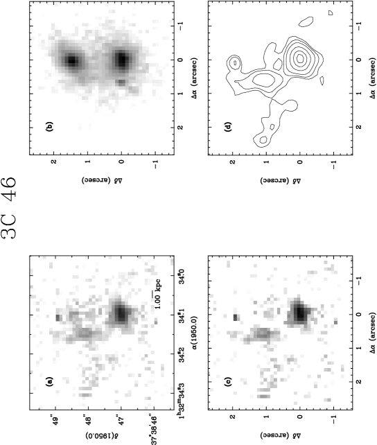
Figure 10: 3C46 (Optical Montage) - Starting at the upper left, going clockwise: LRF Image; Broadband Image; Continuum Subtracted image [Contours]; Continuum Subtracted Image [Grey scale]

Figure 11: 3C46 (Radio/Optical Overlay) - Radio is shown in contours. Optical is shown in grey scale. Left: Closeup of the core. Right: View of the overall radio source. Radio levels are (1.215, 1.719, 2.431, 3.437, 4.861, 6.875, 9.722, 13.750, 19.445, 27.499) mJy. Optical levels are (56.5, 79.9, 113.0, 159.9, 159.9, 226.1, 319.7, 452.2, 639.5) * $10^{-14}$ erg $s^{-1}$ $cm^{-2}$. Both images have the same levels. Radio map from Neff et al. (1995).

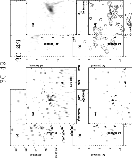
Figure 12: 3C49 (Optical Montage) - Starting at the upper left, going clockwise: LRF Image; Broadband Image; Continuum Subtracted image [Contours]; Continuum Subtracted Image [Grey scale]

Figure 13: 3C49 (Radio/Optical Overlay) - Radio is shown in contours. Optical is shown in grey scale. Radio levels are (3.555, 5.028, 7.110, 10.055, 14.220, 20.110, 28.440, 40.220, 56.880, 80.440, 113.760, 160.881, 227.520, 321.762, 455.040) mJy. Optical levels are (18.2, 25.7, 33.3) * $10^{-14}$ erg $s^{-1}$ $cm^{-2}$ The radio map is from Neff et al. (1995).

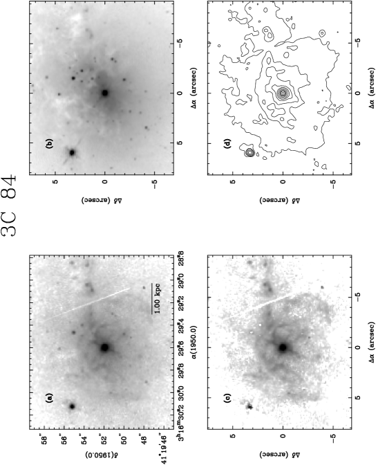
Figure 14: 3C84(Optical Montage) - Starting at the upper left, going clockwise: LRF Image; Broadband Image; Continuum Subtracted image [Contours]; Continuum Subtracted Image [Grey scale]

Figure 15: 3C84 (Emission Line Only) - Optical is shown in grey scale. Optical levels are (48.6, 68.7, 97.1, 137.3, 194.2, 274.7, 388.5, 549.4, 777.0, 1098.8, 1553.9, 2197.6, 3108.0, 4395.2, 6215.8, 8790.4) * $10^{-14}$ erg $s^{-1}$ $cm^{-2}$ (Note: In Radio maps 3C84 is highly core dominated. A worthwhile 5 or 8 GHz radio map could not be located, so only the emission line image is presented.)

Figure 16: 3C98 (Narrow band Image) - This is the narrow-band optical (LRF) image. The levels are (44.5, 62.9, 89.0, 125.8, 177.9, 251.6, 355.8, 503.2, 711.7, 1006.5, 1423.4, 2012.9) $10^{-14}$ erg $s^{-1}$ $cm^{-2}$.

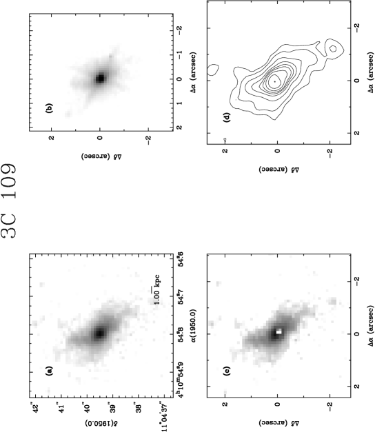
Figure 17: 3C109(Optical Montage) - Starting at the upper left, going clockwise: LRF Image; Broadband Image; Continuum Subtracted image [Contours]; Continuum Subtracted Image [Grey scale]

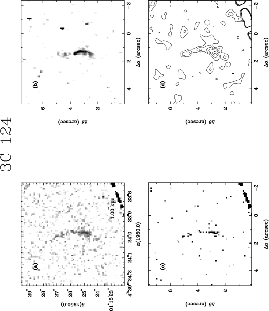
Figure 19: 3C124 (Optical Montage) - Starting at the upper left, going clockwise: LRF Image; Broadband Image; Continuum Subtracted image [Contours]; Continuum Subtracted Image [Grey scale]

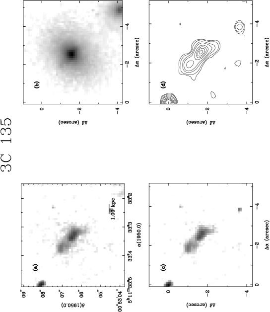
Figure 21: 3C135 (Optical Montage) - Starting at the upper left, going clockwise: LRF Image; Broadband Image; Continuum Subtracted image [Contours]; Continuum Subtracted Image [Grey scale]

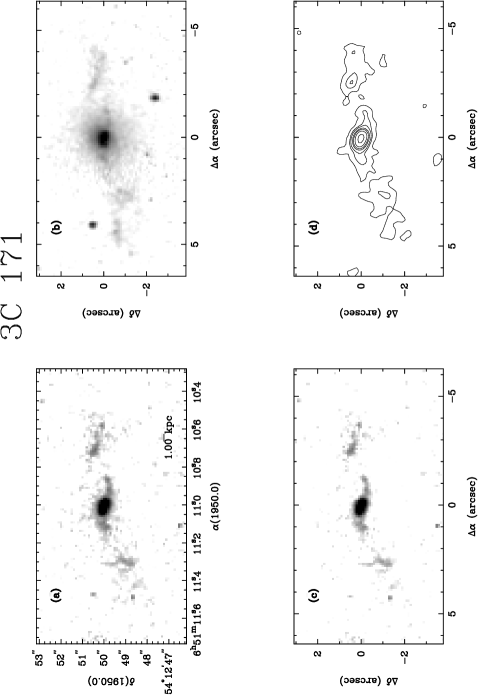
Figure 23: 3C171 (Optical Montage) - Starting at the upper left, going clockwise: LRF Image; Broadband Image; Continuum Subtracted image [Contours]; Continuum Subtracted Image [Grey scale]

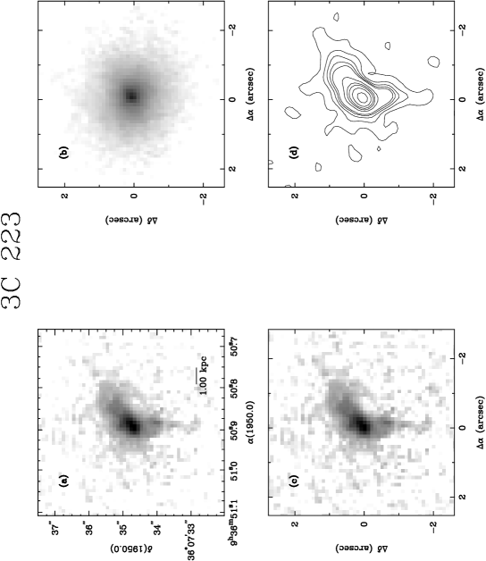
Figure 25: 3C223 (Optical Montage) - Starting at the upper left, going clockwise: LRF Image; Broadband Image; Continuum Subtracted image [Contours]; Continuum Subtracted Image [Grey scale]

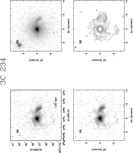
Figure 27: 3C234 (Optical Montage) - Starting at the upper left, going clockwise: LRF Image; Broadband Image; Continuum Subtracted image [Contours]; Continuum Subtracted Image [Grey scale]

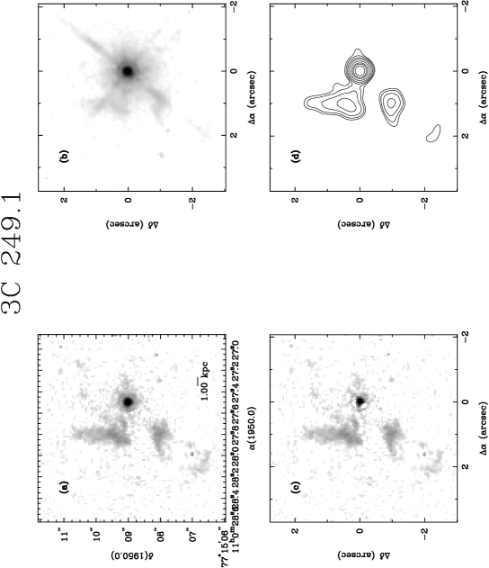
Figure 29: 3C249.1 (Optical Montage) - Starting at the upper left, going clockwise: LRF Image; Broadband Image; Continuum Subtracted image [Contours]; Continuum Subtracted Image [Grey scale]

Figure 31: 3C268.2 (Optical Montage) - Starting at the upper left, going clockwise: LRF Image; Broadband Image; Continuum Subtracted image [Contours]; Continuum Subtracted Image [Grey scale]

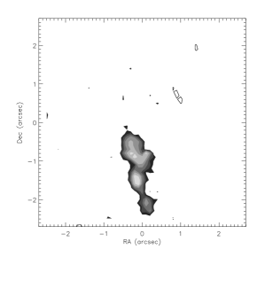
Figure 32: 3C268.2 (Radio/Optical Overlay) - Radio is shown in contours. Optical is shown in grey scale. Left: Closeup of the core. Right: View of the overall radio source. Radio levels are (1.212, 1.714, 2.424, 3.428, 4.848, 6.856, 9.696, 13.712) mJy. Optical levels are (62.8, 88.8, 125.6, 177.6, 251.2, 355.2, 502.3) * $10^{-14}$ erg $s^{-1}$ $cm^{-2}$. Both images have the same levels. The radio map is from Neff et al. (1995).

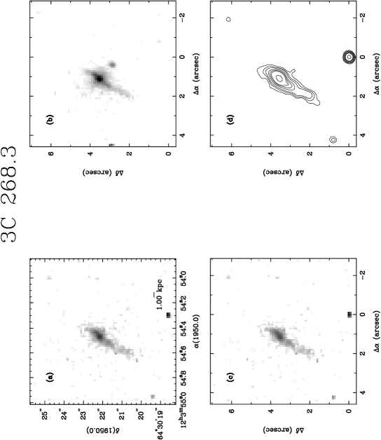
Figure 33: 3C268.3 (Optical Montage) - Starting at the upper left, going clockwise: LRF Image; Broadband Image; Continuum Subtracted image [Contours]; Continuum Subtracted Image [Grey scale]

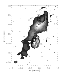
Figure 34: 3C268.3 (Radio/Optical Overlay) - Radio is shown in contours. Optical is shown in grey scale. Radio levels are (0.193, 0.272, 0.385, 0.545, 0.770, 1.090, 1.541, 2.179, 3.082, 4.358, 6.163, 8.716, 12.326, 17.432, 24.653, 34.864, 49.306, 69.729, 98.611, 139.457) mJy. Optical levels are (51.9, 73.4, 103.9, 146.9, 207.7, 293.8, 415.4) * $10^{-14}$ erg $s^{-1}$ $cm^{-2}$. The radio map is from Ludke et al. (1998).

Figure 35: 3C273 (Narrow band Image). Optical levels are (110.8, 156.6, 221.5, 313.3, 443.0, 626.6, 886.1, 1253.1, 1772.2, 2506.3, 3544.4, 5012.5, 7088.8, 10025.0, 14177.5, 20050.1 28355.1, 40100.2, 56710.2, 80200.4) * $10^{-14}$ erg $s^{-1}$ $cm^{-2}$.

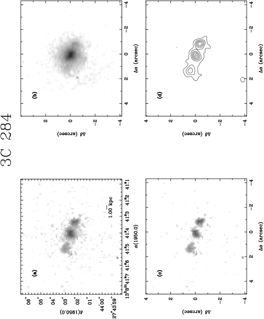
Figure 36: 3C284 (Optical Montage) - Starting at the upper left, going clockwise: LRF Image; Broadband Image; Continuum Subtracted image [Contours]; Continuum Subtracted Image [Grey scale]

Figure 37: 3C284 (Radio/Optical Overlay) - Radio is shown in contours. Optical is shown in grey scale. Left: Closeup of the core. Right: View of the overall radio source. Radio levels are (1.796, 2.540, 3.593, 5.081, 7.186, 10.162, 14.371, 20.324, 28.742) mJy. Optical levels are (49.1, 69.5, 98.3, 139.0, 196.5, 277.9, 393.0) * $10^{-14}$ erg $s^{-1}$ $cm^{-2}$. Both images have the same levels.

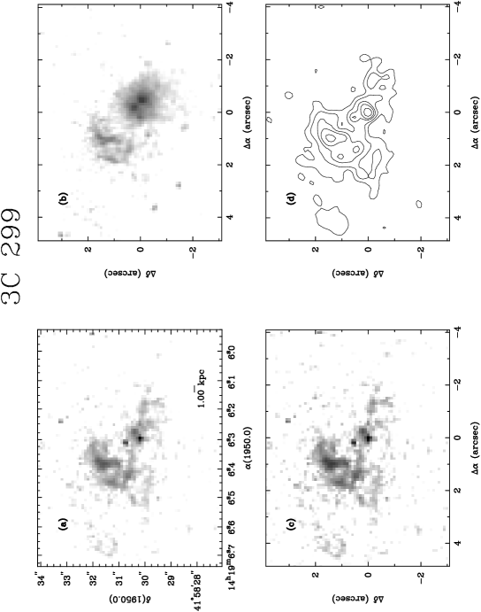
Figure 38: 3C299(Optical Montage) - Starting at the upper left, going clockwise: LRF Image; Broadband Image; Continuum Subtracted image [Contours]; Continuum Subtracted Image [Grey scale]

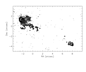
Figure 39: 3C299 (Radio/Optical Overlay) - Radio is shown in contours. Optical is shown in grey scale. Radio levels are (0.430, 0.608, 0.860, 1.216, 1.720, 2.432, 3.439, 4.864, 6.878, 9.728, 13.757, 19.455, 27.514, 38.910, 55.027, 77.820, 110.054, 155.640, 220.109, 311.281) mJy. Optical levels are (52.6, 74.3, 105.1, 148.7, 210.3, 297.4, 420.6, 594.8, 841.1, 1189.5, 1682.3) * $10^{-14}$ erg $s^{-1}$ $cm^{-2}$. The radio map was provided by J. P. Laing (Image obtained from the 3CRR Atlas (http://www.jb.man.ac.uk/atlas).).

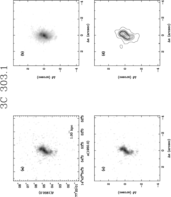
Figure 40: 3C303.1 (Optical Montage) - Starting at the upper left, going clockwise: LRF Image; Broadband Image; Continuum Subtracted image [Contours]; Continuum Subtracted Image [Grey scale]

Figure 41: 3C303.1 (Radio/Optical Overlay) - Radio is shown in contours. Optical is shown in grey scale. Radio levels are (0.228, 0.322, 0.455, 0.644, 0.910, 1.288, 1.821, 2.575, 3.642, 5.150, 7.283, 10.300, 14.566, 20.600, 29.133, 41.200, 58.266, 82.400, 116.531) mJy. Optical levels are (46.3, 65.5, 92.5, 130.9, 185.2, 261.9, 370.3, 523.7, 740.7, 1047.4, 1481.3) * $10^{-14}$ erg $s^{-1}$ $cm^{-2}$.

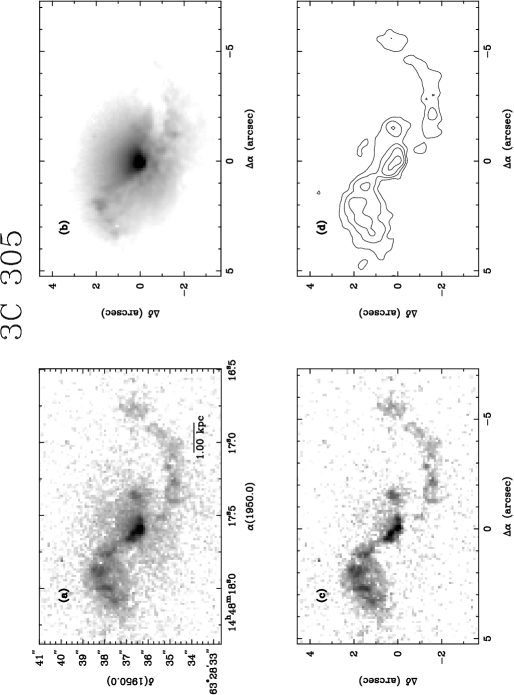
Figure 42: 3C305 (Optical Montage) - Starting at the upper left, going clockwise: LRF Image; Broadband Image; Continuum Subtracted image [Contours]; Continuum Subtracted Image [Grey scale]

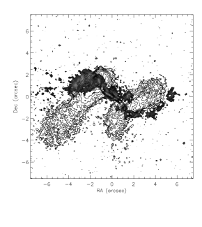
Figure 43: 3C305 (Radio/Optical Overlay) - Radio is shown in contours. Optical is shown in grey scale. Radio levels are (0.236, 0.334, 0.473, 0.669, 0.946, 1.337, 1.891, 2.675, 3.782, 5.349, 7.565, 10.698, 15.130, 21.396, 30.259, 42.793, 60.518, 85.586) mJy. Optical levels are (166.3, 235.2, 332.6, 470.4, 665.3, 940.9, 1330.6, 1881.7, 2661.2, 3763.5, 5322.4) * $10^{-14}$ erg $s^{-1}$ $cm^{-2}$. The radio map was provided by J. P. Laing (Image obtained from the 3CRR Atlas (http://www.jb.man.ac.uk/atlas)).

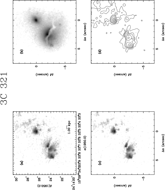
Figure 44: 3C321 (Optical Montage) - Starting at the upper left, going clockwise: LRF Image; Broadband Image; Continuum Subtracted image [Contours]; Continuum Subtracted Image [Grey scale]

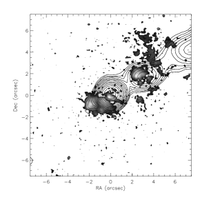
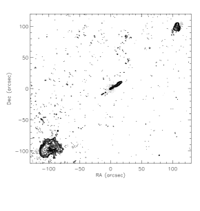
Figure 45: 3C321 (Radio/Optical Overlay) - Radio is shown in contours. Optical is shown in grey scale. Left: Closeup of the core. Right: view of the overall radio source. Radio levels are (0.368, 0.520, 0.736, 1.040, 1.471, 2.081, 2.942, 4.161, 5.885, 8.322, 11.770, 16.645, 23.539, 33.289, 47.078, 66.579, 94.157, 133.158, 188.314, 266.316) mJy. Optical levels are (81.0, 114.5, 162.0, 229.1, 232.9, 458.1, 647.9, 916.3, 1295.8, 1832.6, 2591.6, 3665.1) * $10^{-14}$ erg $s^{-1}$ $cm^{-2}$. Both images have the same levels. The radio map was provided courtesy of David Floyd (private communication).

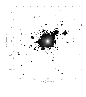
Figure 46: 3C323.1 (Narrow band Image) - Optical levels are (94.1, 133.0, 188.1, 266.1, 376.3, 532.2, 752.6, 1064.3, 1505.2, 2128.6, 3010.4, 4257.3, 6020.7, 8514.6, 12041.4, 17029.2, 24082.9, 34058.3, 48165.8, 68116.7) * $10^{-14}$ erg $s^{-1}$ $cm^{-2}$.

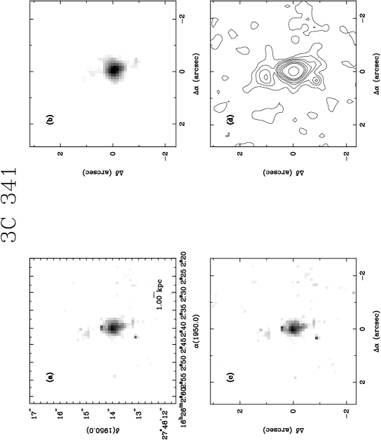
Figure 47: 3C341 (Optical Montage) - Starting at the upper left, going clockwise: LRF Image; Broadband Image; Continuum Subtracted image [Contours]; Continuum Subtracted Image [Grey scale]

Figure 48: 3C341 (Radio/Optical Overlay) - Radio is shown in contours. Optical is shown in grey scale. Left: Closeup of the core. Right: View of the overall radio source. Radio levels are (0.288, 0.407, 0.576, 0.815, 1.152, 1.629, 2.304, 3.258, 4.608, 6.517, 9.216, 13.033) mJy. Optical levels are (58.0, 82.0, 115.9, 163.9, 231.9, 327.9, 463.7, 655.8) * $10^{-14}$ erg $s^{-1}$ $cm^{-2}$. Both images have the same levels.

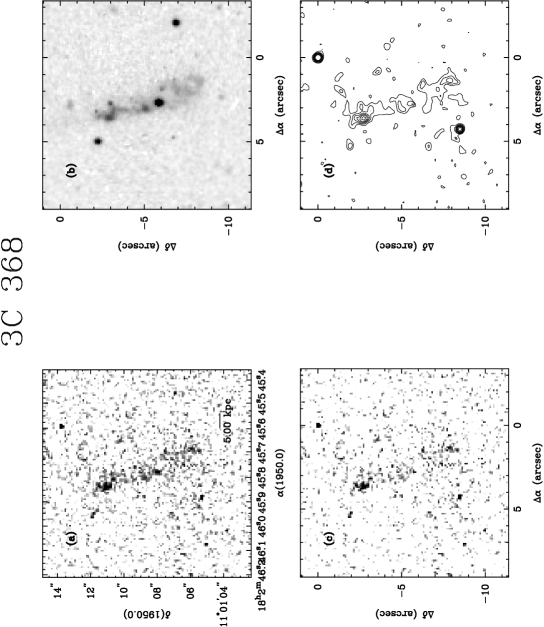
Figure 49: 3C368 (Optical Montage) - Starting at the upper left, going clockwise: LRF Image; Broadband Image; Continuum Subtracted image [Contours]; Continuum Subtracted Image [Grey scale]

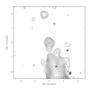
Figure 50: 3C368 (Radio/Optical Overlay) - Radio is shown in contours. Optical is shown in grey scale. Left: Closeup of the core. Right: View of the overall radio source. Radio levels are (0.098, 0.138, 0.195, 0.276, 0.391, 0.553, 0.782, 1.105, 1.563, 2.211, 3.126, 4.421, 6.253, 8.843, 12.506, 17.686, 25.011, 35.371) mJy. Optical levels are (68.7, 97.2, 137.5) * $10^{-14}$ erg $s^{-1}$ $cm^{-2}$. Both images have the same levels.

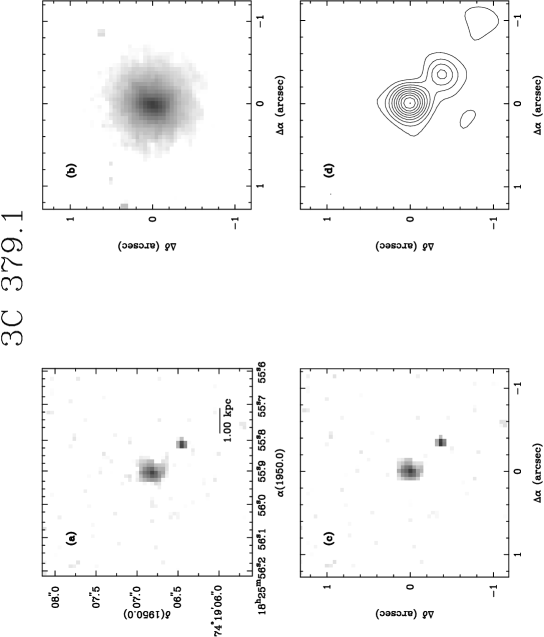
Figure 51: 3C379.1 (Optical Montage) - Starting at the upper left, going clockwise: LRF Image; Broadband Image; Continuum Subtracted image [Contours]; Continuum Subtracted Image [Grey scale]

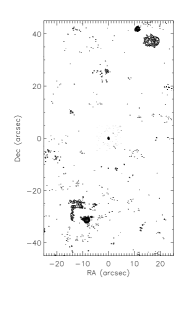
Figure 52: 3C379.1 (Radio/Optical Overlay) - Radio is shown in contours. Optical is shown in grey scale. Left: Closeup of the core. Right: View of the overall radio source. Radio levels are (0.225, 0.318, 0.449, 0.635, 0.898, 1.271, 1.797, 2.541, 3.594, 5.082, 7.187, 10.164, 14.374, 20.328) mJy. Optical levels are (186.8, 264.2, 373.7, 528.4, 747.3, 1056.9) * $10^{-14}$ erg $s^{-1}$ $cm^{-2}$. Both images have the same levels.

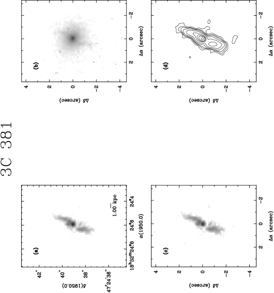
Figure 53: 3C381 (Optical Montage) - Starting at the upper left, going clockwise: LRF Image; Broadband Image; Continuum Subtracted image [Contours]; Continuum Subtracted Image [Grey scale]

Table 1: Radio Observation Parameters

Name	Date	Frequency	Bandwidth	RMS Noise
				(*10-4 Jy/Beam)
3C124	1987-08-17	4.885 GHz.	0.1 GHz	0.63
3C135	1990-05-25	8.465 GHz.	0.025 GHz	0.50
3C284	1985-01-11	4.885 GHz.	0.1 GHz	5.76
3C303.1	1991-08-11	8.415 GHz.	0.1 GHz	0.78
3C341	1996-12-14	8.435 GHz.	0.1 GHz	6.87
3C368	1995-07-31	4.535 GHz.	0.1 GHz	0.32
3C379.1	1987-10-10	4.873 GHz.	0.05 GHz	0.78
3C382	1983-09-20	4.885 GHz.	0.1 GHz	3.55

Table 2: Optical Observations

Source	z	$M_{v}$	WFPC2 Chip	Emission	Detected?	Continuum
				Line		Exposure (s)
3C6.1	0.840	$\cdots$	WF2	[OII]	Yes	300
3C17	0.219	-22.137	WF2	[OIII]	Yes	2x140
3C31	0.016	$\cdots$	WF2	H$\alpha$,[NII]	Yes	2x140
3C36	1.301	$\cdots$	WF4	[OII]	Yes	300
3C42	0.395	$\cdots$	WF3	[OIII]	Yes	300
3C46	0.437	$\cdots$	WF4	[OIII]	Yes	300
3C49	0.621	$\cdots$	WF2	[OII]	Marginal Detection	300
3C55	0.734	$\cdots$	WF3	[OII]	No	300
3C63	0.175	$\cdots$	PC1 (F588N)	[OIII]	Yes	2x140
3C78	0.028	$\cdots$	PC1 (F673N)	H$\alpha$,[NII]	Yes	2x140
3C83.1	0.025	$\cdots$	PC1 (F673N)	H$\alpha$,[NII]	Yes	2x140
3C84	0.017	$\cdots$	WF2	H$\alpha$,[NII]	Yes	2x140
3C93	0.358	-23.247	WF2	[OIII]	Yes	2x140
3C93.1	0.244	-21.423	WF3	[OIII]	Yes	300
3C98	0.030	-20.155	PC1	[OIII]	Yes	$\cdots$
3C103	0.330	$\cdots$	WF2	[OIII]	Yes	300
3C109	0.305	-22.971	WF3	[OIII]	Yes	2x140
3C111	0.048	-18.564	WF3	[OIII]	No	2x140
3C124	1.083	$\cdots$	WF4	[OII]	Yes	300
3C135	0.127	-21.848	WF2	[OIII]	Yes	2x140
3C136.1	0.064	$\cdots$	WF4	[OIII]	Yes	2x140
3C138	0.759	-24.524	PC1 (F656N)	[OII]	No	2x140
3C169.1	0.633	$\cdots$	WF2	[OII]	Yes	300
3C171	0.238	-21.282	WF2	[OIII]	Yes	300
3C172	0.519	$\cdots$	PC1	[OIII]	Yes	300
3C175	0.768	-26.795	PC1 (F658N)	[OII]	Yes	2x140
3C184.1	0.118	-21.676	WF2	[OIII]	Yes	2x140
3C192	0.059	-19.980	WF3	[OIII]	No	2x140
3C196.1	0.198	$\cdots$	WF4	[OIII]	Yes	2x140
3C207	0.684	-24.934	PC1 (F631N)	[OII]	Yes	2x140
3C213.1	0.194	$\cdots$	WF4	[OIII]	Yes	300
3C219	0.174	-22.158	PC1 (F588N)	[OIII]	Yes	2x140
3C220.1	0.620	$\cdots$	WF2	[OII]	Yes	300
3C223	0.136	-21.950	WF2	[OIII]	Yes	2x140
3C227	0.086	-21.610	WF4	[OIII]	Yes	2x140
3C234	0.184	-22.463	WF4	[OIII]	Yes	2x140
3C244.1	0.428	-23.187	WF4	[OIII]	Yes	300
3C249.1	0.311	-25.310	PC1 (F656N)	[OIII]	Yes	2x140
3C263	0.646	-26.612	WF2	[OII]	Yes	2x140
3C264	0.020	-20.697	WF2	H$\alpha$,[NII]	Yes	2x140
3C268.1	0.973	$\cdots$	WF4	[OII]	No	300
3C268.2	0.362	$\cdots$	WF2	[OIII]	Yes	300
3C268.3	0.371	-21.479	WF2	[OIII]	Yes	300
3C268.4	1.400	-26.602	PC1	[OII]	No	2x140
3C273	0.158	-26.516	WF3	[OIII]	Yes	$\cdots$
3C277.1	0.320	-23.172	PC1	[OIII]	Yes	2x140
3C277.3	0.085	$\cdots$	WF4	H$\alpha$,[NII]	Yes	2x140
3C280	0.997	-22.101	WF3	[OII]	No	300
3C284	0.239	$\cdots$	WF2	[OIII]	Yes	2x140
3C289	0.967	$\cdots$	WF4	[OII]	No	$\cdots$
3C297	1.406	-24.533	PC1	[OII]	Yes	300
3C299	0.367	$\cdots$	WF2	[OIII]	Yes	300
3C303.1	0.267	-22.147	WF3	[OIII]	Yes	300
3C305	0.041	-22.521	WF3	[OIII]	Yes	2x140
3C305.1	1.132	$\cdots$	WF3	[OII]	Yes	2x140
3C321	0.096	-22.194	WF3	[OIII]	Yes	2x140
3C323.1	0.264	-23.929	WF3	[OIII]	Yes	$\cdots$
3C330	0.550	-21.504	WF3	[OII]	Yes	300
3C332	0.151	-23.258	WF3	[OIII]	Yes	2x140
3C338	0.029	$\cdots$	PC1 (F673N)	H$\alpha$,[NII]	Yes	2x140
3C341	0.448	$\cdots$	WF4	[OIII]	Yes	300
3C343.1	0.750	-22.632	WF3	[OII]	Yes	300
3C349	0.205	$\cdots$	WF2	[OIII]	Yes	300
3C352	0.805	$\cdots$	PC1 (F673N)	[OII]	Yes	300
3C356	1.079	-22.815	WF4	[OII]	No	300
3C368	1.130	$\cdots$	WF3	[OII]	Yes	300
3C379.1	0.256	$\cdots$	PC1 (F631N)	[OIII]	Yes	2x140
3C380	0.691	-26.302	WF3	[OII]	Yes	2x140
3C381	0.160	-22.157	WF3	[OIII]	Yes	2x140
3C382	0.058	-21.651	WF3	[OIII]	Yes	2x140
3C390.3	0.056	-21.582	WF3	[OIII]	Yes	2x140
3C402	0.025	$\cdots$	PC1 (F673N)	H$\alpha$,[NII]	No	2x140
3C433	0.101	-20.512	WF3	[OIII]	Yes	2x140
3C436	0.215	$\cdots$	WF2	[OIII]	Yes	2x140
3C445	0.056	-21.192	WF3	[OIII]	No	2x140
3C449	0.017	$\cdots$	WF2	H$\alpha$,[NII]	Yes	2x140
3C452	0.081	-21.243	WF4	[OIII]	Yes	2x140
3C454.3	0.860	-27.601	PC1	[OII]	Yes	2x140
3C458	0.290	$\cdots$	WF3	[OIII]	Yes	300
3C465	0.029	-22.190	PC1 (F673N)	H$\alpha$,[NII]	Yes	2x140

Note. — Col 2 gives the redshift of the source. Col 3 is the V-Band host magnitude from Véron-Cetty & Véron (2003). Col 3 is the WFPC2 chip upon which the source was observed. When using the LRF, the chip on which a source is imaged depends on the filter’s central wavelength. If the source was not imaged with the LRF, both the WFPC2 chip used and the narrow filter used are given. Col 4 lists the emission line observed in the narrow-band images. Col 5 states if a source was detected in the narrow-band images.

Table 3: Optical Properties

Source	$\theta$	PA	Line Flux	LHα	$\theta_{cone}$	Morphology	Host PA	Ref
	(”)	(deg)	(x10-15 erg s-1 cm-2)	(erg/s)	(deg)		(deg)
3C6.1	$\cdots$	$\cdots$	$\cdots$	$\cdots$	$\cdots$	Partially Res.	$\cdots$
3C17	$\cdots$	41	0.35	41.2	$\cdots$	Partially Res.	42	2
3C31	$\cdots$	$\cdots$	1.01	38.4	$\cdots$	Partially Res.	144	4
3C42	$\cdots$	$\cdots$	0.06	41.0	$\cdots$	Partially Res.	153	2
3C46	2.13	26	0.29	41.8	17	Extended	177	2
3C83.1	$\cdots$	$\cdots$	$\cdots$	$\cdots$	$\cdots$	Partially Res.	166	4
3C84	15.67	see notes	59.14	40.3	180	Extended	100	4
3C93.1	$\cdots$	65	0.35	41.3	$\cdots$	Partially Res.	132	2
3C93	$\cdots$	95	0.19	41.4	$\cdots$	Partially Res.	$\cdots$
3C103	0.87	49	0.01	39.9	61	Partially Res.	34	2
3C109	2.34	25	1.72	42.2	39	Extended	145	1
3C124	1.08	4	0.13	41.8	15	Extended	$\cdots$
3C135	3.71	54	1.05	41.1	35	Extended	141	2
3C136.1	0.53	175	0.00013	36.6	35	Partially Res.	117	4
3C169.1	$\cdots$	$\cdots$	0.33	41.7	$\cdots$	Partially Res.	$\cdots$
3C171	3.44	85	1.38	41.8	23	Extended	165	1
3C172	0.73	16	0.07	41.4	77	Partially Res.	$\cdots$
3C184.1	2.64	24	0.01	38.7	$\cdots$	Partially Res.	40	2
3C196.1	0.67	53	0.06	40.3	15	Partially Res.	57	1
3C213.1	$\cdots$	$\cdots$	0.08	40.4	$\cdots$	Partially Res.	161	2
3C220.1	$\cdots$	$\cdots$	0.06	40.9	$\cdots$	Partially Res.	$\cdots$
3C223	2.1	128	2.29	41.5	43	Extended	50	1
3C234	2.37	79	9.85	42.4	32	Extended	80	2
3C244.1	3.47	133	0.66	42.1	25	Partially Res.	76	2
3C249.1	2.08	80	2.27	42.3	112	Extended	$\cdots$
3C264	$\cdots$	$\cdots$	0.49	38.3	$\cdots$	Partially Res.	152	1
3C268.2	1.8	15	0.44	41.8	56	Extended	164	2
3C268.3	3.2	146	0.42	41.8	26	Extended	144	2
3C277.1	1.85	124	1.4	42.1	52	Partially Res.	126	3
3C277.3	$\cdots$	$\cdots$	0.21	39.2	0	Partially Res.	170	4
3C284	2.9	74	0.56	41.4	30	Extended	151	2
3C299	4.24	62	1.19	42.2	70	Extended	47	2
3C303.1	1.56	140	0.95	41.8	38	Extended	169	2
3C305	6.37	46	13.06	41.2	35	Extended	74	1
3C305.1	$\cdots$	33	0.05	41.4	0	Partially Res.	24	3
3C321	6.21	108	5.8	41.6	42	Extended	18	1
3C330	1	103	0.06	40.8	47	Partially Res.	$\cdots$
3C341	1.03	172	0.27	41.8	55	Extended	17	2
3C349	$\cdots$	36	0.16	40.7	61	Partially Res.	14	2
3C352	$\cdots$	8	0.05	41.1	0	Partially Res.	$\cdots$
3C368	6.74	24	0.59	42.5	24	Extended	$\cdots$
3C379.1	0.72	43	0.06	40.6	15	Extended	$\cdots$
3C380	$\cdots$	$\cdots$	0.56	42.0	0	Partially Res.	131	3
3C381	5.69	150	2.35	41.7	31	Extended	156	2
3C382	2.14	112	13.16	41.5	49	Partially Res.	85	4
3C390.3	0	62	11.34	41.4	0	Partially Res.	97	1
3C433	5.87	135	1.49	41.1	55	Partially Res.	147	1
3C436	$\cdots$	$\cdots$	0.26	41.0	0	Partially Res.	3	2
3C449	1.7	174	0.37	38.0	44	Partially Res.	1	4
3C452	1.58	125	0.71	40.5	30	Partially Res.	101	4
3C454.3	$\cdots$	$\cdots$	0.86	42.2	$\cdots$	Partially Res.	$\cdots$
3C458	$\cdots$	75	0.07	40.7	$\cdots$	Partially Res.	$\cdots$

Note. — Col 2 lists the measured angular size in arcsec for the continuum-subtracted emission line image. Col 3 is the position angle (east of north) for the ELR. Col 4 lists the emission line flux. Col 5 is the log of the equivalent H$\alpha$ luminosity calculated from Col 4 and conversion factors derived from Koski (1978). Col 6 lists a cone angle in which the line-emission was contained. Col 7 specifies the morphological category. Col 8 is the host galaxy position angle. Col 9 gives the reference for the host galaxy position angle. Reference key: 1 - Baum & Heckman (1989). 2 - de Koff et al. (1996). 3 - de Vries et al. (1997). 4 - Martel et al. (1998).

Table 4: Radio Properties

Source	Type	Angular Size	PA	Ref	Log Luminosity
		(”)	(deg)		(erg/s/Hz)
3C6.1	FR II	25.8	26	13	35.7
3C17	FR II	30.0	147	5	34.4
3C31	FR I	1833.0	159	11	32.0
3C36	FR II	9.0	20	13	35.9
3C42	FR II	28.0	132	5	34.8
3C46	FR II	163.0	68	5	34.8
3C49	CSS	0.98	84	6	35.2
3C55	FR II	69.0	94	13	35.7
3C63	FR II	22.0	34	5	34.2
3C78	FR I	210.0	51	11	32.5
3C83.1	FR I	680.0	96	11	32.6
3C84	FR I	492.0	162	11	32.6
3C93	FR II	34.7	44	17,99	34.8
3C93.1	CSS	0.3	165	4,5	34.2
3C103	FR II	88	159	5,8	35.0
3C109	FR II	96.0	143	5	34.8
3C111	FR II	220.0	62	11	33.5
3C124	CSS	1.3	7	13	35.8
3C135	FR II	130.0	70	5	33.9
3C136.1	FR II	522.0	108	11	33.1
3C138	CSS	0.6	70	1	35.8
3C169.1	FR II	38.0	137	8	35.1
3C171	FR II (dtsb)	30.0	99	2	34.5
3C172	FR II	103.0	37	13	35.2
3C175	FR II	48.0	55	10,99	35.7
3C184.1	FR II	167.0	157	3	33.7
3C192	FR II	192.0	124	3	33.2
3C196.1	CSS	4.0	43	5	34.3
3C207	FR II	11.4	90	14	35.4
3C213.1	FR II	43.0	162	5	33.8
3C219	FR II	184.0	40	5	34.5
3C220.1	FR II	29.7	79	13	35.4
3C223	FR II	300.0	164	5	33.8
3C227	FR II	246.0	86	11	33.7
3C234	FR II	110.0	64	5	34.5
3C244.1	FR II	52.0	168	5	35.1
3C249.1	FR II	12.7	54	99	34.5
3C263	FR II	43.1	120	19	35.4
3C264	FR I	91.0	40	11	32.4
3C268.1	FR II	46.0	83	13	36.0
3C268.2	FR II	96.0	21	5	34.6
3C268.3	CSS	1.0	161	5	34.7
3C268.4	FR II	10.2	42	2,18	36.1
3C277.1	CSS	1.5	131	6,99	34.4
3C277.3	FR II	29.0	158	11	33.2
3C280	FR II	12.9	82	1,10	36.1
3C284	FR II	176.0	101	5	34.3
3C297	$\cdots$	4.0	167	13	36.1
3C299	FR II	12.0	60	5	34.7
3C303.1	CSS	1.9	130	6	34.2
3C305	CSS	14.0	44	10	32.8
3C305.1	FR II	7.9	11	13	35.5
3C321	FR II	309.0	131	3	33.5
3C330	FR II	62.0	62	13	35.5
3C332	FR II	81.0	20	5	33.8
3C338	FR I	115.0	85	11	32.9
3C341	FR II	71.0	50	5	34.9
3C343.1	CSS	1.0	97	13	35.5
3C349	FR II	82.0	142	5	34.2
3C352	FR II	10.2	164	13	35.5
3C356	FR II	72.0	162	13	35.9
3C368	FR II	8.5	17	7,13	36.0
3C379.1	FR II	76.0	161	5	34.2
3C380	CSS	1.0	145	2,9	36.1
3C381	FR II	69.0	4	5	34.1
3C382	FR II	179.0	50	11	33.2
3C390.3	FR II	231.0	145	3	33.5
3C402	FR I	528.0	163	11	32.1
3C433	FR II	58.0	172	5	34.2
3C436	FR II	105.0	172	5,10	34.4
3C445	FR II	576.0	171	11	33.3
3C449	FR I	1742.0	10	11	31.9
3C452	FR II	277.0	79	11	33.9
3C454.3	CSS	10.0	128	2,16	35.7
3C458	FR II	161	75	12,15	34.6
3C465	FR I	375.0	125	11	32.9

Note. — Table of radio data from the literature and our maps. Note that the 4 sources eliminated from our sample due to the lack of a continuum image (see $\S$ 3) are not included in this table. Col 1 is the 3CR source name. Col 2 is the source classification, given as Fanaroff-Riley Type (Fanaroff & Riley 1974), Compact Steep Spectrum (CSS) source (from de Vries et al. (1997)), or other morphology. Col 3 gives the angular size in arcseconds. Col 4 is the position angle of the radio source, generally measured from hotspot to hotspot. Col 5 is the reference for the angular size. Reference key: 1 - Akujor & Garrington (1995). 2 - Allington-Smith (1984). 3 - Baum & Heckman (1989). 4 Dallacasa et al. (1995). 5 - de Koff et al. (1996). 6 - de Vries et al. (1997). 7 - Dunlop & Peacock (1993). 8 - Leahy et al. (1986). 9 - Lister & Homan (2005). 10 - Mackay (1969). 11 - Martel et al. (1999). 12 - McCarthy et al. (1995). 13 - McCarthy et al. (1997). 14 - Mullin et al. (2006). 15 - Nilsson et al. (1993). 16 - Pearly (1982). 17 - Price et al. (1993). 18 - Reid et al. (1995). 19 - Swarup et al. (1984). 99 - this paper. Col 6 is the Logarithm of the Radio Luminosity, calculated at 178 MHz.

Table 5: Statistical Correlations.

Relationship	Kendall’s Tau	Ptau	Spearman’s rho	Prho
Emission Line Luminosity vs. Delta Pa	-0.6577	0.040	-0.474	0.0044
Emission Line Luminosity vs. Delta Pa ($z<0.6$)	-0.5417	0.0258	-0.404	0.0222
Emission Line Luminosity vs Delta pa ($0.1<z<0.6$)	-0.6338	0.0219	$\cdots$	$\cdots$
Emission Line Luminosity vs. Host Mag.	-0.8734	0.0003	-0.611	0.0005
Emission Line Luminosity vs. Radio Luminosity	1.095	0.0000	0.740	0.0000
Emission Line Nebulae Size vs. Radio Luminosity	0.7177	0.0039	0.487	0.0067
Emission Line Nebulae Size vs. Radio Luminosity ($z<0.6$)	0.6483	0.0119	0.442	0.0172
Emission Line Nebulae Size vs. z	0.6976	0.0050	0.499	0.0055
Emission Line Nebulae Size vs. z ($z<0.6$)	0.6253	0.0152	0.458	0.0136
Delta PA vs. Radio Size	0.6050	0.0105	0.455	0.0080
Delta PA vs. Size Ratio	1.0099	0.0001	0.684	0.0003

Note. — The probabilities given are the probabilities that a correlation is not present.

Table 6: Statistical Non-Correlations.

Relationship	Kendall’s Tau	Ptau	Spearman’s rho	Prho
Delta PA vs. z	-0.3874	0.0913	-0.238	0.1540
Delta PA vs. Emission Line Nebulae Asymmetry	-0.3126	0.2243	-0.222	0.2327
Emission Line Nebulae Luminosity vs Radio Size	-0.3624	0.0423	-0.280	0.0330
Emission Line Nebulae Size vs Radio Size	-0.3484	0.1686	-0.283	0.1216

Note. — The probabilities given are the probabilities that a correlation is not present.

Table 7: Relative Alignment Statistical Results

Delta PA Category	Data	Max ABS Discrepancy	Significance
	Points		(%)
This Paper (HST), $z<0.1$	7	0.169	98.8
This Paper (HST), $0.3<z<0.6$	13	0.157	90.5
This Paper (HST), $0.1<z<0.6$	26	0.152	58.8
McCarthy et al. (1995), $z<0.1$	15	0.171	77.0
McCarthy et al. (1995), $0.3<z<0.6$	12	0.44	1.90
McCarthy et al. (1995), $0.1<z<0.6$	30	0.343	0.168

Note. — KS Test results comparing the distribution of Delta PAs (see Figure 4) with that of a uniform distribution. Col. 3 indicates the likliehood that the two distributions are the same. Note that the KS test works best for at least 40 points. Our study has fewer points and the KS test results may be unreliable for some categories.

Appendix A Individual Source Notes

3C46 (Figs. 10 & 11) is a large FR II radio source. The emission line nebula and the radio source are not well aligned. The optical continuum image seems to show a double structure. However, the line emission is predominantly in the southern portion.

3C49 (Figs. 12 & 13) was a marginal detection. A smoothed image was used for the overlay and the lowest contour is 2-$\sigma$.

3C84 (Figs. 14 & 15) has a diffraction cross in the emission line image. A sufficiently deep 5 or 8 GHz radio map was not available and could not be found in archival data, so an overlay is not shown. The line emission is symmetrically distributed within the host galaxy so there is no meaningful position angle.

3C98 (Fig 16) did not have a continuum image so only the narrow band image is presented here.

3C109 (Figs 17 & 18) has an emission line region which is not aligned with the radio source. The ELR is in a disk which is perpendicular to the radio jet.

3C124 (Figs 19 & 20) has an emission line region which is very closely aligned with the radio source. The exact center of the host galaxy is not well determined for our images.

3C135 (Figs 21 & 22) features an emission line region which is closely aligned with the overall radio source. The radio source is very large compared to the emission line region. The emission line region is elongated along the radio jet axis and features a disconnected region of emission towards the Northwest hotspot.

3C171 (Figs 23 & 24) The emission line region traces the jets, linking the core to the hotspots. There is emission around the east hotspot. The ELR structure has been discussed in detail in Tilak et al. (2005).

3C223 (Figs. 25 & 26) does not have an aligned emission line nebula. However, the core shows slight extension in the direction of the emission line nebulae.

3C234 (Figs. 27 & 28) is aligned with the radio source and the core shows slight extension along the major axis of the nebula. There are also filaments extending almost perpendicular to the radio axis. The broad lines in 3C234 are highly polarized so it is not surprising the properties of this source are similar to that of NLRGs (Antonucci 1984).

3C249.1 (Figs 29 & 30) has an ELR which does not have a preferential alignment with the radio source. It features two regions of emission which are disconnected from the nuclear emission at the radio core.

3C268.2 (Figs. 31 & 32) shows an emission line nebula which is closely aligned with the radio source. The ELR is asymmetrical around the center of the host galaxy (measured from the broadband continuum image). There is little to no line emission detected from the nucleus in our images. The core was not detected in the radio maps, however the location was inferred using the WCS coordinates given on NED. As the core was not detected in the radio map, we are unable to examine spatial coincidence of the ELR and the radio core, but are still able to measure the alignment of the ELR and radio source.

3C268.3 (Figs. 33 & 34) is an aligned CSS source (de Vries et al. 1999). The emission extends beyond the radio source. Registration of the radio core and the emission line image was problematic due to the lower resolution of the optical image. 3C268.3 shows broad lines, indicating this source may not be in the plane of the sky.

3C273 (Fig 35) did not have a continuum image, however the narrow band image is presented here.

3C284 (Figs. 36 & 37) has and ELR which is composed of three separate components in our images. The PA along the overall structure is not aligned with the source. However, taking an “inner PA” of the central structure gives the alignment with the radio source, so we consider this ELR aligned with the radio source.

3C299 (Figs. 38 & 39) has aligned emission-line and radio morphology. Both the emission line region and the radio source are asymmetric about the center of the host galaxy.

3C303.1 (Figs. 40 & 41) has an emission line nebula which is of similar size in our WFPC images as the radio source. They are closely aligned. The emission line region is symmetrical about the nucleus and is elongated along the radio axis.

3C305 (Figs. 42 & 43) The emission line region is aligned with the jets and hotspots. However, the emission extends beyond the extent of the radio source, limiting the probability of shock ionization as a primary mechanism for transferring energy to ambient gas (Jackson et al. 1995).

3C321 (Figs. 44 & 45) Due to the dust lane (noted in Martel et al. (1998), determining the proper center of the host galaxy is problematic. The ELR is aligned with the radio source.

3C323.1 (Fig 46) did not have a continuum image for subtraction, but the LRF image is presented here.

3C341 (Figs. 47 & 48) does not show alignment between the emission line nebula and the radio source. The size of the ELR is comparable to a resolution element in the radio map, making examination of spatial coincidence problematic.

3C368 (Figs. 49 & 50) shows close alignment between the ELR and the radio source.

3C379.1 (Figs. 51 & 52) shows an ELR which is not aligned with the radio source. The ELR is smaller than the resolution of our radio image.

3C381 (Figs. 53 & 54) does not show alignment between the emission line nebula and the radio source.

References

- Akujor & Garrington (1995) Akujor, C. E. and Garrington, S. T., 1995, A&AS, 112, 235
- Allington-Smith (1984) Allington-Smith, J. R., 1984, MNRAS, 210, 611
- Antonucci (1984) Antonucci R. R. J., 1984, ApJ, 278, 499
- Axon et al. (2000) Axon D. J., Capetti A., Fanti R., Morganti R., Robinson A., & Spencer R., 2000, AJ, 120, 2284
- Baum et al. (1988) Baum S. A., Heckman T. M., Bridle A., van Breugel W. J. M., & Miley G. K., 1988, ApJS, 68, 643
- Baum & Heckman (1989) Baum S. A., Heckman T., 1989a, ApJ, 336, 681
- Baum & Heckman (1989) Baum S. A., Heckman T., 1989b, ApJ, 336, 702
- Bennett (1962) Bennett A. S., 1962, MmRAS, 68, 163
- Best et al. (2000) Best P. N., Röttgering H. J. A., & Longair M. S., 2000, MNRAS, 311, 23
- Biretta (1996) Biretta J. A., 1996, WFPC2 Instrument Handbook. STScI, Baltimore
- Biretta et al. (2002) Biretta J. A., Martel A. R., McMaster M., Sparks W. B., Baum S. A., Macchetto F., & McCarthy P. J., 2002, New Astronomy Review, 46, 181
- Chambers et al. (1987) Chambers K. C., Miley G. K., & van Breugel W., 1987, Nature, 329, 604
- Dallacasa et al. (1995) Dallacasa D., Fanti C., Fanti R., Schilizzi R. T., & Spencer, R. E., 1995, A&A, 295, 27
- de Koff et al. (1996) de Koff S., Baum S. A., Sparks W. B., Biretta J., Golombek D., Macchetto F., McCarthy P., & Miley G. K., 1996, ApJS, 107, 621
- de Vries et al. (1997) de Vries W. H., O’Dea C. P., Baum S. A., Sparks W. B., Biretta J., de Koff S., Golombek D., Lehnert M. D., Macchetto F., McCarthy P., & Miley G. K., 1997, ApJS, 110, 191
- de Vries et al. (1999) de Vries W. H., O’Dea C. P., Baum S. A., & Barthel P. D., 1999, ApJ, 526, 27
- Dunlop & Peacock (1993) Dunlop, J. S. & Peacock, J. A., 1993, MNRAS, 263, 936
- Fanaroff & Riley (1974) Fanaroff B. L., & Riley J. M., 1974, MNRAS, 167, 31P
- Inskip et al. (2002a) Inskip K. J., Best P. N., Rawlings S., Longair M. S., Cotter G., Röttgering H. J. A., & Eales S., 2002a, MNRAS, 337, 1381
- Inskip et al. (2002b) Inskip K. J., Best P. N., Röttgering H. J. A., Rawlings S., Cotter G., & Longair M. S., 2002b, MNRAS, 337, 1407
- Inskip et al. (2005) Inskip K. J., Best P. N., Longair M. S., & Röttgering H. J. A., 2005, MNRAS, 359, 1393
- Jackson et al. (1995) Jackson N., Sparks W. B., Miley G. K., & Macchetto F., 1995, A&A, 296, 339
- Koski (1978) Koski, A. T., 1978, ApJ, 223, 56
- Labiano et al. (2005) Labiano A., O’Dea C. P., Gelderman R., de Vries W. H., Axon D. J., Barthel P. D., Baum S. A., Capetti A., Fanti R., Koekemoer A. M., Morganti R., & Tadhunter C. N., 2005, A&A, 436, 493
- Leahy et al. (1986) Leahy J. P., Pooley G. G. & Riley, J. M., 1986, MNRAS, 222, 753
- Lister & Homan (2005) Lister, M. L. & Homan, D. C., 2005, AJ, 130, 1389
- Ludke et al. (1998) Ludke E., Garrington S. T., Spencer R. E., Akujor C. E., Muxlow T. W. B., Sanghera H. S., & Fanti C., 1998, MNRAS, 299, 467
- Mackay (1969) Mackay, C. D., 1968, 145, 31
- Martel et al. (1998) Martel A. R., Baum S. A., Sparks W. B., Wyckoff E., Biretta J. A., Golombek D., Macchetto F. D., McCarthy P. J., de Koff S., & Miley G. K., 1998, Bulletin of the American Astronomical Society, 30, 890
- Martel et al. (1999) Martel A. R., Baum S. A., Sparks W. B., Wyckoff E., Biretta J. A., Golombek D., Macchetto F. D., de Koff S., McCarthy P. J., & Miley G. K., 1999, ApJS, 122, 81
- McCarthy et al. (1987) McCarthy P. J., van Breugel W., Spinrad H., & Djorgovski S., 1987, ApJ, 321, L29
- McCarthy (1993) McCarthy P. J., 1993, ARA&A, 31, 639
- McCarthy et al. (1995) McCarthy P. J., Spinrad H., & van Breugel W., 1995, ApJS, 99, 27