Abstract

We have calculated the electroweak radiative corrections at the $\cal{O}(\alpha)$ level to the three channels of the process $f_{1}\bar{f}_{1}ZA\to 0$ and implemented them into the SANC system. Here $A$ stands for the photon and $f_{1}$ for a first generation fermion whose mass is neglected everywhere except in arguments of logarithmic functions. The symbol $\to 0$ means that 4-momenta of all the external particles flow inwards. We present the complete analytical results for the covariant and helicity amplitudes for three cross channels: $f_{1}\bar{f}_{1}\to Z\gamma$, $Z\to f_{1}\bar{f}_{1}\gamma$ and $f_{1}\gamma\to f_{1}Z$. The one-loop scalar form factors of these channels are simply related by an appropriate permutation of their arguments $s,t,u$. To check the correctness of our results we first of all observe the independence of the scalar form factors on the gauge parameters and the validity of the Ward identity, i.e. external photon transversality, and, secondly, compare our numerical results with the other independent calculations available to us.

To be submitted to EPJC

1 Introduction

The group developing the network client-server system SANC (Support of Analytic and Numerical calculations for experiments at Colliders) actively continues to implement processes representing an interest for LHC and ILC physics. SANC is one of a few systems including Feynarts [1, 2, 3] and Grace-loop [4] in which calculations of elementary particle interactions were done at the one-loop precision level. A detailed description of version V.1.00 SANC was presented in Ref. [5]. The SANC client may be downloaded from two SANC servers Ref. [6].

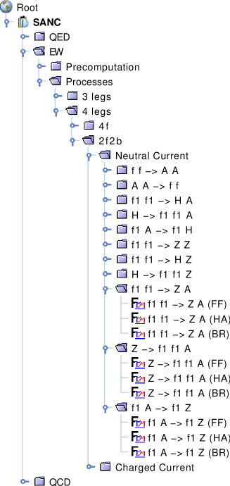
Figure 1: New processes in the $ffbb$ sector.

In the recent papers [7, 8] we presented an extension of the SANC Processes tree in the neutral current $ffbb$ sector, comprising the version V.1.10. In this paper we realize its further extension and include a calculation of the complete one-loop electroweak radiative corrections to the $Z$ boson production channels $f_{1}\bar{f}_{1}\to Z\gamma$ and $f_{1}\gamma\to f_{1}Z$, and to the $Z$ boson decay $Z\to f_{1}\bar{f}_{1}\gamma$. This class of processes was already mentioned in section 2.7 of Ref. [5]. For this reason, we do not change the number of SANC version, it is still V.1.10. The new processes are accessible from the $f_{1}f_{1}\to ZA$, $Z\to f_{1}f_{1}A$ and $f_{1}A\to f_{1}Z$ nodes, which are placed in the Neutral Current sector of node 2f2b on the electroweak part (EW) of the Processes tree, see Fig. 1. Each of these nodes contains standard modules of Scalar Form Factors (FF), Helicity Amplitudes (HA), and bremsstrahlung (BR).

The $Z\gamma$ production process is important for studies of the anomalous trilinear $Z\gamma\gamma$ and $ZZ\gamma$ gauge boson couplings at the Fermilab Tevatron[9, 10, 11], LHC[12, 13] and at the Linear Collider[14, 15] in both the $e^{+}e^{-}$ and $e\gamma$ modes. The Standard Model (SM) of electroweak interactions predicts no trilinear gauge coupling of the Z boson to the photon at the tree level. Any deviation of the couplings from the expected values would indicate the existence of new physics beyond the SM. At the LHC, it is expected to observe hundreds of thousands of events of vector boson pair production. To match the precision of the LHC experiments, the vector boson pair production processes have to be considered beyond leading order[16].

Leptonic final states of the $Z$ boson decays exhibit a very clear experimental signature and pave the way for precision tests of the SM beyond the leading order and possible detection of new physics. That is why it is necessary to fully control higher order EW corrections to the fermionic decays of the $Z$ boson.

These processes were considered in the literature earlier mostly in connection with their sensitivity to anomalous triple gauge couplings, see for example papers  [17, 18, 19, 20]. To our knowledge, the QED and EW corrections to the $Z$ boson production have been calculated previously only in papers  [21, 22, 23, 24].

All the processes under consideration can be treated as various cross channels of process $f_{1}\bar{f}_{1}Z\gamma\to 0$, and hence one-loop corrected scalar form factors, derived for this process, can be used for its cross channels also, after an appropriate permutation of their arguments ($s,t,u$). This is not the case for helicity amplitudes, however. They are different for all three channels and must be calculated separately.

The paper is organized as follows. In section 2 we demonstrate an analytic expression for the covariant amplitude at one-loop level in the annihilation channel. The helicity amplitudes for all three channels are given in section  3. In section 4 we present numerical results computed by FORTRAN codes generated with software s2n and comparison with other independent calculations. Finally, summary remarks are given in section 5.

2 Covariant Amplitude

Let us consider the process

$$\bar{f}_{1}(p_{1},\lambda_{1})+f_{1}(p_{2},\lambda_{2})+\gamma(p_{3},\lambda_{3})+Z(p_{4},\lambda_{4})\to 0,$$ (1)

where the 4-momenta $p_{i}$ $(i=1,2,3,4)$ of all external particles flow inwards. Here, $\lambda_{i}(i=1,2,3,4)$ are the helicities of corresponding particles. Schematically this process is given in Fig. 2, where the black blob represents the sum of all tree and one-loop self energy, vertex and box type Feynman diagrams contributing to this process. The contributions of the counter term diagrams coming from the OMS renormalization procedure is assumed, as well.

Figure 2: The $\bar{f_{1}}f_{1}\gamma Z\to 0$ process.

We found that next-to-leading order EW corrections to this process can be parameterized in terms of 28 scalar form factors (FF) and corresponding basic matrix elements, 14 vector and 14 axial ones. For the covariant amplitude (CA) we have:

$${\cal A}_{\bar{f_{1}}f_{1}Z\gamma}={\bar{v}}\left({p_{1}}\right)\left[{\rm Str}^{0}_{\mu\nu}\left(v_{f}{\cal F}^{0}_{v}+a_{f}\gamma_{5}{\cal F}^{0}_{a}\right)+\sum_{j=1}^{13}{\rm Str}^{j}_{\mu\nu}\left({\cal F}^{j}_{v}+\gamma_{5}{\cal F}^{j}_{a}\right)\right]u\left({p_{2}}\right)\varepsilon^{\gamma}_{\nu}(p_{3})\varepsilon^{Z}_{\mu}(p_{4}),$$ (2)

with

$${\rm Str}^{0}_{\mu\nu} = i\Biggl{[}\frac{1}{2}\Biggl{(}\frac{1}{U^{2}+m^{2}_{f}}+\frac{1}{T^{2}+m^{2}_{f}}\Biggr{)}\gamma_{\mu}/\!\!\!p_{3}\gamma_{\nu}+\frac{1}{U^{2}+m^{2}_{f}}\left(/\!\!\!p_{3}\delta_{\mu\nu}-\gamma_{\nu}(p_{3})_{\mu}\right)$$ (3)

$$-\Biggl{(}\frac{1}{U^{2}+m^{2}_{f}}(p_{1})_{\nu}-\frac{1}{T^{2}+m^{2}_{f}}(p_{2})_{\nu}\Biggr{)}\gamma_{\mu}\Biggr{]},$$

$${\rm Str}^{1}_{\mu\nu} = i\gamma_{\mu}/\!\!\!p_{3}\gamma_{\nu}\,,$$

$${\rm Str}^{2}_{\mu\nu} = /\!\!\!p_{3}\gamma_{\nu}(p_{1})_{\mu}\,,$$

$${\rm Str}^{3}_{\mu\nu} = /\!\!\!p_{3}\gamma_{\nu}(p_{2})_{\mu}\,,$$

$${\rm Str}^{4}_{\mu\nu} = \gamma_{\mu}\left[/\!\!\!p_{3}(p_{1})_{\nu}-\frac{1}{2}\left(U^{2}+m^{2}_{f}\right)\gamma_{\nu}\right],$$

$${\rm Str}^{5}_{\mu\nu} = \gamma_{\mu}\left[/\!\!\!p_{3}(p_{2})_{\nu}-\frac{1}{2}\left(T^{2}+m^{2}_{f}\right)\gamma_{\nu}\right],$$

$${\rm Str}^{6}_{\mu\nu} = i\left[/\!\!\!p_{3}(p_{1})_{\nu}-\frac{1}{2}\left(U^{2}+m^{2}_{f}\right)\gamma_{\nu}\right](p_{1})_{\mu},$$

$${\rm Str}^{7}_{\mu\nu} = i\left[/\!\!\!p_{3}(p_{2})_{\nu}-\frac{1}{2}\left(T^{2}+m^{2}_{f}\right)\gamma_{\nu}\right](p_{1})_{\mu},$$

$${\rm Str}^{8}_{\mu\nu} = i\left[/\!\!\!p_{3}(p_{1})_{\nu}-\frac{1}{2}\left(U^{2}+m^{2}_{f}\right)\gamma_{\nu}\right](p_{2})_{\mu},$$

$${\rm Str}^{9}_{\mu\nu} = i\left[/\!\!\!p_{3}(p_{2})_{\nu}-\frac{1}{2}\left(T^{2}+m^{2}_{f}\right)\gamma_{\nu}\right](p_{2})_{\mu},$$

$${\rm Str}^{10}_{\mu\nu} = i\left(/\!\!\!p_{3}\delta_{\mu\nu}-\gamma_{\nu}(p_{3})_{\mu}\right),$$

$${\rm Str}^{11}_{\mu\nu} = i\gamma_{\mu}\biggl{[}\left(T^{2}+m^{2}_{f}\right)(p_{1})_{\nu}-\left(U^{2}+m^{2}_{f}\right)(p_{2})_{\nu}\biggr{]},$$

$${\rm Str}_{12} = (p_{1})_{\mu}(p_{2})_{\nu}+(p_{2})_{\mu}(p_{2})_{\nu}+\frac{1}{2}\left(T^{2}+m^{2}_{f}\right)\delta_{\mu\nu},$$

$${\rm Str}^{13}_{\mu\nu} = \biggl{[}\left(T^{2}+m^{2}_{f}\right)(p_{1})_{\nu}-\left(U^{2}+m^{2}_{f}\right)(p_{2})_{\nu}\biggr{]}(p_{2})_{\mu},$$

where ${\bar{v}}\left({p_{1}}\right)$, $u\left({p_{2}}\right)$ and $m_{f}$ are the bispinors and the mass of the external fermions, respectively; $\varepsilon^{\gamma}_{\nu}(p_{3})$ denotes the photon polarization vector and $\varepsilon^{Z}_{\mu}(p_{4})$ is the $Z$ boson polarization vector; the vector and axial gauge-boson-to-fermion couplings are denoted by $v_{f}$ and $a_{f}$, respectively; ${\cal F}^{j}_{v,a}$ are the scalar FF of the vector and axial vector currents, respectively; ${\cal F}^{0}_{v,a}$ and ${\rm Str}^{0}_{\mu\nu}$ correspond to the lowest-order matrix elements. The usual Mandelstam invariants in Pauli metric ($p^{2}=-m^{2}$) are defined as follows:

$$(p_{1}+p_{2})^{2}=Q^{2}=-s,$$

$$(p_{2}+p_{3})^{2}=T^{2}=-t,$$

$$(p_{2}+p_{4})^{2}=U^{2}=-u.$$ (4)

In Eq.(2) we keep the fermion mass in order to maintain photon transversality. Moreover in mass-containing denominators of ${\rm Str}^{0}_{\mu\nu}$, the mass cannot be neglected because these denominators correspond to the propagators of fermions which emit external photons and thus would lead to mass singularities.

The basic matrix elements, ${\rm Str}^{j}_{\mu\nu}$, are chosen to be explicitly transverse to the photonic 4-momentum. That is, for all of them the following relations hold:

$${\rm Str}^{j}_{\mu\nu}(p_{3})_{\nu}=0.$$ (5)

We have checked that the FF ${\cal F}^{j}_{v,a}$ are free of gauge parameters and of ultraviolet singularities (all calculations are done in the $R_{\xi}$ gauge). The analytical expressions of the FF are too cumbersome to be presented in this paper. They can be reproduced on-line with help of the SANC system. The CA for the processes we are interested in can be obtained from Eq.(2) exploiting crossing symmetry. This subject is covered in the next section.

3 Helicity Amplitudes

In this section we collect the analytical expressions of the helicity amplitudes (HA) for all three channels. Let us briefly recall the SANC strategy of observable (cross section, differential distributions) calculations. In a first step, SANC constructs the CA of the process, free of gauge parameters and of ultraviolet singularities, taking into account all lowest order and one-loop Feynman diagrams that contribute to the process. In the next step, HA are calculated analytically and converted into numerical code. Further, the cross section or the decay width of the process is formed as the incoherent sum of squares of all possible HA:

$$d\sigma(d\Gamma)\sim\sum_{\lambda_{1}\lambda_{2}...\lambda_{n}}|{\cal H}_{\lambda_{1}\lambda_{2}...\lambda_{n}}|^{2}\,d\Phi^{n}$$ (6)

where squaring and summing is performed numerically. And finally, the Monte Carlo integrations over phase-space $d\Phi^{n}$ are performed using Vegas routine [25].

3.1 Annihilation channel $\bar{f}_{1}f_{1}\to Z\gamma$

To obtain the CA for the process

$$\bar{f}_{1}(p_{1},\lambda_{1})+f_{1}(p_{2},\lambda_{2})\to\gamma(p_{3},\lambda_{3})+Z(p_{4},\lambda_{4}),$$ (7)

where $\lambda_{i}(i=1,2,3,4)$ are the helicities of the external particles, we use the following substitutions of 4-momenta in Eq.(2):

$$\begin{array}[]{llll}&p_{1}&\to&~{}~{}p_{1},\\ &p_{2}&\to&~{}~{}p_{2},\\ &p_{3}&\to&-p_{3},\\ &p_{4}&\to&-p_{4}.\\ \end{array}$$

Figure 3: Schematic representation of one-loop Feynman diagrams for the annihilation channel.

The set of non-vanishing HA for this process, which we denote as ${\cal H}_{\lambda_{1}\lambda_{2}\lambda_{3}\lambda_{4}}$, read:

$${\cal H}_{\mp\mp\mp\mp} = \frac{m_{f}}{\sqrt{s}}\left[2-\frac{1}{2}\frac{sZ_{4}(M_{Z})}{Z_{1}(m_{f})Z_{2}(m_{f})}\sin^{2}\vartheta_{\gamma}\right]v_{f}{\cal F}_{v0}$$

$$+\frac{Z_{4}(M_{\scriptscriptstyle{Z}})}{4\sqrt{s}}c_{-}\Biggl{[}c_{+}\Bigl{(}{\cal F}_{2}^{\pm}-{\cal F}_{3}^{\pm}-{\cal F}_{4}^{\pm}\Bigr{)}-c_{-}{\cal F}_{5}^{\pm}+{\cal F}_{12}^{\pm}-\frac{s}{2}c_{+}{\cal F}_{13}^{\pm}\Biggr{]},$$

$${\cal H}_{\mp\mp\mp 0} = \mp\frac{Z_{4}(M_{\scriptscriptstyle{Z}})}{4\sqrt{2}M_{\scriptscriptstyle{Z}}}\sin\vartheta_{\gamma}\Biggl{[}\frac{4M_{\scriptscriptstyle{Z}}^{2}m_{f}}{Z_{1}(m_{f})Z_{2}(m_{f})}\cos\vartheta_{\gamma}v_{f}{\cal F}_{v0}$$

$$+k_{2}{\cal F}_{2}^{\pm}+k_{1}{\cal F}_{3}^{\pm}-k_{2}{\cal F}_{4}^{\pm}+k_{+}c_{-}{\cal F}_{5}^{\pm}-s{\cal F}_{12}^{\pm}+\frac{s}{2}k_{1}{\cal F}_{13}^{\pm}\Biggr{]},$$

$${\cal H}_{\mp\mp\mp\pm} = \frac{\sqrt{s}}{4}Z_{4}(M_{\scriptscriptstyle{Z}})\sin^{2}\vartheta_{\gamma}\Biggl{[}\frac{2m_{f}}{Z_{1}(m_{f})Z_{2}(m_{f})}v_{f}{\cal F}_{v0}-{\cal F}_{2}^{\pm}+{\cal F}_{3}^{\pm}+{\cal F}_{4}^{\pm}-{\cal F}_{5}^{\pm}+\frac{s}{2}{\cal F}_{13}^{\pm}\Biggr{]},$$

$${\cal H}_{\mp\mp\pm\mp} = \frac{\sqrt{s}}{8}Z_{4}(M_{\scriptscriptstyle{Z}})\sin^{2}\vartheta_{\gamma}\Biggl{[}\frac{4m_{f}}{Z_{1}(m_{f})Z_{2}(m_{f})}v_{f}{\cal F}_{v0}+s{\cal F}_{13}^{\pm}\Biggr{]},$$

$${\cal H}_{\mp\mp\pm 0} = \pm\frac{Z_{4}(M_{\scriptscriptstyle{Z}})}{\sqrt{2}M_{\scriptscriptstyle{Z}}}\sin\vartheta_{\gamma}\Biggl{[}\frac{m_{f}}{Z_{1}(m_{f})Z_{2}(m_{f})}\left(M_{\scriptscriptstyle{Z}}^{2}\cos\vartheta_{\gamma}v_{f}{\cal F}_{v0}\pm Z_{4}(M_{\scriptscriptstyle{Z}})a_{f}{\cal F}_{a0}\right)$$

$$-\frac{s}{4}\Bigl{(}2{\cal F}_{4}^{\pm}+{\cal F}_{12}^{\pm}-\frac{1}{2}k_{1}{\cal F}_{13}^{\pm}\Bigr{)}\Biggr{]},$$

$${\cal H}_{\mp\mp\pm\pm} = \frac{m_{f}}{2\sqrt{s}}\Biggl{[}\left(4-\left(2Z_{4}(M_{\scriptscriptstyle{Z}})+s\sin^{2}\vartheta_{\gamma}\right)\frac{Z_{4}(M_{\scriptscriptstyle{Z}})}{Z_{1}(m_{f})Z_{2}(m_{f})}\right)v_{f}{\cal F}_{v0}$$

$$\pm 2\frac{Z^{2}_{4}(M_{\scriptscriptstyle{Z}})}{Z_{1}(m_{f})Z_{2}(m_{f})}\cos\vartheta_{\gamma}a_{f}{\cal F}_{a0}\Biggr{]}-\frac{\sqrt{s}}{2}Z_{4}(M_{\scriptscriptstyle{Z}})\left(c_{+}{\cal F}_{4}^{\pm}-\frac{1}{2}c_{-}{\cal F}_{12}^{\pm}+\frac{s}{4}\sin^{2}\vartheta_{\gamma}{\cal F}_{13}^{\pm}\right),$$

$${\cal H}_{\pm\mp\pm\pm} = \mp\frac{1}{8}\sin\vartheta_{\gamma}\Biggl{[}\frac{4M_{\scriptscriptstyle{Z}}^{2}}{Z_{1}(m_{f})}{\cal F}_{0}^{\pm}-Z_{4}(M_{\scriptscriptstyle{Z}})\left[sc_{+}\left({\cal F}_{6}^{\pm}-{\cal F}_{8}^{\pm}\right)+4{\cal F}_{10}^{\pm}+2sc_{-}{\cal F}_{11}^{\pm}\right]\Biggr{]},$$

$${\cal H}_{\pm\mp\mp\mp} = \pm\frac{1}{8}\sin\vartheta_{\gamma}\Biggl{[}\frac{4M_{\scriptscriptstyle{Z}}^{2}}{Z_{2}(m_{f})}{\cal F}_{0}^{\pm}-Z_{4}(M_{\scriptscriptstyle{Z}})\left[8{\cal F}_{1}^{\pm}+sc_{-}\left({\cal F}_{7}^{\pm}-{\cal F}_{9}^{\pm}\right)-4{\cal F}_{10}^{\pm}+2sc_{+}{\cal F}_{11}^{\pm}\right]\Biggr{]},$$

$${\cal H}_{\pm\mp\pm 0} = \frac{1}{8\sqrt{2}}\frac{\sqrt{s}}{M_{\scriptscriptstyle{Z}}}c_{+}\Biggl{[}\frac{8M_{\scriptscriptstyle{Z}}^{2}}{Z_{1}(m_{f})}{\cal F}_{0}^{\pm}+Z_{4}(M_{\scriptscriptstyle{Z}})\left(k_{2}{\cal F}_{6}^{\pm}+k_{1}{\cal F}_{8}^{\pm}-4{\cal F}_{10}^{\pm}-2k_{+}c_{-}{\cal F}_{11}^{\pm}\right)\Biggr{]},$$

$${\cal H}_{\mp\pm\pm 0} = -\frac{1}{8\sqrt{2}}\frac{\sqrt{s}}{M_{\scriptscriptstyle{Z}}}c_{-}\Biggl{[}\frac{8M_{\scriptscriptstyle{Z}}^{2}}{Z_{2}(m_{f})}{\cal F}_{0}^{\pm}-Z_{4}(M_{\scriptscriptstyle{Z}})\left(8{\cal F}_{1}^{\pm}+k_{2}{\cal F}_{7}^{\pm}+k_{1}{\cal F}_{9}^{\pm}-4{\cal F}_{10}^{\pm}+2k_{+}c_{+}{\cal F}_{11}^{\pm}\right)\Biggr{]},$$

$${\cal H}_{\pm\mp\pm\mp} = \mp\frac{s}{8}Z_{4}(M_{\scriptscriptstyle{Z}})\sin\vartheta_{\gamma}c_{+}\Biggl{[}\frac{2}{Z_{1}(m_{f})Z_{2}(m_{f})}{\cal F}_{0}^{\pm}+{\cal F}_{6}^{\pm}-{\cal F}_{8}^{\pm}-2{\cal F}_{11}^{\pm}\Biggr{]},$$

$${\cal H}_{\pm\mp\mp\pm} = \pm\frac{s}{8}Z_{4}(M_{\scriptscriptstyle{Z}})\sin\vartheta_{\gamma}c_{-}\Biggl{[}\frac{2}{Z_{1}(m_{f})Z_{2}(m_{f})}{\cal F}_{0}^{\pm}+{\cal F}_{7}^{\pm}-{\cal F}_{9}^{\pm}-2{\cal F}_{11}^{\pm}\Biggr{]},$$ (8)

with the following shorthand notation

$${\cal F}^{\pm}_{0} = v_{f}{\cal F}_{v0}(s,t,u)\pm a_{f}{\cal F}_{a0}(s,t,u),$$

$${\cal F}^{\pm}_{j} = {\cal F}_{vj}(s,t,u)\pm{\cal F}_{aj}(s,t,u),\qquad j=1,...13,$$

$$k_{1,2} = sc_{\pm}-M_{\scriptscriptstyle{Z}}^{2}c_{\mp}\,,\;\;\;c_{\pm}=1\pm\cos\vartheta_{\gamma}\,,$$

$$Z_{1}(m_{f}) = \frac{1}{2}Z_{4}(M_{\scriptscriptstyle{Z}})\left(1+\beta\cos{\vartheta_{\gamma}}\right),\quad\beta\equiv\beta_{f}=\sqrt{1-4m^{2}_{f}/s},$$

$$Z_{2}(m_{f}) = \frac{1}{2}Z_{4}(M_{\scriptscriptstyle{Z}})\left(1-\beta\cos{\vartheta_{\gamma}}\right),$$

$$Z_{4}(M_{\scriptscriptstyle{Z}}) = s-M_{\scriptscriptstyle{Z}}^{2}.$$ (9)

Here $\vartheta_{\gamma}$ is the center of mass system angle of the produced photon (angle between momenta $\vec{p}_{2}$ and $\vec{p}_{3}$), $t$ and $u$ are the Mandelstam variables:

$$t=m_{f}^{2}-Z_{2}(m_{f}),\qquad u=m_{f}^{2}-Z_{1}(m_{f}).$$ (10)

3.2 Decay channel $Z\to f_{1}\bar{f}_{1}\gamma$

The CA of $Z$ boson decay into fermion anti-fermion pairs and one real photon,

$$Z(p_{2},\lambda_{2})\to\gamma(p_{1},\lambda_{1})+f_{1}(p_{3},\lambda_{3})+\bar{f}_{1}(p_{4},\lambda_{4}),$$ (11)

is obtained by interchanging of 4-momenta in Eq.(2) as follows:

$$\begin{array}[]{llll}&p_{1}&\to&-p_{3},\\ &p_{2}&\to&-p_{4},\\ &p_{3}&\to&-p_{1},\\ &p_{4}&\to&~{}~{}p_{2}.\end{array}$$

Figure 4: Schematic representation of one-loop Feynman diagrams for the decay channel.

For the non-vanishing HA, ${\cal H}_{\lambda_{2}\lambda_{1}\lambda_{3}\lambda_{4}}$, we have

$${\cal H}_{\pm\pm\pm\pm} = -\frac{\sqrt{s}}{8}Z_{2}(M_{\scriptscriptstyle{Z}})\sin^{2}\vartheta_{f}\Biggl{[}\frac{4m_{f}}{Z_{3}(m_{f})Z_{4}(m_{f})}v_{f}{\cal F}_{v0}+s{\cal F}_{13}^{\pm}\Biggr{]},$$

$${\cal H}_{\mp\mp\mp\pm} = \mp\frac{s}{8}Z_{2}(M_{\scriptscriptstyle{Z}})\sin\vartheta_{f}c_{+}\Biggl{[}\frac{2}{Z_{3}(m_{f})Z_{4}(m_{f})}{\cal F}^{\pm}_{0}+{\cal F}_{7}^{\pm}-{\cal F}_{9}^{\pm}-2{\cal F}_{11}^{\pm}\Biggr{]},$$

$${\cal H}_{\pm\pm\mp\pm} = \pm\frac{s}{8}Z_{2}(M_{\scriptscriptstyle{Z}})\sin\vartheta_{f}c_{-}\Biggl{[}\frac{2}{Z_{3}(m_{f})Z_{4}(m_{f})}{\cal F}^{\pm}_{0}+{\cal F}_{6}^{\pm}-{\cal F}_{8}^{\pm}-2{\cal F}_{11}^{\pm}\Biggr{]},$$

$${\cal H}_{\mp\pm\mp\pm} = \mp\frac{1}{8}\sin\vartheta_{f}\Biggl{[}4\frac{M_{\scriptscriptstyle{Z}}^{2}}{Z_{3}(m_{f})}{\cal F}^{\pm}_{0}-Z_{2}(M_{\scriptscriptstyle{Z}})\Biggl{(}sc_{-}\left({\cal F}_{6}^{\pm}-{\cal F}_{8}^{\pm}\right)+4{\cal F}_{10}^{\pm}+2sc_{+}{\cal F}_{11}^{\pm}\Biggr{)}\Biggr{]},$$

$${\cal H}_{\pm\mp\mp\pm} = \pm\frac{1}{8}\sin\vartheta_{f}\Biggl{[}4\frac{M_{\scriptscriptstyle{Z}}^{2}}{Z_{4}(m_{f})}{\cal F}^{\pm}_{0}-Z_{2}(M_{\scriptscriptstyle{Z}})\Biggl{(}8{\cal F}_{1}^{\pm}+sc_{+}\left({\cal F}_{7}^{\pm}-{\cal F}_{9}^{\pm}\right)-4{\cal F}_{10}^{\pm}+2sc_{-}{\cal F}_{11}^{\pm}\Biggr{)}\Biggr{]},$$

$${\cal H}_{\mp\mp\pm\pm} = -\frac{1}{8}\sqrt{s}Z_{2}(M_{\scriptscriptstyle{Z}})\sin^{2}\vartheta_{f}\Biggl{[}\frac{4m_{f}}{Z_{3}(m_{f})Z_{4}(m_{f})}v_{f}{\cal F}_{v0}-2\left({\cal F}_{2}^{\pm}-{\cal F}_{3}^{\pm}-{\cal F}_{4}^{\pm}+{\cal F}_{5}^{\pm}\right)+s{\cal F}_{13}^{\pm}\Biggr{]},$$

$${\cal H}_{\pm\mp\pm\pm} = -\frac{1}{4}\sqrt{s}\Biggl{[}8\frac{m_{f}}{s}\frac{M_{\scriptscriptstyle{Z}}^{2}}{Z_{2}(M_{\scriptscriptstyle{Z}})}v_{f}{\cal F}_{v0}$$

$$\hskip 28.45274pt-Z_{2}(M_{\scriptscriptstyle{Z}})\Biggl{(}\sin^{2}\vartheta_{f}\Bigl{(}{\cal F}_{2}^{\pm}-{\cal F}_{3}^{\pm}-{\cal F}_{4}^{\pm}\Bigr{)}-c_{+}^{2}{\cal F}_{5}^{\pm}+c_{+}{\cal F}_{12}^{\pm}+\frac{s}{2}\sin^{2}\vartheta_{f}{\cal F}_{13}^{\pm}\Biggr{)}\Biggr{]},$$

$${\cal H}_{\mp\pm\pm\pm} = -\frac{1}{2}\sqrt{s}\Biggl{[}4\frac{m_{f}}{s}\frac{M_{\scriptscriptstyle{Z}}^{2}}{Z_{2}(M_{\scriptscriptstyle{Z}})}v_{f}{\cal F}_{v0}-2\frac{m_{f}}{s}\frac{Z^{2}_{2}(M_{\scriptscriptstyle{Z}})}{Z_{3}(m_{f})Z_{4}(m_{f})}\left(v_{f}{\cal F}_{v0}\pm\cos\vartheta_{f}a_{f}{\cal F}_{a0}\right)$$

$$\hskip 28.45274pt+Z_{2}(M_{\scriptscriptstyle{Z}})\Biggl{(}c_{-}{\cal F}_{4}^{\pm}-\frac{1}{2}c_{+}{\cal F}_{12}^{\pm}+\frac{s}{4}\sin^{2}\vartheta_{f}{\cal F}_{13}^{\pm}\Biggr{)}\Biggr{]},$$

$${\cal H}_{0\pm\pm\pm} = \frac{i}{8\sqrt{2}}\frac{sZ_{2}(M_{\scriptscriptstyle{Z}})}{M_{\scriptscriptstyle{Z}}}\sin\vartheta_{f}\Biggl{[}\frac{8m_{f}}{sZ_{3}(m_{f})Z_{4}(m_{f})}\left(M_{\scriptscriptstyle{Z}}^{2}\cos\vartheta_{f}v_{f}{\cal F}_{v0}\pm{Z_{2}(M_{\scriptscriptstyle{Z}})}a_{f}{\cal F}_{a0}\right)$$

$$\hskip 28.45274pt+4{\cal F}_{4}^{\pm}+2{\cal F}_{12}^{\pm}-k_{2}{\cal F}_{13}^{\pm}\Biggl{]},$$

$${\cal H}_{0\mp\pm\pm} = \frac{i}{4\sqrt{2}}\frac{Z_{2}(M_{\scriptscriptstyle{Z}})}{M_{\scriptscriptstyle{Z}}}\sin\vartheta_{f}\Biggl{[}\frac{4sm_{f}}{Z_{3}(m_{f})Z_{4}(m_{f})}\cos\vartheta_{f}v_{f}{\cal F}_{v0}$$

$$\hskip 28.45274pt-k_{1}{\cal F}_{2}^{\pm}-k_{2}{\cal F}_{3}^{\pm}+k_{1}{\cal F}_{4}^{\pm}-k_{+}c_{+}{\cal F}_{5}^{\pm}+s{\cal F}_{12}^{\pm}-\frac{s}{2}k_{2}{\cal F}_{13}^{\pm}\Biggl{]},$$

$${\cal H}_{0\mp\mp\pm} = \mp\frac{i}{\sqrt{2}}\frac{\sqrt{s}}{M_{\scriptscriptstyle{Z}}}\Biggl{[}2\frac{M_{\scriptscriptstyle{Z}}^{2}}{Z_{2}(M_{\scriptscriptstyle{Z}})}{\cal F}^{\pm}_{0}-\frac{1}{8}Z_{2}(M_{\scriptscriptstyle{Z}})c_{+}\Biggl{(}8{\cal F}_{1}^{\pm}+k_{1}{\cal F}_{7}^{\pm}+k_{2}{\cal F}_{9}^{\pm}-4{\cal F}_{10}^{\pm}+2k_{+}c_{-}{\cal F}_{11}^{\pm}\Biggr{)}\Biggr{]},$$

$${\cal H}_{0\pm\mp\pm} = \mp\frac{i}{8\sqrt{2}}\frac{\sqrt{s}}{M_{\scriptscriptstyle{Z}}}\Biggl{[}2\frac{M_{\scriptscriptstyle{Z}}^{2}}{Z_{2}(M_{\scriptscriptstyle{Z}})}{\cal F}^{\pm}_{0}+\frac{1}{8}Z_{2}(M_{\scriptscriptstyle{Z}})c_{-}\Biggl{(}k_{1}{\cal F}_{6}^{\pm}+k_{2}{\cal F}_{8}^{\pm}-4{\cal F}_{10}^{\pm}-2k_{+}c_{+}{\cal F}_{11}^{\pm}\Biggl{)}\Biggr{]},$$ (12)

where ${\cal F}^{\pm}_{j}$ and the coefficients $k_{1,2}$ are defined by Eqs. (9) and (10) with $c_{\pm}=1\pm\cos\vartheta_{f}$, and

$$Z_{3}(m_{f})=\frac{1}{2}Z_{2}(M_{\scriptscriptstyle{Z}})\left(1+\beta\cos{\vartheta_{f}}\right),\qquad\beta=\sqrt{1-4m_{f}^{2}/s},$$

$$Z_{4}(m_{f})=\frac{1}{2}Z_{2}(M_{\scriptscriptstyle{Z}})\left(1-\beta\cos{\vartheta_{f}}\right),$$

$$s=M^{2}_{f\bar{f}},\quad t=m_{f}^{2}+Z_{4}(m_{f}),\quad u=m_{f}^{2}+Z_{3}(m_{f}).$$ (13)

Here $Z_{2}(M_{\scriptscriptstyle{Z}})=M_{\scriptscriptstyle{Z}}^{2}-s$ and $\vartheta_{f}$ is the angle between the vector $\vec{p}_{3}$ and the direction defined by the photon momentum $\vec{p}_{1}$ in the rest frame of compound $(\vec{p}_{3},\vec{p}_{4})$. The photon momentum, $\vec{p}_{1}$, is chosen to be direction of the $z$-axes in the $(\vec{p}_{3},\vec{p}_{4})$ rest frame.

3.3 $Z$ production channel $e\gamma\to eZ$

And finally, in order to obtain the CA for the $Z$ boson production channel

$$\gamma(p_{1},\lambda_{1})+e^{\pm}(p_{2},\lambda_{2})\to e^{\pm}(p_{3},\lambda_{3})+Z(p_{4},\lambda_{4})$$ (14)

from Eq.(2), the 4-momenta permutations must be chosen as follows:

$$\begin{array}[]{llll}&p_{1}&\to&-p_{3},\\ &p_{2}&\to&-p_{4},\\ &p_{3}&\to&-p_{1},\\ &p_{4}&\to&~{}~{}p_{2}.\end{array}$$

Figure 5: Schematic representation of one-loop Feynman diagrams for the $Z$ boson production channel.

The HA, ${\cal H}_{\lambda_{1}\lambda_{2}\lambda_{3}\lambda_{4}}$, for this channel read

$${\cal H}_{\pm\mp\mp\pm} = \frac{k_{3}}{\sqrt{2s}}\Biggl{[}2\left(\frac{1}{k_{-}}-\frac{1}{Z_{3}(m_{e})}\right)M_{\scriptscriptstyle{Z}}^{2}{\cal F}_{0}^{\pm}+sc_{-}\left(\frac{k_{-}}{4}c_{+}{\cal F}_{8}^{\pm}-{\cal F}_{10}^{\pm}+k_{-}{\cal F}_{11}^{\pm}\right)\Biggr{]},$$

$${\cal H}_{\pm\mp\mp 0} = \pm\frac{k_{4}}{M_{\scriptscriptstyle{Z}}}\Biggl{[}\frac{2M_{\scriptscriptstyle{Z}}^{2}}{k_{-}}{\cal F}_{0}^{\pm}+\frac{1}{2}c_{+}\left(\frac{k_{-}^{2}}{2}{\cal F}_{6}^{\pm}-\frac{k_{-}}{4}k_{1}{\cal F}_{8}^{\pm}+k_{+}{\cal F}_{10}^{\pm}-sk_{-}{\cal F}_{11}^{\pm}\right)\Biggr{]},$$

$${\cal H}_{\pm\mp\pm 0} = \frac{k_{3}}{M_{\scriptscriptstyle{Z}}\sqrt{s}}\Biggl{[}\frac{2m_{e}}{Z_{3}(m_{e})}\Biggl{(}M_{\scriptscriptstyle{Z}}^{2}\left(\frac{s}{k_{-}}+1\right)v_{e}{\cal F}_{v_{0}}\pm\frac{s^{2}}{k_{-}}a_{e}{\cal F}_{a_{0}}\Biggr{)}$$

$$+\frac{s}{4}c_{-}\left(2k_{-}{\cal F}_{4}^{\pm}+k_{+}{\cal F}_{12}^{\pm}-\frac{k_{-}}{2}k_{1}{\cal F}_{13}^{\pm}\right)\Biggr{]},$$

$$\ {\cal H}_{\pm\mp\pm\pm} = \mp\frac{k_{4}}{\sqrt{2}}\Biggl{[}\frac{2sm_{e}}{Z_{3}(m_{e})k_{-}}{\cal F}_{v_{0}}^{\pm}+\frac{s}{2}c_{-}\left({\cal F}_{12}^{\pm}-\frac{k_{-}}{2}c_{+}{\cal F}_{13}^{\pm}\right)\Biggr{]},$$

$${\cal H}_{\pm\mp\pm\mp} = \mp\frac{k_{4}}{\sqrt{2}}c_{+}\Biggl{[}k_{-}{\cal F}_{4}^{\pm}+\frac{s}{2}\left({\cal F}_{12}^{\pm}+\frac{k_{-}}{2}c_{-}{\cal F}_{13}^{\pm}\right)\Biggr{]},$$

$${\cal H}_{\mp\mp\pm 0} = -\frac{\sqrt{s}k_{3}}{M_{\scriptscriptstyle{Z}}}\Biggl{[}\frac{2M_{\scriptscriptstyle{Z}}^{2}m_{e}}{sZ_{3}(m_{e})}v_{e}{\cal F}_{v_{0}}$$

$$-k_{-}{\cal F}_{2}^{\pm}+\frac{1}{2}k_{1}{\cal F}_{3}^{\pm}+k_{-}{\cal F}_{4}^{\pm}-s{\cal F}_{5}^{\pm}+\frac{1}{4}c_{-}\left(k_{+}{\cal F}_{12}^{\pm}-\frac{k_{-}}{2}k_{1}{\cal F}_{13}^{\pm}\right)\Biggr{]},$$

$${\cal H}_{\mp\mp\mp\mp} = \left(\frac{s}{2}\right)^{\frac{3}{2}}k_{3}c_{-}{\cal F}_{9}^{\pm},$$

$${\cal H}_{\mp\mp\mp 0} = \pm\frac{sk_{4}}{M_{\scriptscriptstyle{Z}}}\Biggl{[}2{\cal F}_{1}^{\pm}-\frac{k_{-}}{2}{\cal F}_{7}^{\pm}+\frac{1}{4}k_{1}{\cal F}_{9}^{\pm}-{\cal F}_{10}^{\pm}+\frac{k_{-}}{2}c_{+}{\cal F}_{11}^{\pm}\Biggr{]},$$

$${\cal H}_{\mp\mp\mp\pm} = -\frac{k_{3}}{\sqrt{2s}}\Biggl{[}\frac{2k_{-}}{Z_{3}(m_{e})}{\cal F}_{0}^{\pm}-s\left(4{\cal F}_{1}^{\pm}-\frac{s}{2}c_{-}{\cal F}_{9}^{\pm}-2{\cal F}_{10}^{\pm}-k_{-}c_{-}{\cal F}_{11}^{\pm}\right)\Biggr{]},$$

$${\cal H}_{\mp\mp\pm\mp} = \mp\frac{sk_{4}}{\sqrt{2}}\Biggl{[}c_{+}{\cal F}_{3}^{\pm}-2{\cal F}_{5}^{\pm}+\frac{1}{2}c_{-}\left({\cal F}_{12}^{\pm}-\frac{k_{-}}{2}c_{+}{\cal F}_{13}^{\pm}\right)\Biggr{]},$$

$${\cal H}_{\mp\mp\pm\pm} = \pm\frac{sk_{4}}{\sqrt{2}}c_{+}\Biggl{[}{\cal F}_{3}^{\pm}-\frac{1}{2}{\cal F}_{12}^{\pm}-\frac{k_{-}}{4}c_{-}{\cal F}_{13}^{\pm}\Biggr{]},$$

$${\cal H}_{\pm\mp\mp\mp} = -\sqrt{\frac{s}{2}}k_{3}\Biggl{[}\frac{2}{k_{-}}{\cal F}_{0}^{\pm}+c_{+}\left(\frac{k_{-}}{4}c_{-}{\cal F}_{8}^{\pm}+{\cal F}_{10}^{\pm}\right)\Biggr{]}.$$ (15)

Here the coefficients $k_{3,4,\pm}$ are defined by

$$k_{3}=N_{-}\cos\frac{\vartheta_{e}}{2},\qquad k_{4}=N_{-}\sin\frac{\vartheta_{e}}{2},\qquad k_{\pm}=s\pm M_{\scriptscriptstyle{Z}}^{2},$$ (16)

with

$$N_{-}=\sqrt{\frac{s-M_{\scriptscriptstyle{Z}}^{2}}{2}}\,,$$ (17)

$Z_{2}(m_{e})$ and $Z_{3}(m_{e})$ are the denominators of fermionic propagators:

$$Z_{2}(m_{e})=s-m_{e}^{2}\,,$$

$$Z_{3}(m_{e})=\frac{Z_{2}(m_{e})}{2s}\left[s+m_{e}^{2}-M_{\scriptscriptstyle{Z}}^{2}+\sqrt{\lambda(s,m_{e}^{2},M_{\scriptscriptstyle{Z}}^{2})}\cos\vartheta_{e}\right],$$ (18)

and $\vartheta_{e}$ denotes the $e^{\pm}$ scattering angle. The Mandelstam variables transform as follows:

$$s\rightarrow-\frac{1}{2}\left[\left(s-\frac{M_{\scriptscriptstyle{Z}}^{2}m_{e}^{2}}{s}-M_{\scriptscriptstyle{Z}}^{2}-2m_{e}^{2}+\frac{m_{e}^{4}}{s}\right)-\frac{s-m_{e}^{2}}{s}\sqrt{\lambda(s,m_{e}^{2},M_{\scriptscriptstyle{Z}}^{2})}\cos\vartheta_{e}\right],$$

$$u\rightarrow-\frac{1}{2}\left[\left(s+\frac{M_{\scriptscriptstyle{Z}}^{2}m_{e}^{2}}{s}-M_{\scriptscriptstyle{Z}}^{2}-2m_{e}^{2}-\frac{m_{e}^{4}}{s}\right)+\frac{s-m_{e}^{2}}{s}\sqrt{\lambda(s,m_{e}^{2},M_{\scriptscriptstyle{Z}}^{2})}\cos\vartheta_{e}\right],$$

$$t\rightarrow s.$$

4 Numerical results and comparison

In this section we present the SANC predictions for various observables of all three processes under consideration. The tree level and single real photon emission contributions are compared with CompHEP, while one-loop electroweak and QED corrections for the production channel $e\gamma\to eZ$ are checked against the Grace-loop package [4] and Ref. [24]. Note that all numerical results of this section are produced with the Standard SANC INPUT (section 6.2.3 of Ref. [8]) if not stated otherwise.

4.1 Annihilation channel $\bar{f}_{1}f_{1}\to Z\gamma$

For this process we show in Table 1 a comparison between SANC and CompHEP results for the Born level cross sections and the cross sections of hard photon radiation.

	$\sigma$, pb
$\sqrt{s}$, GeV	100	200	500	1000	2000
Born (SANC )	2482.0(1)	86.230(1)	11.652(1)	2.9845(1)	0.77816(1)
Born (CompHEP)	2482.0(1)	86.230(1)	11.651(1)	2.9846(1)	0.77817(1)
Hard (SANC )	586.7(7)	43.26(8)	7.69(2)	2.341(6)	0.717(2)
Hard (CompHEP)	586.7(3)	42.48(5)	7.47(1)	unstable	unstable

Table 1: Comparison of the Born and Hard cross sections of the $e^{+}e^{-}\to Z\gamma(\gamma)$ process (CompHEP input, $E_{\gamma}\geq 1$ GeV). The uncertainty of the last significant digit is given in brackets.

	$\sigma$, pb
$\sqrt{s}$, GeV	100	200	500	1000	2000
Born (SANC )	1349.5(1)	49.086(1)	6.9785(1)	1.8469(1)	0.49555(1)
Born (CompHEP)	1349.4(1)	49.086(1)	6.9786(1)	1.8469(1)	0.49555(1)
Hard (SANC )	173.82(3)	14.138(3)	2.7978(9)	0.9228(4)	0.3024(2)
Hard (CompHEP)	173.82(3)	14.083(21)	2.7627(21)	0.9045(11)	0.2936(4)

Table 2: The same as Table 1 but for the process $\mu^{+}\mu^{-}\to Z\gamma(\gamma)$.

As can be seen from Table 1, we found very good agreement for the Born cross section. For the hard contribution we have perfect agreement at $\sqrt{s}=$100 GeV, then a difference rapidly rising with energy, and eventually unstable CompHEP predictions for $\sqrt{s}$ at and above 1 TeV. As seen from Table 2 for the process $\mu^{+}\mu^{-}\to Z\gamma(\gamma)$, the hard contributions stay closer (though statistically incompatible) within a wider range of $\sqrt{s}$ pointing to the origin of the difference due to collinear singularities of the integrand. The stability against variation of $\bar{\omega}$ discussed below gives us a great level of confidence in the SANC results.

In Tables 3–5 we present the results of our calculations for the annihilation channels $e^{+}e^{-}\to Z\gamma(\gamma)$, $\bar{u}u\to Z\gamma(\gamma)$ and $\bar{d}d\to Z\gamma(\gamma)$, respectively, carried out with 10M statistics for the hard cross section for five energies and at each energy for two values of $\bar{\omega}$: $\bar{\omega}=10^{-5}\sqrt{s}/2$ (subscript 1) and $10^{-6}\sqrt{s}/2$ (subscript 2); for $\sigma$’s in pb and for $\delta=\sigma^{\rm 1-loop}/\sigma^{\rm Born}-1$ in %.

$\sqrt{s}$, GeV	200	500	1000	2000	5000
$\sigma^{\rm Born}$, pb	27.8548(1)	3.37334(1)	0.816485(2)	0.202534(1)	0.0323355(1)
$\sigma^{\rm 1-loop}_{1}$, pb	43.36(4)	5.216(9)	1.239(4)	0.299(1)	0.0436(3)
$\sigma^{\rm 1-loop}_{2}$, pb	43.38(5)	5.211(10)	1.235(4)	0.298(2)	—
$\delta_{1}$, %	55.7(2)	54.6(3)	51.9(4)	47.4(6)	34.9(8)
$\delta_{2}$, %	55.7(2)	54.5(3)	51.3(5)	46.9(8)	—

Table 3: Comparison of the Born and one-loop cross sections of the annihilation channel $e^{+}e^{-}\to Z\gamma(\gamma)$ calculated with different values of the soft/hard separation parameter $\bar{\omega}$; for details see the text.

$\sqrt{s}$, GeV	200	500	1000	2000	5000
$\sigma^{\rm Born}$, pb	4.7504(1)	0.57540(0)	0.13927(0)	0.034548(0)	0.005516(0)
$\sigma^{\rm 1-loop}_{1}$, pb	5.3399(8)	0.6472(2)	0.15367(6)	0.036458(2)	0.005203(6)
$\sigma^{\rm 1-loop}_{2}$, pb	5.3392(9)	0.6470(2)	0.17159(7)	0.036458(2)	0.005193(7)
$\delta_{1}$, %	12.41(2)	12.48(3)	10.34(4)	5.54(6)	-5.67(11)
$\delta_{2}$, %	12.39(2)	12.44(3)	10.28(5)	5.53(8)	-5.84(12)

Table 4: Comparison of the Born and one-loop cross sections of the annihilation channel $\bar{u}u\to Z\gamma(\gamma)$ calculated with different values of the soft/hard separation parameter $\bar{\omega}$.

$\sqrt{s}$, GeV	200	500	1000	2000	5000
$\sigma^{\rm Born}$, pb	1.5230(0)	0.18450(0)	0.044658(0)	0.011078(0)	0.0017686(0)
$\sigma^{\rm 1-loop}_{1}$, pb	1.6033(1)	0.18920(1)	0.043823(4)	0.009992(2)	0.0012825(4)
$\sigma^{\rm 1-loop}_{2}$, pb	1.6033(1)	0.18924(1)	0.043825(5)	0.009992(2)	0.0012826(4)
$\delta_{1}$, %	5.274(4)	2.549(6)	-1.869(10)	-9.807(14)	-27.486(23)
$\delta_{2}$, %	5.275(4)	2.570(7)	-1.865(11)	-9.804(16)	-27.479(27)

Table 5: Comparison of the Born and one-loop cross sections of the annihilation channel $\bar{d}d\to Z\gamma(\gamma)$ calculated with different values of the soft/hard separation parameter $\bar{\omega}$.

The total 1-loop cross section $\sigma^{\rm 1-loop}$ is the sum of the Born, virtual, soft and hard contributions:

$$\sigma^{\rm 1-loop}=\sigma^{\rm Born}+\sigma^{\rm virtual}(\lambda)+\sigma^{\rm soft}(\lambda,\bar{\omega})+\sigma^{\rm hard}(\bar{\omega}).$$

Here $\sigma^{\rm virtual}$ and $\sigma^{\rm soft}$ depend on the regularizing parameter $\lambda$ which cancels in their sum. This cancellation was checked on the algebraic level. The contributions $\sigma^{\rm soft}$ and $\sigma^{\rm hard}$ depend on $\bar{\omega}$, the soft/hard separation parameter. This dependence must cancel on the numerical level. To ascertain this cancellation we have done the calculation at each energy for two values of $\bar{\omega}$ as shown above. Comparing the corresponding values of $\sigma^{\rm 1-loop}$ and of $\delta$ we can see that there is no change outside the statistical errors of the Monte Carlo integration.

The following cuts were imposed:

• CMS angular cuts for the Born, soft and virtual contributions where there is only one photon in the final state: $\vartheta_{\gamma,\,Z}\in[1^{\circ},179^{\circ}]$

• CMS angular cuts on the $Z$ boson and on the two photons and CMS energy cuts on the photons for the hard contribution: for the event to be accepted, $\vartheta_{Z}$ and at least one of $\vartheta_{\gamma_{1}}$ or $\vartheta_{\gamma_{2}}$ must lie in the interval $[1^{\circ},179^{\circ}]$, and both photons must have a CMS energy greater than $\bar{\omega}$.

For all tables, the numbers in brackets give the statistical uncertainties of the last digit shown.

4.2 Decay channel $Z\to f_{1}\bar{f}_{1}\gamma$

In Table 6 we present the results of a comparison of the Born cross section and the cross section of hard photon bremsstrahlung of $Z$ boson decay between SANC and CompHEP. We see that we have excellent agreement between these two programs. Differences are within statistical errors.

	$\Gamma$, GeV
${\omega}$, GeV	0.1	1	2	5
Born (SANC)	0.027730(1)	0.015779(1)	0.012269(1)	0.0078271(1)
Born (CompHEP)	0.027730(1)	0.015778(1)	0.012269(1)	0.0078268(1)
Hard (SANC)	0.004393(2)	0.001358(1)	0.0007944(4)	0.0002941(2)
Hard (CompHEP)	0.004392(3)	0.001359(1)	0.0007940(5)	0.0002946(2)

Table 6: Comparison of the Born and Hard widths of the $Z\to\mu^{+}\mu^{-}\gamma(\gamma)$ decay (CompHEP input, $E_{\gamma}>{\omega}$ for photon(s)). The uncertainty of the last significant digit is given in brackets.

In Table 7 we show the differential decay rate $d\Gamma/ds\times 10^{8}$ in GeV^-1 of the decay $Z\to\mu^{+}\mu^{-}\gamma(\gamma)$, where $\sqrt{s}$ is the invariant mass of the $\mu^{+}\mu^{-}$ pair calculated with two different values of the soft/hard separation parameter $\bar{\omega}$: $10^{-4}$ GeV (subscript 1) and $10^{-5}$ GeV (subscript 2). The quantity $\delta$ is given by $\delta=(d\Gamma^{\rm 1-loop}/ds-d\Gamma^{\rm Born}/ds)/d\Gamma^{\rm Born}/ds$.

$\sqrt{s}$, GeV	1.	10.	20.	50.	70.
$d\Gamma^{\rm Born}/ds$, GeV-1	7.918	18.57	22.63	39.98	89.11
$d\Gamma_{1}^{\rm 1-loop}/ds$, GeV-1	744.21(4)	18.834(4)	21.949(8)	35.92(2)	76.12(6)
$d\Gamma_{2}^{\rm 1-loop}/ds$, GeV-1	744.21(4)	18.830(5)	21.937(10)	35.93(3)	76.16(8)
$\delta_{1}$	92.992(5)	0.0140(2)	-0.0300(3)	-0.1014(6)	-0.1458(7)
$\delta_{2}$	92.992(5)	0.0137(3)	-0.0305(4)	-0.1014(8)	-0.1452(9)

Table 7: Comparison of the Born and one-loop differential widths of the decay channel $Z\to\mu^{+}\mu^{-}\gamma(\gamma)$ calculated with different values of the soft/hard separation parameter $\bar{\omega}$; for details see the text.

In Fig. 6 we show the differential decay widths $d\Gamma^{\rm Born}/ds$ and $d\Gamma^{\rm 1-loop}/ds$ for the decay $Z\to\mu^{+}\mu^{-}\gamma(\gamma)$ as functions of $\sqrt{s}=M_{\mu{+}\mu^{-}}$.

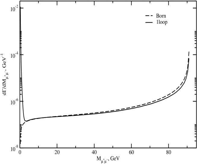
Figure 6: Invariant mass distribution of the $\mu^{+}\mu^{-}$ pair for the decay $Z\to\mu^{+}\mu^{-}\gamma(\gamma)$. Both the Born (dashed line) and the 1-loop (dotted line) results are shown.

The Coulomb peak, which is due to photon exchange in the Feynman one-loop diagram with a $\gamma Z\gamma$ three-boson vertex, is clearly seen.

4.3 $Z$ production channel $e\gamma\to eZ$

As can be seen from Table 8, we have again very good agreement between SANC and CompHEP predictions for the tree level and real photon emission cross sections of this process.

	$\sigma$, pb
$\sqrt{s}$, GeV	100	200	500	1000	2000
Born (SANC )	82.266(1)	23.716(1)	5.5747(1)	1.5343(1)	0.40648(1)
Born (CompHEP)	82.265(1)	23.716(1)	5.5747(1)	1.5343(1)	0.40647(1)
Hard (SANC )	4.012(1)	3.689(2)	1.368(1)	0.4986(6)	0.1682(3)
Hard (CompHEP)	4.014(0)	3.688(1)	1.364(1)	0.4973(6)	0.1678(3)

Table 8: Comparison of the Born cross sections for the $\gamma e^{-}\to Ze^{-}$ reaction and of the Hard cross sections for the $\gamma\mu^{-}\to Z\mu^{-}\gamma$ reaction (CompHEP input, $E_{\gamma}\geq 1$ GeV).

In Table 9 we present the results of our calculations for the channel $\gamma e^{-}\to Ze^{-}(\gamma)$ carried out with 10M statistics for the hard cross section for five energies and at each energy for two values of $\bar{\omega}$: $\bar{\omega}=10^{-5}\sqrt{s}/2$ (subscript 1) and $10^{-6}\sqrt{s}/2$ (subscript 2).

$\sqrt{s}$, GeV	200	500	1000	2000	5000
$\sigma^{\rm Born}$, pb	8.3381(3)	1.79168(0)	0.46840(0)	0.11842(0)	0.019007(0)
$\sigma^{\rm 1-loop}_{1}$, pb	8.7988(5)	1.9591(2)	0.52129(5)	0.13171(1)	0.02037(2)
$\sigma^{\rm 1-loop}_{2}$, pb	8.8002(9)	1.9593(2)	0.52131(6)	0.13168(1)	0.02037(3)
$\delta_{1}$, %	5.54(1)	9.35(1)	11.29(1)	11.23(1)	7.16(1)
$\delta_{2}$, %	5.54(1)	9.36(1)	11.30(1)	11.20(1)	7.15(2)

Table 9: Comparison of the Born and 1-loop cross sections of channel $\gamma e^{-}\to Ze^{-}(\gamma)$ calculated with different values of the soft/hard separation parameter $\bar{\omega}$.

The notation of the various contributions, $\sigma^{\rm Born}$ etc., is as in the previous case.

The cancellation of the $\lambda$-dependent terms was again checked on the algebraic level. The cancellation of the $\bar{\omega}$ dependence on the numerical level was tested as in the previous case. Comparing the corresponding values of $\sigma^{\rm 1-loop}$ and of $\delta$ we can see again that there is no change outside the statistical errors of the Monte Carlo integration.

The following cuts were imposed:

• CMS angular cuts for the Born cross section and for the contributions with Born-like kinematics: $\vartheta_{e,\,Z}\in[1^{\circ},179^{\circ}]$

• CMS angular cuts on the $Z$ boson and on the photon and a CMS energy cut on the electron for the hard contribution: for the event to be accepted, $\vartheta_{Z}$ and $\vartheta_{e}$ must lie in the interval $[1^{\circ},179^{\circ}]$, and the photon must have a CMS energy greater than $\bar{\omega}$.

The numbers in brackets give the statistical uncertainties of the last digit shown.

In Table 10 we show the comparison of the Born cross sections: the angular distributions $d\sigma/d\cos\vartheta_{e}$ and the cross sections integrated over the given angular intervals, as well as the 1-loop EW corrections $\delta$, produced by three programs: that of Ref. [24], Grace-loop [4] and SANC .

$\sqrt{s}$, GeV	$\vartheta$		Ref. [24]	Grace-loop	SANC
	$20^{\circ}$	$\sigma^{\rm Born}$, pb	0.3931		0.39308
		$\delta$, %	-5.96		-5.9556
	$90^{\circ}$	$\sigma^{\rm Born}$, pb	0.6491		0.64906
		$\delta$, %	-8.56		-8.5562
100	$160^{\circ}$	$\sigma^{\rm Born}$, pb	9.038		9.0383
		$\delta$, %	-10.00		-10.005
	$20^{\circ}<\theta<160^{\circ}$	$\sigma^{\rm Born}$, pb	13.051		13.051
		$\delta$, %	-9.04		-9.0389
	$1^{\circ}<\theta<179^{\circ}$	$\sigma^{\rm Born}$, pb	33.484		33.484
		$\delta$, %	-10.27		-10.273
	$20^{\circ}$	$\sigma^{\rm Born}$, pb	0.02898		0.028984
		$\delta$, %	-30.08		-30.079
	$90^{\circ}$	$\sigma^{\rm Born}$, pb	0.03598		0.035985
		$\delta$, %	-26.74		-26.744
500	$160^{\circ}$	$\sigma^{\rm Born}$, pb	0.4661		0.46607
		$\delta$, %	-23.05		-23.054
	$20^{\circ}<\theta<160^{\circ}$	$\sigma^{\rm Born}$, pb	0.7051	0.70515	0.70515
		$\delta$, %	-25.69	-25.689	-25.690
	$1^{\circ}<\theta<179^{\circ}$	$\sigma^{\rm Born}$, pb	1.770	1.7696	1.7697
		$\delta$, %	-22.31	-22.313	-22.313
	$20^{\circ}$	$\sigma^{\rm Born}$, pb	0.001869		0.0018688
		$\delta$, %	-41.57		-41.575
	$90^{\circ}$	$\sigma^{\rm Born}$, pb	0.002334		0.0023340
		$\delta$, %	-41.98		-41.981
2000	$160^{\circ}$	$\sigma^{\rm Born}$, pb	0.03094		0.030942
		$\delta$, %	-33.99		-33.994
	$20^{\circ}<\theta<160^{\circ}$	$\sigma^{\rm Born}$, pb	0.04620	0.046201	0.046201
		$\delta$, %	-39.53	-39.529	-39.529
	$1^{\circ}<\theta<179^{\circ}$	$\sigma^{\rm Born}$, pb	0.1170	0.1170	0.11697
		$\delta$, %	-30.84	-30.845	-30.845

Table 10: Triple comparison of the Born cross section and of the correction $\delta=\sigma^{\rm 1-loop}/\sigma^{\rm Born}-1$ for channel $\gamma e^{-}\to Ze^{-}(\gamma)$ (Ref. [24] input, $E_{\gamma}=0.025\sqrt{s}$ GeV).

We have excellent agreement between these three results. Note that in this table the results taken from the literature were given there without statistical errors. The statistical errors of numbers obtained with SANC are in the digits beyond those shown.

5 Conclusions

In this paper we describe the implementation of the complete one-loop EW calculations, including hard bremsstrahlung contributions, for the process $f_{1}\bar{f}_{1}ZA\to 0$ into the SANC framework. The calculations were done using a combination of analytic and Monte Carlo integration methods which make it easy to calculate a variety of observables and to impose experimental cuts. We have presented analytical expressions for the covariant amplitudes of the process and the helicity amplitudes for three different cross channels: $Z$ boson production $f_{1}\bar{f}_{1}\to Z\gamma$ and $f_{1}\gamma\to f_{1}Z$, and for the decay $Z\to f_{1}\bar{f}_{1}\gamma$. To be assured of the correctness of our analytical results, we observe the independence of the form factors on gauge parameters (all calculations were done in $R_{\xi}$ gauge), the validity of the Ward identity for the covariant amplitudes. We have compared our numerical results for these processes with other independent calculations. The Born level and the hard photon contrubutions of all three channels were checked against CompHEP package and we found a very good agreement except for the annihilation channel at high energies. For the channel $\gamma e^{-}\to Ze^{-}(\gamma)$, the comparison of the SANC EW NLO predictions with the results of Refs. [24, 4] has shown an excellent agreement in a wide range of CMS energies and final electron scattering angles.

The results presented lay a base for subsequent extensions of calculations in the annihilation channel appropriate to the process $pp\to XZ\gamma$ at hadron colliders.

Acknowledgements. This work is partly supported by INTAS grant $N^{o}$ 03-51-4007
and by the EU grant mTkd-CT-2004-510126 in partnership with the CERN Physics Department and by the Polish Ministry of Scientific Research and Information Technology grant No 620/E-77/6.PRUE/DIE 188/2005-2008 and by Russian Foundation for Basic Research grant $N^{o}$ 07-02-00932.

WvS is indebted to the directorate of the Dzhelepov Laboratory of Nuclear Problems, JINR, Dubna for the hospitality extended to him during September 2007.

References

• [1] R. Mertig, M. Bohm, and A. Denner, Comput. Phys. Commun. 64 (1991) 345–359.
• [2] T. Hahn and M. Perez-Victoria, Comput. Phys. Commun. 118 (1999) 153–165, hep-ph/9807565.
• [3] T. Hahn, Comput. Phys. Commun. 140 (2001) 418–431, hep-ph/0012260.
• [4] G. Belanger et al., Phys. Rept. 430 (2006) 117–209, hep-ph/0308080.
• [5] A. Andonov et al., Comput. Phys. Commun. 174 (2006) 481–517, hep-ph/0411186.
• [6] Dubna — http://sanc.jinr.ru, CERN — http://pcphsanc.cern.ch (2007).
• [7] D. Bardin, S. Bondarenko, L. Kalinovskaya, G. Nanava, and L. Rumyantsev, Eur. Phys. J. C52 (2007) 83–92, hep-ph/0702115.
• [8] D. Bardin et al., hep-ph/0506120.
• [9] D0 Collaboration, V. M. Abazov et al., Phys. Lett. B653 (2007) 378–386, arXiv:0705.1550 [hep-ex].
• [10] D0 Collaboration, V. M. Abazov et al., Phys. Rev. Lett. 95 (2005) 051802, hep-ex/0502036.
• [11] CDF II Collaboration, D. Acosta et al., Phys. Rev. Lett. 94 (2005) 041803, hep-ex/0410008.
• [12] U. Baur and D. L. Rainwater, Phys. Rev. D62 (2000) 113011, hep-ph/0008063.
• [13] S. Haywood et al., hep-ph/0003275.
• [14] S. Atag and I. Sahin, Phys. Rev. D70 (2004) 053014, hep-ph/0408163.
• [15] R. Walsh and A. J. Ramalho, Phys. Rev. D65 (2002) 055011.
• [16] E. Accomando, A. Denner, and C. Meier, Eur. Phys. J. C47 (2006) 125–146, hep-ph/0509234.
• [17] T. G. Rizzo, Phys. Rev. D54 (1996) 3057–3064, hep-ph/9602331.
• [18] S. Atag and I. Sahin, Phys. Rev. D68 (2003) 093014, hep-ph/0310047.
• [19] M. A. Perez and F. Ramirez-Zavaleta, Phys. Lett. B609 (2005) 68–72, hep-ph/0410212.
• [20] B. Ananthanarayan, S. D. Rindani, R. K. Singh, and A. Bartl, Phys. Lett. B593 (2004) 95–104, hep-ph/0404106.
• [21] M. Capdequi Peyranere, Y. Loubatieres, and M. Talon, Nuovo Cim. A90 (1985) 363.
• [22] F. A. Berends, G. J. H. Burgers, and W. L. van Neerven, Phys. Lett. B177 (1986) 191.
• [23] A. Denner and S. Dittmaier, hep-ph/9308360.
• [24] A. Denner and S. Dittmaier, Nucl. Phys. B398 (1993) 265–284.
• [25] G. P. Lepage, J. Comput. Phys. 27 (1978) 192.