The Chemical Enrichment History of the Large Magellanic Cloud

Abstract

Ca II triplet spectroscopy has been used to derive stellar metallicities for individual stars in four LMC fields situated at galactocentric distances of 3°, 5°, 6° and 8° to the north of the Bar. Observed metallicity distributions show a well defined peak, with a tail toward low metallicities. The mean metallicity remains constant until 6° ([Fe/H]$\sim$-0.5 dex), while for the outermost field, at 8°, the mean metallicity is substantially lower than in the rest of the disk ([Fe/H]$\sim$-0.8 dex). The combination of spectroscopy with deep CCD photometry has allowed us to break the RGB age–metallicity degeneracy and compute the ages for the objects observed spectroscopically. The obtained age–metallicity relationships for our four fields are statistically indistinguishable. We conclude that the lower mean metallicity in the outermost field is a consequence of it having a lower fraction of intermediate-age stars, which are more metal-rich than the older stars. The disk age–metallicity relationship is similar to that for clusters. However, the lack of objects with ages between 3 and 10 Gyr is not observed in the field population. Finally, we used data from the literature to derive consistently the age–metallicity relationship of the bar. Simple chemical evolution models have been used to reproduce the observed age–metallicity relationships with the purpose of investigating which mechanism has participated in the evolution of the disk and bar. We find that while the disk age–metallicity relationship is well reproduced by close-box models or models with a small degree of outflow, that of the bar is only reproduced by models with combination of infall and outflow.

1 Introduction

Despite decades of work, there are still significant gaps in our knowledge of the LMC’s star formation and chemical enrichment histories (Olszewski et al., 1996). This is motivated in part by the vastness of its stellar populations and to our limitations in observing sizable samples of stars. The age distribution of star clusters is relatively well known (e.g. Geisler et al., 1997): there is an age interval between 10 and 3 Gyr with almost no clusters. This so-called age-gap may also correspond to an abundance gap (Olszewski et al., 1991), since the old clusters are metal-poor while the young ones are relatively metal-rich. The star formation history (SFH) of field stars is much less precisely known. Studies using HST data in small fields, suggest that the SFH of the LMC disk has been more or less continuous, with some increase in the star formation rate (SFR) in the last few Gyr (e.g. Smecker-Hane et al., 2002; Castro et al., 2001; Holtzman et al., 1999). This contrasts with previous results (based on much shallower data), which found a relatively young age (a few Gyr) for the dominant LMC population (Hardy et al., 1984; Bertelli et al., 1992; Westerlund, Linde, & Lynga, 1995; Vallenari et al., 1996). The SFH of the LMC can now be studied using sufficiently deep ground-based data (e.g. reaching the oldest main-sequence turn-off with good photometric precision) in large areas and in different positions of the galaxy (e.g. Gallart et al., 2004, 2007, hereafter Paper I).

Less is known about the LMC chemical enrichment history. The age–metallicity relation (AMR) normally used for the LMC is defined by star clusters (e.g. Olszewski et al., 1991; Geisler et al., 1997; Bica et al., 1998; Dirsch et al., 2000). All works based on clusters obtain similar results. The mean metallicity jumps from [Fe/H] $\sim-1.5$ for the oldest clusters to [Fe/H] $\sim-0.5$ for the youngest ones. There were no studies on the field population AMR until the last decade. Dopita et al. (1997), from a study of $\alpha$-elements in planetary nebulae, obtained a result qualitatively similar to that found in the clusters although only ten objects were used. Later, Bica et al. (1998), using Washington photometry, and Cole, Smecker-Hane, & Gallagher (2000) and Dirsch et al. (2000), using Ströngrem photometry, obtained the metallicity of RGB stars in different positions of the LMC. Cole, Smecker-Hane, & Gallagher (2000) also observed 20 stars with the infrared CaII triplet (CaT). All of them found that the age-gap observed in the clusters is not found in the field population. More recently, Cole et al. (2005) have obtained stellar metallicities for almost 400 stars in the bar of the LMC, also using CaT lines. The metallicity for each star has been combined with its position in the color–magnitude diagram (CMD) to estimate its age. The obtained AMR shows a similar behavior to that of the clusters for the oldest population. However, while for the clusters the metallicity has increased over the last 2 Gyr, this has not happened in the bar. Finally Gratton et al. (2004) measured the metallicity of about 100 bar RR Lyrae, obtaining an average metallicity of [Fe/H] $=-1.48$.

Another point that it is necessary to investigate is the presence, or not, of an abundance gradient in the LMC. From observations of clusters, Olszewski et al. (1991) and Santos Jr. et al. (1999) found no evidence for the presence of a radial metallicity gradient in the LMC. The only evidence for a radial metallicity gradient in the LMC cluster system was reported by Kontizas, Kontizas, & Michalitsiano (1993) based on six outer LMC clusters ($\geq$ 8 kpc). Hill, Andrievsky, & Spite (1995) were the first to report evidences of a gradient in the field population from high-resolution spectroscopy, using a sample of nine stars in the bar and in the disk. They found that the bar is on average 0.3 dex more metal-rich than the disk population, but the disk stars studied are located within a radius of 2°. Subsequent work by Cioni & Habing (2003), detected that the C/M ratio between number of asymptotic giant branch stars of spectral types C and M increased when moving away from the bar and within a radius of 6$\fdg$7. As the C/M ratio is anticorrelated with metallicity, this increment implies a decrease in metallicity. Finally, an outward radial gradient of decreasing metallicity was also found by Alves (2004) from infrared CMD using the 2MASS survey.

We have obtained deep photometry with the Mosaic II CCD Imager on the CTIO 4m telescope in four disk fields at different distances from the center of the LMC (RA=5^h23^m34$\fs$5, $\delta$=-69$\arcdeg$45’22“) with a quality similar to that obtained by HST in more crowded areas (see Paper I). The position of these fields, together with a description of their CMDs, are presented in Paper I, and detailed SFHs will be published in forthcoming papers. In the present investigation we focus on obtaining stellar metallicities for a significant number of individual RGB stars in these four fields using spectra obtained with the HYDRA spectrograph at the CTIO 4m telescope. In Section 2 we present our target selection. The observations and data reduction are presented in Section 3. The radial velocities of the stars in our sample are obtained in Section 4. In Section 5 we discuss the calculation of the CaT equivalent widths and the determination of metallicities. Section 6 presents the method used to derive ages for each star by combining the information on their metallicity and position on the CMD. The analysis of the data is presented in Section 7, where the possible presence of a kinematically hot halo is discussed and the AMR and the SFH in each of our fields are described and compared. In the final section, the AMRs are compared to theoretical models and conclusions are drawn about the chemical evolution of the LMC.

2 Target Selection

Our starting point are deep CMDs of four $36^{\prime}\times 36^{\prime}$ fields located $\sim$3$\arcdeg$, 5$\arcdeg$, 6$\arcdeg$ and 8$\arcdeg$ from the LMC center, which are presented and discussed in Paper I. All fields are located north of the LMC bar, and their CMDs reach the oldest main-sequence turn-offs. A clear gradient exists in the amount of intermediate-age and young populations from the inner to the outermost fields, in the sense that the young population is more prominent in the inner parts (see Paper I for a more detailed discussion).

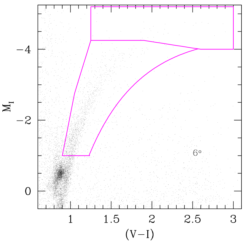
Figure 1: CMD of the RGB region of the field situated at 6° from the LMC center. The regions used to select stars to be observed spectroscopically are shown.

In each field we have selected the stars to be observed with HYDRA in two windows in the CMD, which are plotted in Figure 1. The bluest color limit has been selected to avoid upper red-clump and red supergiant stars and the lower magnitude limit to avoid including red-clump stars in the spectroscopic sample. The blue edge of the window is sufficiently blue to ensure that no metal poor stars would be excluded (the position of the blue ridge corresponds approximately with the position of $\sim$2 Gyr old stars with [Fe/H]=-3). Similarly, the opposite edge is sufficiently red so that even old stars with solar metalicities, or even higher, fit within the box. These selected stars have been ordered from the brightest to the faintest ones, with no color restriction. This list has been used as input for the configuration task of the instrument, which tries to optimize the number of allocated fibers. The first stars in the list, the brightest ones, have priority over the others.

3 Observations and Data Reduction

The observations were carried out in two different runs, in December 2002 and in January 2005, at the CTIO 4 m telescope with the HYDRA multifiber spectrograph. We used the KPGLD grating, which provides a central wavelength of 8500 Å, and a OG590 order-blocking filter. The physical pixels were binned 2 $\times$ 1 in the spectral direction yielding a dispersion of 0.9 Å/pix. HYDRA has a field of view of about 40 arcmin, which on account of the high density of stars in our fields, allowed us to observe more than 100 stars in each configuration, with the 140 available fibers. Because of technical problems and bad weather, on our first run we were able to observe only two configurations located at 5$\arcdeg$ and 8$\arcdeg$ respectively. In the more successful second run, one fiber configuration in each field was observed except for the closest one, where we observed two configurations. Stars in two globular clusters, NGC 4590 and NGC 3201, were also observed. Those in the first were used as radial velocity standards, but also to compare the equivalent widths determined through the present set-up with those setups used for the cluster observations reported in Carrera et al. (2007, hereafter Paper II). Since the differences were negligible (see Figure 1 of paper II), the second cluster was included in the calibration of the CaT as metallicity indicator. We concluded that the LMC equivalent widths obtained with the present observational setup could be directly transformed into [Fe/H] using the calibration in paper II. Equivalent widths, magnitudes and radial velocities for the 702 stars observed in the LMC are listed in Table 1.

The data reduction was done following the procedure described in Knut Hydra notes. First, cosmic rays were removed from the images using the IRAF Laplacian edge-detection routine (van Dokkun, 2001). All images were then bias- and overscan-subtracted, and trimmed. Flat exposures were taken during the day with a diffusing screen installed in the spectrograph to obtain the so-called ”milk-flat”, which is used to correct the effect of the different sensitivities among pixels. It was applied to all images using ccdproc. The spectra were extracted, flat-field corrected (see bellow), and calibrated in wavelength using dohydra, a program developed specifically to reduce the data obtained with this spectrograph. The lamp flats acquired at the beginning of each configuration were used to define and trace each aperture. The sky flats were used to eliminate the residuals after the flat-field correction with the milk-flat. Arcs, obtained before and after each configuration, were used for wavelength calibration.

Dohydra can also perform sky subtraction. However, we noticed that after sky subtraction, there remained significant sky line residues. We therefore developed our own procedure to remove the contribution of the sky lines from the object spectra. For a given configuration, we obtain an average high signal–to–noise ratio (S/N) sky spectrum from all fibers placed on the sky. Before subtracting this averaged sky from each star spectrum, we need to know the relation between the intensity of the sky in each fiber (which varies from fiber to fiber owing to the different fiber responses) and the average sky. This relation is used as a weight (which may depend on wavelength) that multiplies the average sky spectrum before subtracting it from each star. Our task minimizes the sky line residuals over the whole spectral region considered and allows very accurate removal of the sky emission lines. An example of raw, sky and final object is shown in Figure 2.

We obtained between three and four exposures of 2700 s in each configuration. To minimize the contribution of residuals arising from cosmic rays and bad pixels, all spectra of the same object were combined. Finally, each object spectrum was normalized with the continuum task by fitting a polynomial, making sure to exclude all absorption lines in our wavelength range, such as the CaT lines themselves.

4 Radial Velocities

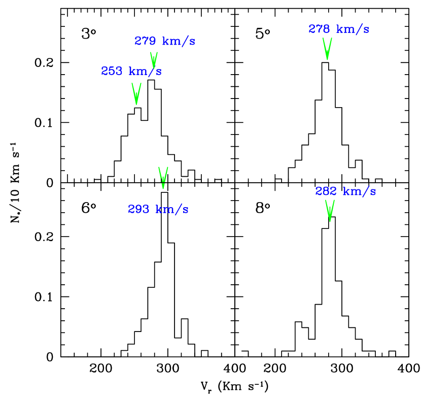
Figure 3: Radial velocity distributions of our four LMC fields. The mean value of each distribution is shown in each panel, and its position is marked with an arrow. Note that there are two peaks in the field situated at 3°.

Our main purpose in obtaining radial velocities for our program stars is to reject possible foreground objects. However, radial velocities can provide more useful information, as discussed in depth in Section 7.1. The radial velocities were calculated with the fxcor task in IRAF, which performs the cross-correlation described by Tonry & Davis (1979) between the spectra of the target and selected templates of known radial velocities. As templates, we used three stars in the globular cluster NGC 4590 (M68) with radial velocities obtained by Geisler et al. (1995). The final radial velocities for all the stars in our sample were obtained as the average of the velocities obtained with the three templates, weighted by the width of the corresponding correlation peaks. Radial velocity histograms for each field are plotted in Figure 3. A Gaussian function was fitted in order to obtain the central peak and the $\sigma$ of each distribution (values listed in Table 2). The velocity distribution of the field located 3° from the center shows two peaks, which are marked in Figure 3. Stars with radial velocity in the range 170 $\leq V_{r}\leq$ 380 km s^-1 (Zhao et al., 2003) are considered LMC members. Only about 20 stars in each configuration of the instrument have been excluded based on their radial velocity. These results are discussed in depth in Section 7.1.

5 CaT Equivalent Widths and Metallicity Determination

The metallicity of the RGB stars is obtained following the procedure described in Paper II. In short, the equivalent width is the line area normalized to the continuum. The continuum is calculated from the linear fit to the mean value of each bandpass, defined to obtain the continuum position. We have used the continuum and line bandpasses defined by Cenarro et al. (2001), which are listed in Table 3. The equivalent widths are calculated from profile fitting using a Gaussian plus a Lorentzian. This combination provides the best fit to line core and wings as discussed in Paper II. The CaT index is defined as the sum of the equivalent widths of the three CaT lines, denoted as $\Sigma Ca$. The $\Sigma Ca$ calculated for each observed star and its uncertainty are given in Table 1, together with the star magnitude and radial velocity. The reduced equivalent width, $W^{\prime}_{I}$, for each star has been calculated as the value of $\Sigma Ca$ at M_I=0, using the slope obtained in Paper II for the calibration clusters in the M_I–$\Sigma Ca$ plane ($\beta_{I}$ = $-0.611$ Åmag^-1).

In Paper II we obtained relationships between the reduced equivalent widths, $W^{\prime}_{V}$ and $W^{\prime}_{I}$, and metallicity, on the Zinn & West (1984), Carretta & Gratton (1997, hereafter CG97) and Kraft & Ivans (2003) scales. In this case, we will only use the relationships obtained on the CG97 metallicity scale, because it is the only one in which the metallicities of our open and globular calibration clusters have been obtained in a homogeneous way from high-resolution spectroscopy.

In order to verify that the $V$ and $I$ relationships give similar results, we have applied both to obtain the metallicities of the stars observed in the field located at 5°. The differences are on average $-$0.01 dex, and never larger than 0.15 dex for stars with $(V-I)\leq$ 2.5. For stars with colors larger than this, the differences are on average 0.2 dex and never get above 0.35 dex. The calibration stars used in Paper II have $(V-I)<2.5$, so the metallicities calculated for the reddest stars are necessarily extrapolations of the relationships. On average, the relationship based on M_I yields metallicities slightly lower than those obtained from M_V, but always within the uncertainties. In what follows we will use the relationship based on M_I, because: i) the photometric accuracy in $I$ is slightly better than in $V$, especially for the reddest stars on the RGB; ii) the RGB is better resolved in the $I$ band; and iii) from a theoretical point of view (Pont et al., 2004), it is likely that the relationship based on M_I is less sensitive to age. In short, then, the metallicity for each star is given by:

$$[Fe/H]_{CG97}=-2.95+0.38\Sigma Ca+0.23M_{I}$$ (1)

Binarity could affect the derived metallicity only in the unlikely case of the two stars in the system being RGB stars of a very similar mass. In this case the system would be $\sim$0.7 mag brighter than a single star. As the binarity might not affect the equivalent width of the CaT lines, the derived metallicity would be lower by $\sim$0.4 dex than the actual metallicity.

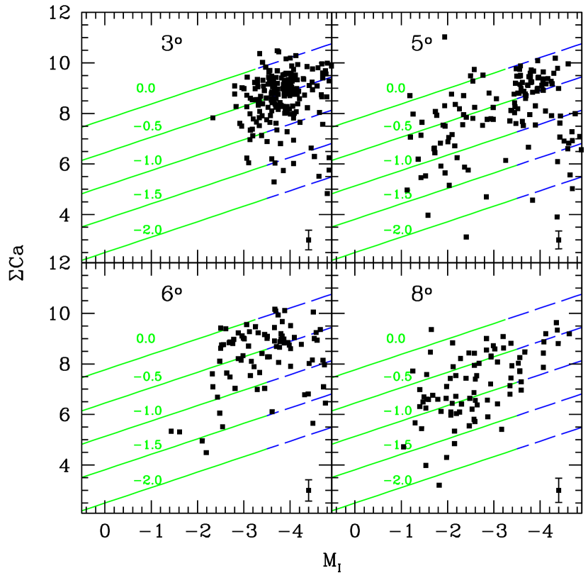
Figure 4: Position in the M_I–$\Sigma$Ca plane of LMC stars for which membership has been confirmed from their radial velocity. The typical $\Sigma Ca$ error is shown in the bottom right corner of each panel. Isometallicity lines have been plotted for reference. The solid part of each line is the magnitude interval covered by the cluster stars used for the calibration (see Paper II). The dashed part is the region in which the calibration is extrapolated.

Figure 4 shows the position of LMC radial velocity member stars in the M_I–$\Sigma$Ca plane for our four fields, from the innermost one (top left) to the outermost field (bottom right). The star with $\Sigma Ca$ = 11 and M_I = $-$2 in the field situated at 5$\arcdeg$ has a well measured $\Sigma Ca$ and radial velocity V_r = 264 km s^-1 (the mean V_r of the sample is 278 $\pm$ 20 km s^-1), so it seems to be an LMC RGB star with unusually large metallicity. However, a reliable metallicity cannot be obtained with the present calibration, which is only valid for [Fe/H] $\leq$ +0.47. The extrapolation of our calibration gives [Fe/H] = +0.72 $\pm$ 0.4 for this star.

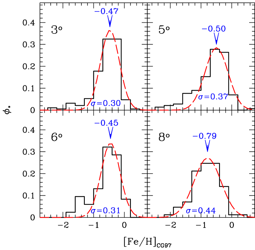
Figure 5: Metallicity distributions for the four fields in our sample. A Gaussian has been fitted to each distribution in order to obtain its mean and dispersion. The values obtained are shown in each panel.

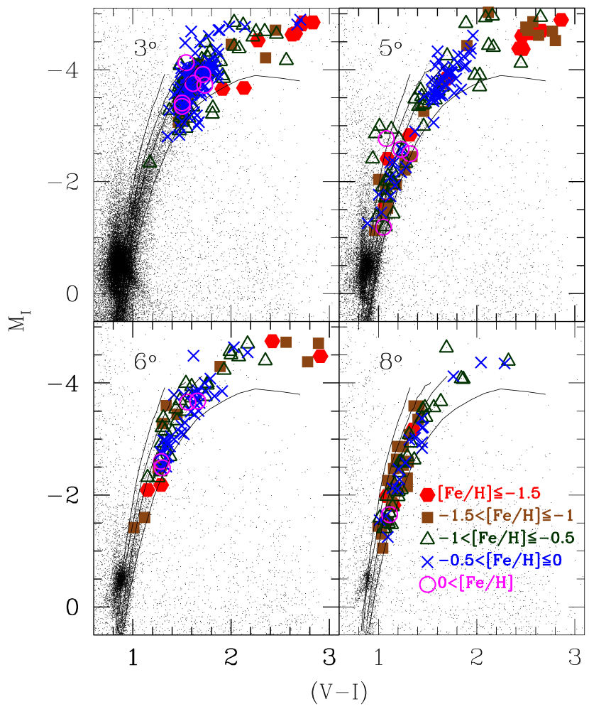
Figure 6: Position of the observed star in the color-magnitude diagram. Different metallicity intervals are represented by different symbols, as indicated in the label. Solid lines are the fiducial sequences of four globular clusters (from right to left: NGC 104: [Fe/H] = $-0.78$; NGC 5904: [Fe/H] =$-1.12$; NGC 5272: [Fe/H] = $-1.34$ and NGC 6341: [Fe/H] = $-2.16$).

The metallicity distribution of each field is shown in Figure 5 and will be discussed in extenso in Section 7.2. In Figure 6 the observed stars have been plotted in the color–magnitude diagram employing different symbols as a function of their metallicity. It is important to highlight that there is no correlation between the metallicity of the stars and their position in the color–magnitude diagram, as was also found in other galaxies (e.g. Pont et al., 2004; Cole et al., 2005; Koch et al., 2006). This shows once more that the metallicities derived from the position of the stars in the RGB are unreliable in systems with complex SFHs.

6 Determination of stellar ages

For a given age, the position of the RGB on the color–magnitude diagram depends mainly on metallicity in the sense that more metal-rich stars are redder than more metal-poor ones. At the same time, for a fixed metallicity, older stars are also redder than younger ones. If we take into account the logical assumption that younger stars are also more metal-rich, age may partly counteract the effect of metallicity. The combination of both effects is the well known RGB age–metallicity degeneracy, which sets a limit on the amount of information that can be retrieved from the RGB using only photometric data. However, if stellar metallicities are obtained independently from another source, such as spectroscopy, we should in principle be able to break the age–metallicity degeneracy. Pont et al. (2004) and Cole et al. (2005) have derived stellar ages from isochrones for stars whose metallicity had been previously obtained from low-resolution spectroscopy. In our case, instead of directly comparing the position of the star in the CMDs with isochrones, we have obtained a relation for the age as a function of color, magnitude and metallicity from a synthetic CMD. This allows to easily obtain ages for the large number of stars in our sample.

The reference synthetic CMD has been computed using IAC-STAR (Aparicio & Gallart, 2004). Its main input parameters are the SFR and the chemical enrichment law, as a function of time. Since we are interested in a general relation, we have chosen a constant SFR for the whole range of ages (13 $\geq$ (Age/Gyr) $\geq$ 0) and a chemical enrichment law such that a star of any age can have any metallicity in the range $-2.5\leq$ [Fe/H] $\leq$ +0.5. Both the constant SFR and the chemical enrichment law ensure that there is no age or metallicity bias. We have computed two synthetic CMDs, one using the BaSTI stellar evolution library (Pietrinferni et al., 2004) and another using the Padova library (Girardi et al., 2002) respectively. The ranges of ages and metallicities covered, as well as other important features of each library are listed in Table 1 of Gallart, Zoccali & Aparicio (2005).

Since the uncertainty of the age assigned by stellar evolution models to bright AGB stars is large, we will only compute ages for RGB and AGB stars fainter than the RGB tip (M${}_{I}\sim$-4 in Figure 1) . We have chosen the synthetic stars in the box below the tip of the RGB shown in Figure 1. We have computed a polynomial relationship which gives the age as a function of [Fe/H] $\equiv$  log(Z/Z_⊙), (V-I) and M_V. In order to minimize the $\sigma$ and to improve the correlation coefficient of the relation, different linear, quadratic and cubic terms of each observed magnitude have been added. When the addition of a term did not improve the relation we rejected it. The best combination of these parameters is in the form of Equation 2 and the values obtained for each stellar evolution library are shown in Table 4. Note that each stellar evolution library has its own age scale, and some differences might exist among them.

$$log(age)=a+b(V-I)+cM_{V}+d[Fe/H]+f(V-I)^{2}+g[Fe/H]^{2}+h(V-I)^{3}$$ (2)

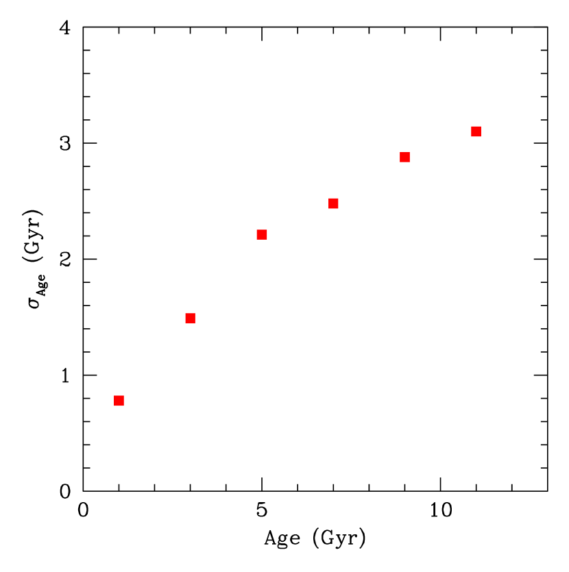
Figure 7: Uncertainty in the age calculated using Equation 2 obtained from the BaSTI stellar evolution models. See text for details.

The uncertainties of each term on Equation 2 are given in Table 4. However, the way in which they propagate into the error of the age is complex. For this reason a Monte Carlo test has been performed to estimate age errors. The synthetic stellar population computed from BaSTI stellar evolution models has been used to this purpose. That based on the Padua library would have produced similar results. The test consists in computing, for each synthetic star, several age values for stochastically varying $[Fe/H]$, $(V-I)$ and $M_{V}$ according to a gaussian probability distribution of the corresponding $\sigma$ ($\sigma_{[Fe/H]}\sim$0.15 dex; $\sigma_{(V-I)}\sim$0.001 and $\sigma_{M_{V}}\sim$ 0.001). The $\sigma$ value of the obtained ages provide an estimation of the age error when Equation 2 is used. The values obtained for different age intervals are shown in Figure 7. The error increases for older ages.

We have also investigated the accuracy with which the age of a real stellar population is measured. The stars in open and globular clusters in Paper II, which ages are independently known, are used for this purpose. We adopt the ages estimated by Salaris & Weiss (2002) and Salaris, Weiss, & Percival (2004), which are in a common scale, for a globular and open clusters, respectively. They are listed in Table 1 of Paper II.

The age of each cluster star has been estimated from Equation 2 assuming the distance modulus and reddening listed in Paper II. The metallicity of each star has been calculated following the same procedure as for the LMC stars (see Section 5). The age of each cluster has been obtained as the mean age derived from all the stars in each cluster and the quoted uncertainty is the standard deviation of this mean. Ages derived for each cluster from the BaSTI and Padova relationships in Table 4, versus the reference values for each cluster, have been plotted in Figure 8. The relationships saturate for ages older than 10 Gyr because differences of 1 or 2 Gyr produce only negligible variations of position in the CMD. In both cases, the age of clusters younger than 10 Gyr are well reproduced. Differences between the age derived with each model and the reference value are within the error bars, with the exception of cluster NGC 6819 for the BaSTI relationship. The large errorbar of the youngest cluster, NGC 6705, is due to the fact that the stars observed in this cluster are fainter that the synthetic stars used to derive the relationships. Therefore, we are extrapolating the relations to obtain the age of this cluster. As both models produce similar values, we adopted for simplicity the relationships derived from the BaSTI stellar library (Pietrinferni et al., 2004).

7 Analysis

7.1 Stellar kinematics of the LMC

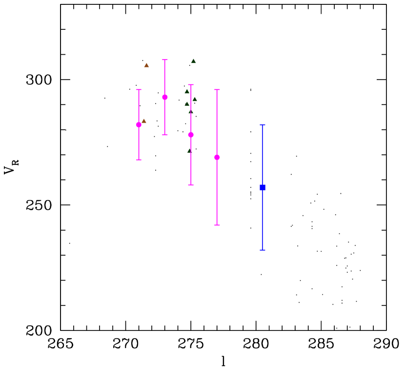
Figure 9: Radial velocities for carbon stars from Kunkel et al. (1997) in the band $-36\arcdeg\leq b\leq-33\arcdeg$. The triangles are the carbon stars in our fields at 5° and 8°. The filled square represents the data from Cole et al. (2005) for the bar. The filled dots are our data listed in Table 2. The error bars represent the dispersions of the velocity distributions.

In Figure 9 we have plotted the mean of the velocity distribution for each field (including the Cole et al., 2005, bar field) as a function of its Galactic longitude. The mean velocity changes from field to field due to the disk rotation of the LMC. The radial velocities of carbon stars derived by Kunkel et al. (1997) have also been plotted. Our data are in good agreement with their result, which is consistent with the presence of a rotational disk.

If a classical Milky Way-like halo existed in the LMC (i.e. old, metal-poor and with high velocity dispersion), a dependency between the velocity dispersion and metallicity/age of the stars in our sample might be observed. The first evidence of the presence of a kinetically hot spheroidal population was reported by Hughes, Wood, & Reid (1991). They found that the LMC long period variables, related to an old stellar population, have a high velocity dispersion (33 km s^-1), with a low rotational component. Minniti et al. (2003) measured the kinematics of 43 RR Lyrae stars in the inner regions of the LMC and found that the velocity dispersion of these stars is 53 $\pm$ 10 km s^-1, which they associated with the presence of a kinematically hot halo populated by old metal-poor stars. Some studies of the intermediate-age and old populations have found that the velocity dispersion increases with age (e.g. Hughes, Wood, & Reid, 1991; Schommer et al., 1992; Graff et al., 2000). In fact Graff et al. (2000), using C stars, have found the stars of the disk belong to two populations: a young disk population containing 20% of stars with a velocity dispersion of 8 km s^-1, and an old disk population containing the remaining stars with a velocity dispersion of 22 km s^-1.

We can check the presence of a hot halo with our sample stars. Assuming that stars with similar metallicities are of similar ages (see below), a possible dependency of velocity dispersion with metallicity could indicate whether different stellar populations have different kinematics.

The procedure has been the follow up. The mean velocity in each field has been subtracted from the radial velocity of each star to eliminate the rotational component of the disk. The total metallicity range has been divided into three bins. The velocity dispersion of stars in each metallicity bin is listed in Table 5 and plotted in Figure 10. The velocity dispersion for old and metal-poor stars, 26.4 km s^-1, is slightly smaller than the value found by Hughes, Wood, & Reid (1991) for the old long period variables ($\sigma$=33 km s^-1) and significantly smaller than the dispersion found in RR Lyrae stars ($\sigma\sim$53 km s^-1, Minniti et al., 2003). Cole et al. (2005) found a velocity dispersion of $\sigma$ = 40.8 km s^-1 for the most metal-poor stars in the bar, which is also higher than the value found here. The metal-poor stars in our sample seem to be members of the thick disk instead of the halo. In short, from our data we have found no clear evidence for the presence of a kinematically hot halo populated by old stars.

7.2 Metallicity distribution

The metallicity distribution for each field is shown in Figure 5. We have fitted a Gaussian to each one in order to obtain its mean value and dispersion (Table 6). The mean value is constant at [Fe/H]$\sim$-0.5 dex up to 8$\arcdeg$, where the mean metallicity decreases by about a factor of two ([Fe/H]=-0.8 dex). All metallicity distributions are similar. They show a clear peak with a tail toward low metallicities. We complement our sample with the results by Cole et al. (2005), who derived stellar metallicities in the bar in a similar way as here. As demonstrated in Paper II, their CaT index is equivalent to ours. Using their measurements of the $\Sigma Ca$ we can calculate the metallicities from Equation 1. We have also fitted a Gaussian to the resulting bar metallicity distribution to obtain its mean value. On average, the bar is slightly more metal-rich than the inne disk [Fe/H]$\sim$-0.4 dex).

7.3 Age–metallicity relationships

To understand the nature of the observed metallicity distributions, and to join insight on SFR and the chemical enrichment history of the LMC fields, we have estimated the age of each star in our sample following the procedure described in Section 6. These individual age determinations have a much larger uncertainty than the metallicity calculations. However, they are still useful because we are interested in the general trend rather than in obtaining precise values for individual stars.

We assumed that the oldest stars have the same age as the oldest cluster in our galaxy, for which we adopt 12.9 Gyr (NGC 6426, Salaris & Weiss, 2002). This agrees with a 13.7$\pm$0.2 Gyr old Universe (Spergel et al., 2003) where the first stars formed about 1 Gyr after the Big Bang. Another important point is the youngest age that we can find in our sample. According to stellar evolution models (Pietrinferni et al., 2004), we do not expect to find stars younger than 0.8 Gyr in the region of the RGB where we selected our objects. However, application of Equation 2 may result in ages younger than this value. To avoid this contradiction, and taking into account that the age determination uncertainty for the younger stars is about 1 Gyr, we assigned an age of 0.8 Gyr to those stars for which Equation 2 gives younger values. Finally, as the relationships used to estimate the age have been calculated for stars below the tip of the RGB, only stars fainter than this point have been used.

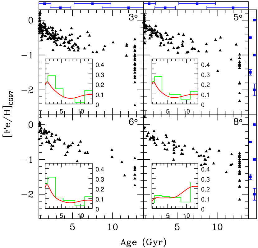
Figure 11: Age–metallicity relationships for the four LMC fields in our sample. Inset panels show the age distribution computed taking into account (solid line) and not (histogram) the age determination uncertainties. The top panel show the age error in each interval. The left panels show the metallicity error.

The age of each star versus its metallicity (i.e. the AMR) has been plotted in Figure 11 for each field. The many stars with the same age that appear both at the old (12.9 Gyr) and young (0.8 Gyr) limits are the consequence of the boundary conditions imposed on the ages, and the exact values should not be taken at face value. The age error in each age interval, computed in Section 6, is indicated in the top panel. The age distribution for each field has been plotted in inset panels. The histogram is the age distribution without taking into account the age uncertainty. The solid line is the same age distribution computed by taking into account the age error. To do this, a Gaussian probability distribution is used to represent the age of each star. The mean and $\sigma$ of the Gaussian are the age obtained for the star and its error, respectively. The area of each Gaussian is unity. In stars near the edges, the wings of the distributions may extend further than the age physical limits. In such cases, we truncated the wing and rescaled the rest of the distribution such that the area remains unity.

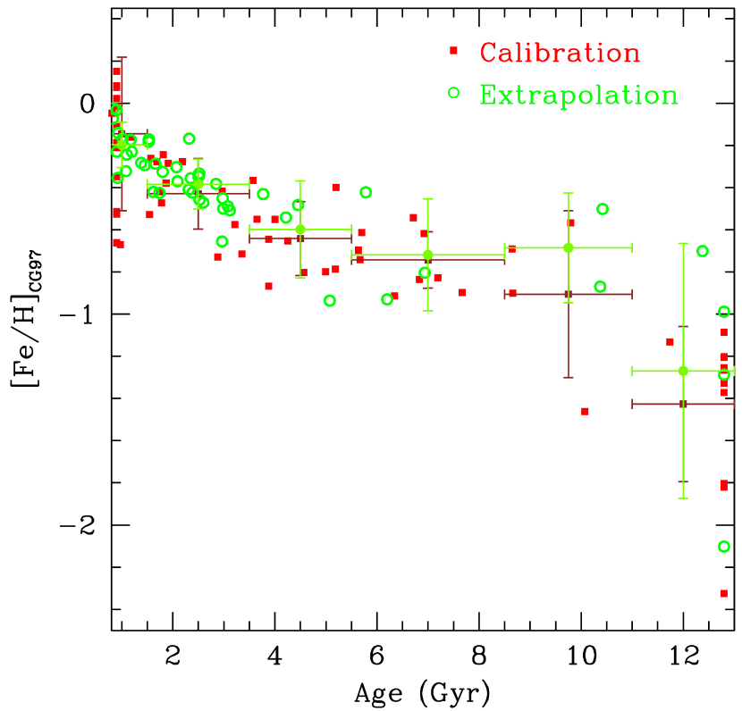
Figure 12: AMR of the field situated at 5° for different star groups. Squares: objects with magnitudes in the range of the M_I–$\Sigma Ca$ calibration obtained in Paper II; open circles: objects in the same field with magnitudes brighter than the cluster calibration stars. The corresponding average metallicity and dispersion in different age bins are also plotted.

Stars brighter than M_I=-3.5 were not used in Paper II to obtain the metallicity calibration of $\Sigma$Ca (Equation 1). However, we observed stars brighter than M_I=-3.5 in the LMC. Therefore, extrapolation of Equation 1 has been used to obtain the metallicity of these stars, but only for those below the tip of the RGB. It is necessary to check whether this has introduced any bias in the obtained AMR. Paper II demonstrated that the sequences described by cluster stars used for the calibration in the M_I–$\Sigma Ca$ plane are not exactly linear and have a quadratic component. In the interval M_I=0 – -3.5 the difference between the quadratic and linear behaviors are negligible. However, for brighter stars, the deviation from the linear behavior might be important, resulting in a possible underestimation of the metallicity of these stars. To check this point, in Figure 12 we have plotted as filled squares stars with magnitudes within the range of the calibration. Open circles are stars whose metallicities have been obtained by extrapolating the relationship (-3.5$\geq M_{I}\geq$-4). The mean metallicity and its dispersion for several age intervals have been also plotted for both cases. The differences between both groups are smaller than the observed dispersion and therefore we conclude that no strong bias is produced as a consequence of extrapolating Equation 1 for bright stars.

Figure 11 shows that the AMR is, within the uncertainties, very similar for all fields. As expected, the most metal-poor stars in each field are also the oldest ones. A rapid chemical enrichment at a very early epoch is followed by a period of very slow metallicity evolution until around 3 Gyr ago, when the galaxy started another period of chemical enrichment that is still ongoing. Furthermore, the age histograms for the three innermost fields are similar, although the total number of stars decreases when we move away from the centre. The outermost field has a lower fraction of ”young” (1–4 Gyr) intermediate-age stars. This indicates that its lower mean metallicity is related to the lower fraction of intermediate-age, more metal-rich stars rather than to a different chemical enrichment history (for example, a slower metal enrichment).

With the aim of obtaining a global AMR for the disk, in the following we will quantitatively address the question of whether the AMRs of all our disk fields are statistically the same. We have calculated the mean metallicity of the stars and its dispersion in six age intervals, for each field and for the combination of the four. The values obtained are listed in Table 7. To compare the values obtained in each field with those for the combined sample, we performed a $\chi^{2}$ test such that $\chi^{2}=\sum_{i=1}^{6}\frac{(Z_{i}^{field}-Z_{i}^{comb})^{2}}{\sigma_{i}^{2}}$, where $\sigma^{2}_{i}$ is the sum of the uncertainties squared in the age bin $i$ of the field and the combined AMR. The last column in Table 7 shows the values $\chi^{2}_{\nu}=\chi^{2}/\sqrt{5}$. From these values we may conclude that the AMR of each field is equivalent to that of the combined sample to a probability of more than 99 per cent.

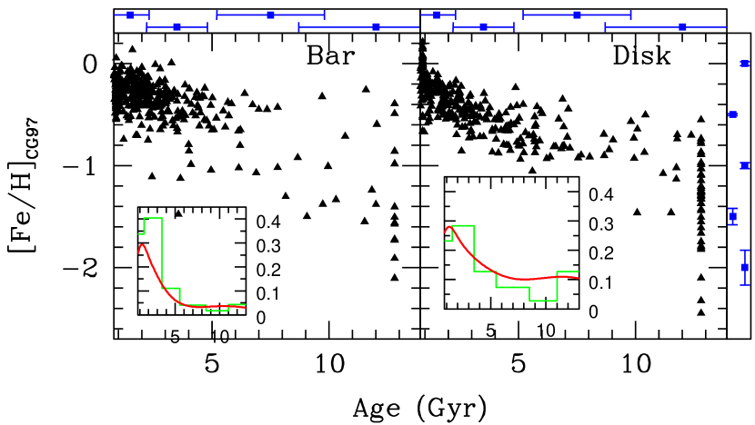
Figure 13: Same as Figure 11 but for the bar (left) and the disk fields combined (right).

Now we will compare the global AMR obtained for the disk with that observed in the bar. The bar stellar ages have been obtained using the relation calculated in Section 6. The age versus metallicity for each star in the bar (left) and disk (right) have been plotted in Figure 13. Notice that with a different method and different stellar evolution models, the AMR obtained here for the bar is quite similar to that obtained by Cole et al. (2005). We performed a $\chi^{2}$ test as before between the galaxy disk and bar AMRs. They are the same to within a probability of 90 per cent. However, a visual comparison would indicate that, while in the disk the metallicity has risen monotonically over the last few Gyr, this is not the case for the bar. However, from the comparison of the mean metallicities and the errorbars for stars in this youngest bin (1–3 Gyr) it appears that this difference is statistically significant.

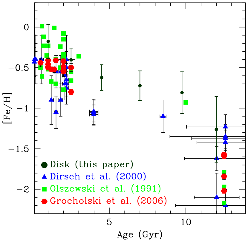
Figure 14: LMC clusters AMR by Olszewski et al. (1991, squares); Dirsch et al. (2000, triangles) and Grocholski et al. (2006, hexagons). The mean metallicity in six age bins of our global disk has been plotted (filled points). Note that the metallicity scales of each work may not be exactly the same.

The global disk AMR is qualitatively similar to that of the LMC cluster system (e.g. Olszewski et al., 1991; Dirsch et al., 2000), except for the lack of intermediate-age clusters (Figure 14). Clusters show a rapid enrichment phase around 10 Gyr ago which is also observed in the disk and the bar. The second period of chemical enrichment in the last 3 Gyr is also observed both in the field and in the clusters. The field intermediate-age stars may have contributed to the chemical enrichment at recent times. Note that the Grocholski et al. (2006) sample has a maximum metallicity [Fe/H]=-0.6, i.e. it does not seem to participate on the high metallicity tail at young ages that we and the other authors analysing clusters samples find. In the three works, there are a number of young clusters with low metallicity for their age, which Bekki & Chiba (2007) associate with metal-poor gas stripped from the SMC due to tidal interaction between the SMC, LMC and the Galaxy over the last 2 Gyr. A few stars also have low metallicity for their age in our sample, but they represent a minor contribution to the total.

7.4 The Star Formation History

More information can be retrieved from the AMRs. In particular we can also derive an approximate SFH of the LMC if we can establish that the observed stars are representative of the total population. The number of stars in each age bin can be transformed into stellar total mass, after accounting for the number of stars with a given age that have already died. To evaluate this correction we have computed a synthetic CMD using IAC-star (Aparicio & Gallart, 2004). We have assumed a constant SFR and used the relations derived for the chemical enrichment. As we have only observed a fraction of the total stars in the region of the RGB, we have rescaled the result to the total number of stars in this region.

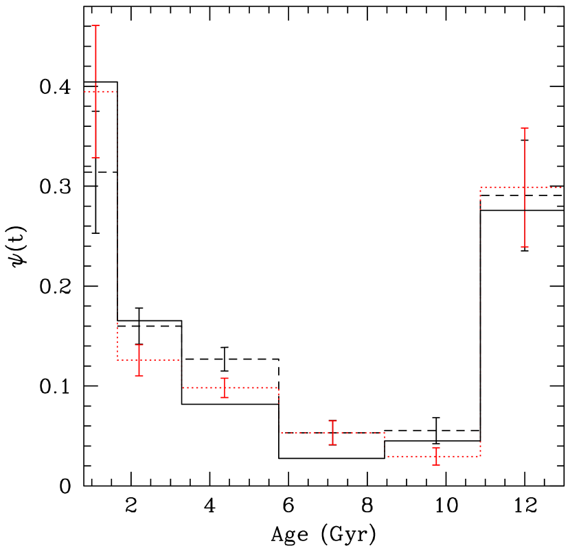
Figure 15: Results of the test on the reliability of the SFH computed using our spectroscopic RGB sample. Solid line: injected SFH; dashed line: mean and sigma of the recovered SFH after the Hydra filter assignment simulation; dotted line: the same as dashed one but with the age obtained from Equation 2. See text for detail.

In order to check whether the procedure used to select the stars observed spectroscopically introduces any bias in the computed SFH, we have calculated a synthetic CMD with a known chemical enrichment history and SFR. It was computed such that the number of stars in the selection region was the same as in the field at 3°. The input SFR as a function of age, $\psi(t)$, is plotted as a solid line in Figure 15. To check that the selection criteria did not introduce biases, we have selected objects from this synthetic CMD in the same way as from the LMC fields (see Figure 1). We assigned random positions to each synthetic star and, using the HYDRA configuration software, we computed 20 test configurations. The number of objects selected in each configuration, about 115, is similar to the observed stars in the LMC fields. For each test configuration, we calculated $\psi(t)$ following the procedure described above. The mean of the 20 total tests is the dashed line in Figure 15. The error bars are the standard deviation of the 20 tests. We repeated the same test, but obtaining the ages of each synthetic star using Equation 2. The result is the dotted line in Figure 15. As we can see in this Figure, the recovered $\psi(t)$ are consistent with the real one. In half of the bins the differences are within the error bars and in the rest they are within 3$\sigma$.

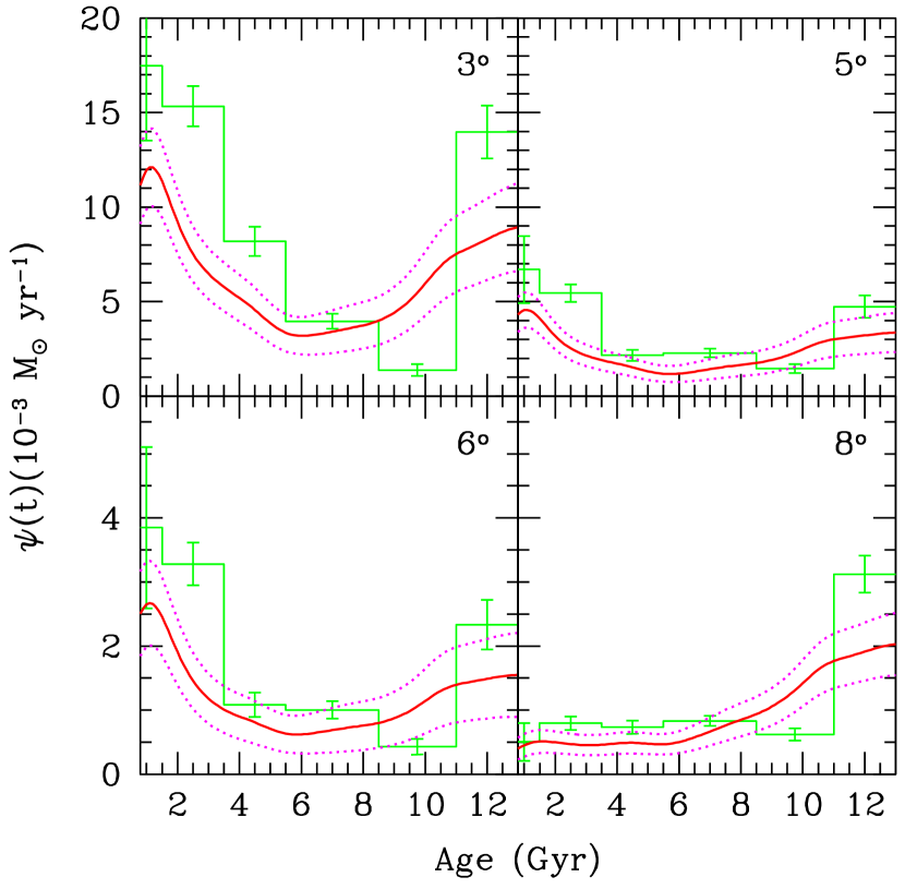
Figure 16: SFR, as a function of time, for our four fields. Note that the $y$-axis scale is different in the top and bottom panels. Histogram is the $\psi(t)$ computed from the age distribution without taking into account the age uncertainty. Solid line is the same but computed by taken into account the age error, while dotted lines are its uncertainty.

The $\psi(t)$ derived from our four fields are shown in Figure 16 (solid line), which has been computed from the age distribution, taking into account the age error (see Figure 7). The uncertainty in the computed $\psi(t)$ has been estimated as the square root of the SFR value for each age (dotted lines). However, values of the SFR for different ages are not independent from each other because the integral for the full age interval is a boundary condition of the solution. In other words, fluctuations above the best solution should be compensated by others below it, and a solution close to, for example, the upper (or the lower) dashed line is very unlike. As a comparison, the $\psi(t)$ computed without taking into account the age error has also been plotted in Figure 16. All fields have a first episode of star formation more than 10 Gyrs ago. Then, $\psi(t)$ decreases until $\sim$5 Gyr ago, when it rises again in the inner regions of the LMC (r$\leq$6°). This enhancement of $\psi(t)$ is not observed in the outermost field.

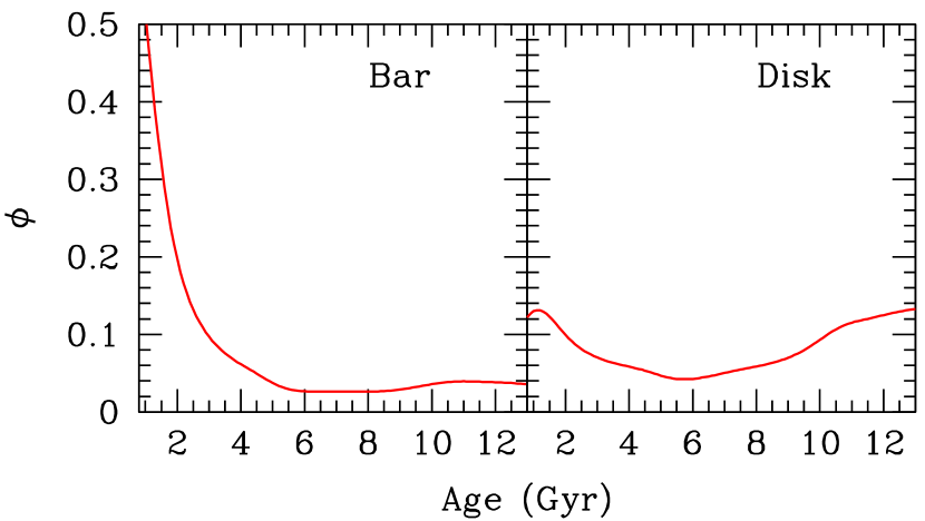
Figure 17: SFR as a function of time for the bar (left) and disk (right) derived from the spectroscopic sample.

We followed the same procedure to calculate $\psi(t)$ for the bar stars. The bar $\psi(t)$ is shown in Figure 17. In this case we do not know the total number of objects in the region where the observed stars were selected. For this reason, we have plotted the percentage, over the total, that the SFR represents in each age bin. In the right panel of the same Figure, the $\psi(t)$ of the disk, obtained as a combination of the four fields in our sample, is shown. The bar $\psi(t)$ is similar to that derived in small fields from HST deep photometry (Holtzman et al., 1999; Smecker-Hane et al., 2002), as indeed is expected since the HST fields are in the same region in which the RGB stars were observed. Both in the bar and in the disk, the galaxy started forming stars more than 10 Gyr ago, although in the bar the initial enhancement of $\psi(t)$ is not observed. For intermediate ages, the SFR was low until about 3 Gyr ago, when another increase in the SFR, which is particularly intense in the bar, is observed. This is consistent with previous investigations (e.g. Hardy et al., 1984; Smecker-Hane et al., 2002) and with the SFR derived from the clusters. The cluster age gap coincides with the age interval in which star formation has been less efficient.

7.5 A Chemical Evolution Model for the LMC

In what follows we use the AMR to obtain information on the physical parameters governing the chemical evolution of the LMC. As a first approximation, we will try to reproduce the derived relations with simple models.

Under the assumption of instantaneous recycling approximation, following Tinsley (1980) and Peimbert, Colin & Sarmiento (1994), the heavy-element mass fraction in the ISM, $Z$, evolves via:

$$\mu\frac{dZ}{d\mu}=\frac{y(1-R)\psi+(Z_{f}-Z)f_{I}}{-(1-R)\psi+(f_{I}-f_{O})(1-\mu)}$$ (3)

where $f_{I}$ and $f_{O}$ are the inflow and outflow rates respectively, $Z_{f}$ is the metallicity of the infall gas, $y$ denotes the yield, $R$ is the mass fraction returned to the interstellar medium by a generation of stars, relative to the mass locked in stars and stellar remnants in that generation, $\psi$ is the SFR and $\mu$ is defined as $\mu=M_{g}/M_{b}$, where M_g is the gas mass and M_b is the total baryonic mass, i.e., the mass participating in the chemical evolution process. In general, $Z,\mu,\psi,f_{I}$ and $f_{O}$ are explicit functions of time, while $R$ and $y$ may change according to characteristics of the stellar population like metallicity and initial mass function, but are usually assumed to be constant for a given population.

When there are no gas flows in and out of the system ($f_{I}=f_{O}=0$), the model is called a closed-box model and the solution to Equation 3 provides the variation of $Z(t)$ as a function of $\mu(t)$ via

$$Z(t)=Z_{i}+y\ln\mu(t)^{-1}$$ (4)

In an infall scenario, in which gas flows into the system at a rate proportional to the amount of star formation, $f_{I}=\alpha(1-R)\psi$, $\alpha$ being a free parameter, we can integrate Equation 3 for $\alpha\neq 1$, assuming that $f_{O}=0$, and obtaining:

$$Z(t)=Z_{i}+\frac{y+Z_{f}\alpha}{\alpha}\left[1-\left(\alpha-\frac{1-\alpha}{\mu(t)}\right)^{-\alpha/(1-\alpha)}\right]$$ (5)

For $\alpha$=1, the solution of Equation 3 is

$$Z=Z_{i}+y\left[1-e^{\left(1-\mu^{-1}\right)}\right]$$ (6)

In an outflow scenario, in which gas scapes from the system at a rate $f_{O}=\lambda(1-R)\psi$, $\lambda$ being a free parameter, we obtain from Equation 3 assuming $f_{I}=0$, and for ($\lambda\neq 1$):

$$Z(t)=Z_{i}+\frac{y}{\lambda-1}\ln\left[\frac{\lambda-1}{\mu(t)}-\lambda\right]$$ (7)

Finally, we will consider a model combination of inflow and outflow, and assume that the system gas flow is proportional to the mass that has taken part in the star formation: $f=(\alpha-\lambda)(1-R)\psi$, where we can define $\beta=\alpha-\lambda$. In this case, we can integrate Equation 3 for $\beta\neq$1, to obtain

$$Z(t)=Z_{i}+\frac{y+Z_{f}\alpha}{\alpha}\left[1-\left(\beta-\frac{1-\beta}{\mu(t)}\right)^{-\beta/(1-\beta)}\right]$$ (8)

In summary, the chemical evolution of the galaxy is given by the yield $y$, the initial metallicity of the gas Z_i, the fraction of gas mass $\mu(t)$, which is a function of $\psi(t)$, and $R$, the mass fraction returned to the interstellar medium. In the case of inflow and/or outflow, also by the additional parameters $\alpha$ and $\lambda$.

We can now apply the former relations to the LMC. In the previous section we have derived $\psi(t)$ for the LMC bar and disk, the latter being obtained from the combination of the four fields in our sample. $\mu$ is computed explicitly as a function of time from $\psi(t)$, the balance of gas flowing to and from the system, and using as a boundary condition the current LMC gas fraction. In the case of the LMC disk, we have assumed the value derived by Kim et al. (1998) from observations of H I. These authors derived $M_{g}=5.2\times 10^{8}M_{\odot}$ and estimated that the total mass of the disk is $M_{b}=2.5\times 10^{9}M_{\odot}$. With these values, we find the current gas fraction in the disk, $\mu_{f}=0.21$. For the bar we have assumed the value of $\mu=0.08$ given by Westerlund et al. (1990). For the yield, we have assumed the value obtained by Pagel & Tautvaisiene (1995) for the solar neighborhood, $y=0.014$. Assuming the Scalo (1986) initial mass function, Maeder (1993) calculated a returned fraction associated to this yield of $R=0.44$. Putting all these ingredients together, we will now explore several scenarios in order to reproduce the AMR of the disk and the bar.

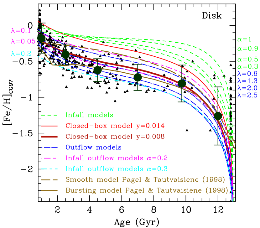
Figure 18: Chemical evolution models overplotted on the AMR for the disk. Red solid lines are the closed-box models with $y=0.008$, (thick line) and $y=0.014$ (thin line), respectively. Blue dot-dashed lines are outflow models for $\lambda=$ 0.6, 1.3, 2.0 and 2.5. Green dashed lines are infall models with $\alpha=$ 1, 0.9, 0.5 and 0.3. Pink long–short dashed lines are models with infall and outflow for $\alpha=$ 0.2, and $\lambda=$ 0.1 (upper) and 0.05 (lower). Finally, cyan short-long dashed line is a model with inflow and outflow for $\alpha=$ 0.3 and $\lambda=$ 0.2. All infall and outflow models assume $y=0.014$. The brown solid and dashed lines represent the bursting and smooth models computed by Pagel & Tautvaisiene (1998).

In Figure 18 we have plotted the age and metallicity of each star in the disk, together with the mean metallicity and its dispersion, for stars in each age bin. In this figure, chemical evolution models have been superposed for different scenarios and parameter assumptions (see the figure caption). In the case of the infall models (green dashed lines), we have assumed a zero-metallicity infalling gas, in order to obtain the current metallicity. They do not reproduce the general behavior of the observed AMR. The disk AMR is well reproduced by outflow models (blue dot-dashed lines) with a relatively large range of $\lambda$. Finally, the combination of inflow and outflow (pink and cyan long–short dashed lines) models also reproduce the metallicity tendency (in this case the model that best matches the observed data has $\alpha$ = 0.2 and $\lambda$ = 0.05). The previous models have been computed assuming the yield observed in the solar neighborhood which is probably too large for the LMC. With a smaller yield, $y=0.008$ (red thick solid line), the observed AMR can be reproduced by a closed-box model. This yield would correspond to stars with $Z=0.001$ (see Maeder, 1993, for details), which is slightly low compared with the mean LMC metallicity. Bursting and smooth models computed by Pagel & Tautvaisiene (1998) have been plotted as comparison (brown lines). The bursting model was computed assuming two burst of star formation, one about 12 Gyr ago and a strong one about 3 Gyr ago, and some fraction of infall and outflow. Note that their predicted values agree with our mean metallicity for each age bin, within the errorbars, specially at old and intermediate–age. It also qualitatively agrees with the episode of faster chemical evolution with started around $\sim$2 Gyr ago. The smooth model was computed assuming a constant star formation rate and does not match with the observations.

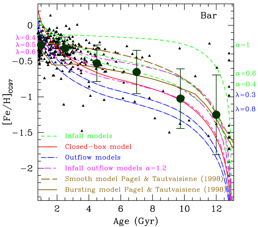
Figure 19: As Figure 18 for the bar. Red solid line is a closed-box model. Blue dot-dashed lines are outflow models for $\lambda=$ 0.8 and 0.3. Green short-dashed lines are infall models with $\alpha=$ 1, 0.6 and 0.4. Pink long–short dashed lines are models with inflow and outflow for $\alpha=$ 1.2 and $\lambda=$ 0.4, 0.5 and 0.6. All models assume y=0.014. As in the previous figure, brown lines represent the models computed by Pagel & Tautvaisiene (1998).

In the case of the bar (Figure 19), the very slowly rising metallicity, almost constant over the last few Gyr, is best reproduced by the combination of models with inflow and outflow with infall parameter $\alpha$ = 1.2 and $\lambda$ = 0.4-0.6 (pink long–short dashed lines). Infall models (green dashed lines) with $\alpha$ = 0.4-0.6 marginally reproduce the observed trend, but they predict higher metallicities than observed in the last few Gyr, unless a smaller yield would be assumed. Finally, outflow and closed-box models predict a rise of metallicity in the last few Gyr more steep than observed. The Pagel & Tautvaisiene (1998) bursting model agrees worse with the bar AMR than with that of the disk, specially in the youngest age bins.

8 Conclusions

Using infrared spectra in the CaT region, we have obtained metallicities and radial velocities for a sample of stars in four LMC fields. Metallicities have been calculated using the relationships between the equivalent width of the CaT lines, $\Sigma Ca$, and metallicity derived in Paper II. In addition, we have estimated the age of each star using a relationship derived from a synthetic CMD which, from the color, magnitude and metallicity of a star, allow us to estimate its age. The main results of this paper are:

• The velocity distribution observed in each field agrees with the rotational thick disk kinematics of the LMC. The velocity dispersion is slightly larger for the most metal-poor stars. However, the values obtained do not indicate the presence of a kinematically hot halo.

• The metallicity distribution of each field has a well defined peak with a tail toward low metallicities. The mean metallicity is constant until the field at 6° ([Fe/H]$\sim$-0.5 dex), and is a factor two more metal-poor for the outermost field ([Fe/H]$\sim$-0.8 dex).

• The AMR observed in each disk field is compatible with a single global relationship for the disk. We conclude that the outermost field is more metal-poor on average because it contains a lower fraction of relatively young stars (age$\leq$5 Gyr), which are also more metal-rich.

• The disk AMR shows a prompt initial chemical enrichment. Subsequently, the metallicity increased very slowly until about 3 Gyr ago, when the rate of metal enrichment increased again. This AMR is similar to that of the cluster system, except for the lack of clusters with ages between 3 and 10 Gyr. The recent fast enrichment observed in the disk and in the cluster system is not observed in the bar.

• The $\psi(t)$ of the three innermost fields show a first episode of star formation until about 10 Gyr ago, followed by a period with a low SFR until $\sim$5 Gyr ago, when the SFR increases, and reaches its highest values $\sim$2-3 Gyr ago. The outermost field does not show the recent increase of SFR. The second main episode is also observed, and is more prominent in the bar, where an increased SFR at old ages is not observed. The lower SFR between 5 and 10 Gyr ago is probably related to the age-gap observed in the clusters.

• Under the assumption of a solar yield, the disk AMR is well reproduced either by a chemical evolution model with outflow with $\lambda$ between 1 and 2, so the disk losses the same amount of gas that has taken part in the star formation, or by models combining infall and outflow with $\alpha$=0.2 and $\lambda$=0.05, which means that the galaxy is almost a closed-box system. With a smaller yield, the AMR could also be reproduced with a closed-box model. The bar AMR is well reproduced by models with a combination of inflow and outflow with $\alpha$=1.2 and $\lambda$ between 0.4 and 0.5. This suggests that the amount of infalling gas was larger than the amount that participated in the star formation in the bar, and also that the amount of gas that escaped the bar was 50% of the total that participated in star formation.

9 Discussion

The main result in this paper is that all our fields, covering galactocentric radius from 3° to 8° from the center (2.7 to 7.2 kpc) share a very similar AMR. The mean metallicity is very similar in the three innermost fields ([Fe/H] $\simeq$-0.5 dex), and it is a factor of $\simeq 2$ smaller in the outermost field ([Fe/H] $\simeq$-0.8 dex). Because the AMRs are the same, this has to be related with the lower fraction of relatively young stars (age $\leq$ 5 Gyr), which are also more metal-rich, in the outer part. We find, therefore, a change in the age composition of the disk population beyond a certain radius ($\simeq$ 6 kpc; note however that in this study we are only sensitive to populations older than $\simeq$ 0.8 Gyr, and that differences among fields for younger ages could also exist), while the chemical enrichment history seems to be shared by all fields.

The comparison of the AMR observed in the disk with simple chemical evolution models suggests that the LMC is most likely losing some of its gas. This is in agreement with the work by Nidever et al. (2007) which suggests that the main contribution to the Magellanic Stream comes from the LMC instead of from the SMC as it was believed until now (e.g. Putman et al., 2003). Alternatively, the LMC could be an almost closed-box system with small gas exchanges ($\alpha$=0.2, $\lambda$=0.05). This could be in agreement with the models by Bekki & Chiba (2007) which suggest that the LMC has received metal-poor gas from the SMC in the last 2 Gyr. In our field we observed some stars with a low metallicity to which we assign an age younger than 2 Gyr. However, the uncertainty in the age determination is large.

We have also obtained the AMR of the LMC bar from the data by Cole et al. (2005). The bar AMR differs from the one of the disk in the last 5 Gyr: while in the disk the metallicity has increased in this time, in the bar it has remained approximately constant. This feature is best reproduced by models combination of outflow and a relatively large infall of pristine gas. Models with a smaller yield, but with an infall of previously enriched gas also reproduce the observed bar AMR. This would be in agreement with the prediction that a typical bar instability pushes the gas of the disk towards the center (Sellwood & Wilkinson, 1993), so the infall gas is expected to be previously pre-enrichment by the disk chemical evolution. This would be also the case in the scenario suggested by Bekki & Chiba (2005), in which the bar would have formed from disk material as a consequence of tidal interactions between the LMC, the SMC and the Milky Way about 5 Gyr ago, the moment when the bar AMR differs from that of the disk. Also, a bar is expected to destroy any metallicity gradient within a certain radius, as it is observed.

Gallart et al. (2004) derived the LMC surface brightness profile using deep resolved star photometry of the four fields in the current spectroscopic study, and found that it remains exponential to a radius of 8° ($\simeq$ 7 kpc), with no evidence of disk truncation. Combining this information with that on the deep CMD of the outermost field, which contains a large fraction of intermediate-age stars, they concluded that the LMC disk extends (and dominates over a possible halo) at a distance of at least 7 kpc from its center. In the present study, the kinematics of the stars in these four fields confirm this conclusion: the velocity dispersion of all four fields is similar, around 20 km/sec. If the stars are binned by metallicity, the velocity dispersion of the most metal-poor bin is slightly larger than that of the metal-richer bins ($\sigma_{V}\simeq 25$ km/sec as opposed to $\simeq 20$ km/sec) but still not large enough to indicate the presence of a halo, even one formed as a consequence of the interaction with the Galaxy. In this case, Bekki et al. (2004) predicted a velocity dispersion $\simeq$ 40 km/s at a distance of 7.5 kpc from the LMC center (similar to the distance of our outermost field). Other authors have also failed to find a kinematically hot halo (Freeman, Illingworth, & Oemler, 1983; Schommer et al., 1992; Graff et al., 2000; Zhao et al., 2003). The first evidence of the presence of a kinetically hot, old spheroidal population was reported by Hughes, Wood, & Reid (1991) using a sample of long period variables, which are related to an old stellar population. Recently, Minniti et al. (2003) observed spectroscopically a sample of 43 bar RR Lyrae stars, and obtained a large velocity dispersion (53 $\pm$ 10 km s^-1) for them. It is possible that our failure (and that of other authors) to find evidence of a hot stellar halo is related with a low contrast of the halo population with respect to the disk one, even at large galactocentric radius as our outermost field.

Figure 2: Example of sky subtraction. Top: raw spectrum. Middle: sky spectrum obtained from a combination of fibers located on the sky. Bottom: The final spectrum after sky subtraction.

Figure 8: Ages derived for the cluster sample in Paper II, using Equation 2 and BaSTI and Padova models versus the reference ages. The solid lines are the one-to-one relation.

Figure 10: Radial velocity dispersion of the disk stars as a function of metallicity. Although the velocity dispersion increases from metal-rich to metal-poor stars, this increment is not clear enough to conclude that a metal-poor stellar halo is present.

Table 1: LMC RGB stars observed

$\alpha_{2000}$	$\delta_{2000}$	$\Sigma$ Ca	$\sigma_{\Sigma Ca}$	V	I	$V_{r}(kms^{-1}$)	$\sigma_{V_{r}}(kms^{-1}$)	Comments
05:08:53.92	-66:49:55.1	7.8	0.8	17.67	16.36	287.3	0.7
05:08:55.21	-66:47:34.7	8.7	0.2	16.66	14.70	240.9	0.6
05:08:53.89	-67:02:50.0	2.4	0.2	17.19	14.25	23.0	0.6	No member
05:08:55.40	-66:53:45.4	8.9	0.4	16.79	15.09	292.3	0.5
05:08:58.58	-66:45:49.2	9.4	0.2	16.00	13.99	291.9	0.5

Note. — Table 1 is published in its entirety in the electronic edition of The Astronomical Journal. A portion is shown here for guidance regarding its form and content

Table 2: Radial velocities and velocity dispersion for each field.

Field	$\langle V_{r}\rangle(kms^{-1})$	$\sigma_{V}(kms^{-1})$
Bar	260	24
3°	269	27
5°	278	20
6°	293	15
8°	282	14

Table 3: Line and continuum bandpasses

Line Bandpasses (Å)	Continuum bandpasses (Å)
8484-8513	8474-8484
8522-8562	8563-8577
8642-8682	8619-8642
$\cdots$	8799-8725
$\cdots$	8776-8792

Table 4: Coefficients of Equation 2.

Model	a	b	c	d	f	g	h	$\sigma$
BaSTI	2.57$\pm$0.10	9.72$\pm$0.15	0.70$\pm$0.003	-1.51$\pm$0.007	-3.86$\pm$0.08	-0.19$\pm$0.007	0.49$\pm$0.01	0.38
Padova	1.69$\pm$0.07	10.6$\pm$0.1	0.75$\pm$0.002	-1.87$\pm$0.007	-4.14$\pm$0.06	-0.24$\pm$0.006	0.51$\pm$0.009	0.37

Table 5: Velocity dispersion for each metallicity bin.

[Fe/H]	Age (Gyr)	N∗	$\langle V_{r}\rangle(kms^{-1})$	$\sigma_{V}(kms^{-1})$
$\geq$-0.5	$<$3	226	0.1	20.5
-0.5 to -1	2-10	178	1.9	20.5
$\leq$-1	$>$10	100	1.8	26.4

Table 6: Mean values of metallicity distributions.

Field	$\langle$[Fe/H]$\rangle$	$\sigma_{[Fe/H]}$
Bar	-0.39	0.19
3°	-0.47	0.31
5°	-0.50	0.37
6°	-0.45	0.31
8°	-0.79	0.44

Table 7: Average metallicity in six age bins.

Field	$\langle[Fe/H]_{\leq 1.5}\rangle$	$\langle[Fe/H]_{1.5-3.5}\rangle$	$\langle[Fe/H]_{3.5-5.5}\rangle$	$\langle[Fe/H]_{5.5-8.5}\rangle$	$\langle[Fe/H]_{8.5-11}\rangle$	$\langle[Fe/H]_{\geq 11}\rangle$	$\chi^{2}_{\nu}$
Bar	-0.27$\pm$0.13	-0.32$\pm$0.16	-0.53$\pm$0.26	-0.65$\pm$0.30	-1.02$\pm$0.41	-1.25$\pm$0.56	…
Disk	-0.17$\pm$0.21	-0.39$\pm$0.15	-0.60$\pm$0.16	-0.71$\pm$0.18	-0.80$\pm$0.27	-1.25$\pm$0.41	…
3°	-0.16$\pm$0.17	-0.40$\pm$0.14	-0.58$\pm$0.15	-0.67$\pm$0.20	-0.69$\pm$0.07	-1.13$\pm$0.43	0.05
5°	-0.16$\pm$0.28	-0.39$\pm$0.15	-0.63$\pm$0.18	-0.72$\pm$0.16	-0.83$\pm$0.35	-1.39$\pm$0.42	0.02
6°	-0.15$\pm$0.16	-0.38$\pm$0.16	-0.60$\pm$0.16	-0.75$\pm$0.20	-0.83$\pm$0.14	-1.34$\pm$0.24	0.02
8°	-0.16$\pm$0.21	-0.45$\pm$0.13	-0.62$\pm$0.20	-0.89$\pm$0.16	-0.92$\pm$0.18	-1.25$\pm$0.32	0.16

References

- Alves (2004) Alves, D. R. 2004, New A Rev., 49, astro-ph0408336
- Aparicio & Gallart (2004) Aparicio, A., & Gallart, C. 2004, A&A, 128, 1465
- Bekki et al. (2004) Bekki, K., Couch, W. J., Beasley, M. A., Forbes, M. A., Chiba, M., & Da Costa, G. S. 2004, ApJ, 610, L93
- Bekki & Chiba (2005) Bekki, K., & Chiba, M., 2005, MNRAS, 356, 680
- Bekki & Chiba (2007) Bekki, K., & Chiba, M., 2007, MNRAS, in press
- Bertelli et al. (1992) Bertelli, G., Mateo, M., Chiosi, C. & Bressan, A. 1992, ApJ, 388, 400
- Bica et al. (1998) Bica, E., Geisler, D., Dottori, H., Clariá, J. J., Piatti, A. E., & Santos, J. F. C., Jr. 1998, AJ, 116, 723
- Carrera et al. (2007) Carrera, R., Gallart, C., Pancino, E. & Zinn, R. 2007, AJ, 134, 1298 (Paper II)
- Carretta & Gratton (1997) Carretta, E., & Gratton, R. G. 1997, A&AS, 121, 95 (CG97)
- Castro et al. (2001) Castro, R., Santiago, B. X., Gilmore, G. F., Beaulieu, S. & Johnson, R. A. 2001, MNRAS, 326, 333
- Cenarro et al. (2001) Cenarro, A. J., Cardiel, N., Gorgas, J., Peletier, R. F., Vazdekis, A., & Prada, F. 2001, MNRAS, 326, 959
- Cioni & Habing (2003) Cioni, M.-R. L., & Habing, H. J. 2003, A&A, 402, 133
- Cole, Smecker-Hane, & Gallagher (2000) Cole, A. A., Smecker-Hane, T. A., & Gallagher III, J. S. 2000, AJ, 120, 1808
- Cole et al. (2005) Cole, A. A., Tolstoy, E., Gallagher III, J. S. & Smecker-Hane, T. A. 2005, AJ, 129, 1465
- Dirsch et al. (2000) Dirsch, B., Richtler, T., Gieren, W.P. & Hilker, M. 2000, A&A, 360, 133
- Dopita et al. (1997) Dopita M. A., Vassiliadis, E., Wood, P.R., Meatheringhan, J. S., Harrington, J. P., Bohlin, R. C., Ford, H.C., Stecher, T. P., & Maran, S. P. 1997, ApJ, 474, 188
- Freeman, Illingworth, & Oemler (1983) Freeman, K. C., Illingworth, G., & Oemler Jr, A. 1983, ApJ, 272, 488
- Gallart et al. (2004) Gallart, C., Stetson, P. B., Hardy, E., Pont, F., & Zinn, R. 2004, ApJ, 614, L109
- Gallart, Zoccali & Aparicio (2005) Gallart, C., Zoccali, M., & Aparicio, A. 2005, ARA&A, 43, 387
- Gallart et al. (2007) Gallart, C., Stetson, P. B., Pont, F., Hardy, E., & Zinn, R. 2007, in preparation, (Paper I)
- Geisler et al. (1995) Geisler, D., Piatti, A. E., Clariá, J. J., & Minniti, D. 1995, AJ, 109, 605
- Geisler et al. (1997) Geisler, D., Bica, E., Dottori, H., Clariá, J. J., Piatti, A. E., & Santos Jr., J. F. C. 1997, AJ, 114, 1920
- Girardi et al. (2002) Girardi, L., Bertelli, G., Bressan. A., Chiosi, C., Groenewegen, M: A. T., Marigo, P., Salasnich, B., & Weiss, A. 2002, A&A, 391, 195
- Gratton et al. (2004) Gratton, R. G., Bragaglia, A., Clementini, G., Carretta, E., Di Fabrizio, L., Maio, M., & Taribello, E. 2004, A&A, 421, 937
- Graff et al. (2000) Graff, D. S., Gould, A. P., Suntzeff, N. B., Schommer, R. A., & Hardy, E. 2000, ApJ, 540, 211
- Grocholski et al. (2006) Grocholski, A. J., Cole, A. A., Sarajedini, A., Geisler, D., & Smith, V. V. 2006, AJ, 132, 1630
- Hardy et al. (1984) Hardy, E., Buonanno, R., Corsi, C. E., Janes, K. A. & Schommer, R. A. 1984, ApJ, 278, 592
- Hill, Andrievsky, & Spite (1995) Hill, V., Andrievsky, S., & Spite, M. 1995, A&A, 293, 347
- Holtzman et al. (1999) Holtzman, J. A., Gallagher, J. S., III, Cole, A. A., Mould, J. R., Grillmair, C. J., Ballester, G. E., Burrows, C. J., Clarke, J. T., Crisp, D., Evans, R. W., Griffiths, R. E., Hester, J. J., Hoessel, J. G., Scowen, P. A., Stapelfeldt, K. R., Trauger, J. T. & Watson, A. M., 1999, AJ, 118, 2262
- Hughes, Wood, & Reid (1991) Hughes, S. M. G., Wood, P. R., & Reid, N. 1991, AJ, 101, 1304
- Kim et al. (1998) Kim, S., Staveley-Smith, L., Dopita, M. A., Freeman, K. C., Sault, R. J., Kesteven, M. J. & McConnell, D. 1998, ApJ, 503, 674
- Koch et al. (2006) Koch, A., Grebel, E. K., Wyse, R. F. G., Kleyna, J. T., Wilkinson, M. I., Harbeck, D. R., Gilmore, G. F., & Evans, N. W.. 2006, AJ, 131, 895
- Kontizas, Kontizas, & Michalitsiano (1993) Kontizas, M., Kontizas, E., & Michalitsiano, A. G. 1993, A&A, 269, 107
- Kraft & Ivans (2003) Kraft, R. P., & Ivans, I. I. 2003, PASP, 115, 143
- Kunkel et al. (1997) Kunkel, W. E., Demers, S., Irwin, M. J., & Albert, L. 1997, ApJ, 488, L129
- Maeder (1993) Maeder, A. 1993, A&A, 268, 833
- Minniti et al. (2003) Minniti, D., Borissova, J., Rejkuba, M., Alves, D. R., Cook, K. H. & Freeman, K. C., 2003, Science, 301, 5639
- Nidever et al. (2007) Nidever, D. L., Majewski, S. R. & Butler Burton, W. 2007, ApJ, submitted
- Olszewski et al. (1991) Olszewski, E. W., Schommer, R. A., Suntzeff, N. B., & Harris, H., C. 1991, AJ, 101, 515
- Olszewski et al. (1996) Olszewski, E. W., Suntzeff, N. B., & Mateo, M. 1996, ARA&A, 34, 511
- Pagel & Tautvaisiene (1995) Pagel, B. E. J., & Tautvaisiene, G. 1995, MNRAS, 276, 505
- Pagel & Tautvaisiene (1998) Pagel, B. E. J., & Tautvaisiene, G. 1998, MNRAS, 299, 535
- Peimbert, Colin & Sarmiento (1994) Peimbert, M., Colin, P. & Sarmiento, A. 1994, in ”Violent Star Formation From 20 Doradus to QSOs” ed. G. Tenorio-Tagle. Cambridge University Press.
- Pietrinferni et al. (2004) Pietrinferni, A., Cassisi, S., Salaris, M., & Castelli, F. 2004, ApJ, 612, 168
- Pont et al. (2004) Pont, F., Zinn, R., Gallart, C., Hardy, E., & Winnick, R. 2004, AJ, 127, 840
- Putman et al. (2003) Putman, M. E., Staveley-Smith, L., Freeman K. C., Gibson, B. K. & Barnes, D. G. 2003, ApJ, 586, 170
- Salaris & Weiss (2002) Salaris, M., & Weiss, A. 2002, A&A, 388, 492
- Salaris, Weiss, & Percival (2004) Salaris, M., Weiss, A., & Percival, S. M. 2004, A&A, 414, 163
- Santos Jr. et al. (1999) Santos Jr., F. F. C., Piatti, A. E., Cariá, J. J., Geisler, D., & Dottori, H. 1999, AJ, 117, 2841
- Scalo (1986) Scalo, J. M. 1986, Fund. Cosmic Phys., 11, 1
- Schommer et al. (1992) Schommer, R. A., Suntzeff, N. B., Olszewski, E. W. & Harris, H. C. 1992, AJ, 103, 447
- Sellwood & Wilkinson (1993) Sellwood, J. A. & Wilkinson, A. 1993, Reports on Progress in Physics, 56, 173
- Smecker-Hane et al. (2002) Smecker-Hane, T. A., Cole, A. A., Gallagher, J. S., III & Stetson, P. B. 2002, ApJ, 566, 239
- Spergel et al. (2003) Spergel, D. N., Verde, L., Peiris, H. V., Komatsu, E., Nolta, M. R., Bennett, C. L., Halpern, M., Hinshaw, G., Jarosik, N., Kogut, A., Limon, M., Meyer, S. S., Page, L., Tucker, G. S., Weiland, J. L., Wollack, E., Wright, E. L. 2003, ApJS, 148, 175
- Tinsley (1980) Tinsley, B. M., 1980, Fund. Cosmic Phys., 5, 287
- Tonry & Davis (1979) Tonry, J., & Davis, M. 1979, AJ, 84, 1511
- van Dokkun (2001) van Dokkun, P. G. 2001, PASP, 113, 1420
- Vallenari et al. (1996) Vallenari, A., Chiosi, C., Bertelli, G. & Ortolani, S. 1996, A&A, 309, 358
- Westerlund et al. (1990) Westerlund, B. E. 1990, A&A Rev., 2, 29
- Westerlund, Linde, & Lynga (1995) Westerlund, B. E., Linde, P. & Lynga, G. 1995, A&A, 298, 39
- Zinn & West (1984) Zinn, R., & West, M. J. 1984 ApJS, 55, 45
- Zhao et al. (2003) Zhao, H. S., Ibata, R., Lewis, G. F., & Irwin, M. J. 2003 MNRAS, 339, 701