Reducing the Spectral Index in
F-Term Hybrid Inflation

Abstract

We consider a class of well motivated supersymmetric models of F-term hybrid inflation (FHI) which can be linked to the supersymmetric grand unification. The predicted scalar spectral index $n_{\rm s}$ cannot be smaller than $0.97$ and can exceed unity including corrections from minimal supergravity, if the number of e-foldings corresponding to the pivot scale $k_{*}=0.002/{\rm Mpc}$ is around 50. These results are marginally consistent with the fitting of the three-year Wilkinson microwave anisotropy probe data by the standard power-law cosmological model with cold dark matter and a cosmological constant. However, $n_{\rm s}$ can be reduced by applying two mechanisms: (i) The utilization of a quasi-canonical Kähler potential with a convenient choice of a sign and (ii) the restriction of the number of e-foldings that $k_{*}$ suffered during FHI. In the case (i), we investigate the possible reduction of $n_{\rm s}$ without generating maxima and minima of the potential on the inflationary path. In the case (ii), the additional e-foldings required for solving the horizon and flatness problems can be generated by a subsequent stage of fast-roll [slow-roll] modular inflation realized by a string modulus which does [does not] acquire effective mass before the onset of modular inflation.

1 Introduction

A plethora of precise cosmological observations on the cosmic microwave background radiation (CMB) and the large-scale structure in the universe has strongly favored the idea of inflation [2] (for reviews see e.g. Refs. [3, 4, 5]). We focus on a set of well-motivated, popular and quite natural models [6] of supersymmetric (SUSY) F-term hybrid inflation (FHI) [7], realized [8] at (or very close to) the SUSY grand unified theory (GUT) scale $M_{\rm GUT}=2.86\times 10^{16}~{}{\rm GeV}$. Namely, we consider the standard [8], shifted [9] and smooth [10] FHI. In the context of global SUSY (and under the assumption that the problems of the standard big bag cosmology (SBB) are resolved exclusively by FHI), these models predict scalar spectral index, $n_{\rm s}$, extremely close to unity and without much running, $a_{\rm s}$. Moreover, corrections induced by minimal supergravity (mSUGRA) drive [11] $n_{\rm s}$ closer to unity or even upper than it.

These predictions are marginally consistent with the fitting of the three-year Wilkinson microwave anisotropy probe (WMAP3) results by the standard power-law cosmological model with cold dark matter and a cosmological constant ($\Lambda$CDM). Indeed, one obtains [12] that, at the pivot scale $k_{*}=0.002/{\rm Mpc}$, $n_{\rm s}$ is to satisfy the following rather narrow range of values:

$$n_{\rm s}=0.958\pm 0.016~{}\Rightarrow~{}0.926\lesssim n_{\rm s}\lesssim 0.99$$ (1)

at 95$\%$ confidence level with negligible $a_{\rm s}$.

A possible resolution of the tension between FHI and the data is suggested in Ref. [13]. There, it is argued that values of $n_{\rm s}$ between 0.98 and 1 can be made to be compatible with the data by taking into account a sub-dominant contribution to the curvature perturbation in the universe due to cosmic strings which may be (but are not necessarily [14]) formed during the phase transition at the end of FHI. However, in such a case, the GUT scale is constrained to values well below $M_{\rm GUT}$ [15, 16, 17]. In the following, we reconsider two other resolutions of the problem above without the existence of cosmic strings:

• FHI within quasi-canonical SUGRA (qSUGRA). In this scenario, we invoke [17, 18] a departure from mSUGRA, utilizing a quasi-canonical (we use the term coined originally in Ref. [19]) Kähler potential with a convenient arrangement of the sign of the next-to-minimal term. This yields a negative mass term for the inflaton in the inflationary potential which can lead to acceptable $n_{\rm s}$’s. In a sizable portion of the region in Eq. (1) a local minimum and maximum appear in the inflationary trajectory, thereby jeopardizing the attainment of FHI. In that case, we are obliged to assume suitable initial conditions, so that hilltop inflation [20] takes place as the inflaton rolls from the maximum down to smaller values. Therefore, $n_{\rm s}$ can become consistent with Eq. (1) but only at the cost of a mild tuning [17] of the initial conditions. On the other hand, we can show [21, 22] that acceptable $n_{\rm s}$’s can be obtained even without this minimum-maximum problem.

• FHI followed by modular inflation (MI). It is recently proposed [23] that a two-step inflationary set-up can allow acceptable $n_{\rm s}$’s in the context of FHI models even with canonical Kähler potential. The idea is to constrain the number of e-foldings that $k_{*}$ suffers during FHI to relatively small values, which reduces $n_{\rm s}$ to acceptable values. The additional number of e-foldings required for solving the horizon and flatness problems of SBB can be obtained by a second stage of inflation (named [23] complementary inflation) implemented at a lower scale. We can show that MI [24] (for another possibility see Ref. [25]), realized by a string modulus, can play successfully the role of complementary inflation. A key issue of this set-up is the evolution of the modulus before the onset of MI [26, 27]. We single out two cases according to whether or not the modulus acquires effective mass before the commencement of MI. We show that, in the first case, MI is of the slow-roll type and a very mild tuning of the initial value of the modulus is needed in order to obtain solution compatible with a number of constraints. In the second case, the initial value of the modulus can be predicted due to its evolution before MI, and MI turns out to be of the fast-roll [28] type. However, in our minimal set-up, an upper bound on the total number of e-foldings obtained during FHI emerges, which signalizes a new disturbing tuning. Possible ways out of this situation are also proposed.

In this presentation we reexamine the above ideas for the reduction of $n_{\rm s}$ within FHI, implementing the following improvements:

• In the case (i) we delineate the parametric space of the FHI models with acceptable $n_{\rm s}$’s maintaining the monotonicity of the inflationary potential and derive analytical expressions which approach fairly our numerical results.

• In the case (ii) we incorporate the nucleosynthesis (NS) constraint and we analyze the situation in which the inflaton of MI acquires mass before the onset of MI, under some simplified assumptions [29].

The text is organized as follows: In Sec. 2, we review the basic FHI models and in the following we present the two methods for the reduction of $n_{\rm s}$ using qSUGRA (Sec. 3) or constructing a two-step inflationary scenario (Sec. 4). Our conclusions are summarized in Sec. 5.

2 The FHI Models

We outline the salient features (the superpotential in Sec 2.1, the SUSY potential in Sec. 2.2 and the inflationary potential in Sec. 2.3) of the basic types of FHI and we present their predictions in Sec. 2.6, calculating a number of observable quantities introduced in Sec. 2.4, within the standard cosmological set-up described in Sec. 2.5.

2.1 The Relevant Superpotential

The F-term hybrid inflation can be realized [6] adopting one of the superpotentials below:

$$W=\left\{\matrix{\kappa S\left(\bar{\Phi}\Phi-M^{2}\right)\hfill&\mbox{for standard FHI},\hfill\cr\kappa S\left(\bar{\Phi}\Phi-M^{2}\right)-S{(\bar{\Phi}\Phi)^{2}\over M_{\rm S}^{2}}\hfill&\mbox{for shifted FHI},\hfill\cr S\left({(\bar{\Phi}\Phi)^{2}\over M_{\rm S}^{2}}-\mu_{\rm S}^{2}\right)\hfill&\mbox{for smooth FHI},\hfill\cr}\right.\mbox{where}$$ (2)

• $S$ is a left handed superfield, singlet under a GUT gauge group $G$,

• $\bar{\Phi}$, $\Phi$ is a pair of left handed superfields belonging to non-trivial conjugate representations of $G$, and reducing its rank by their vacuum expectation values (v.e.vs),

• $M_{\rm S}\sim 5\times 10^{17}~{}{\rm GeV}$ is an effective cutoff scale comparable with the string scale,

• $\kappa$ and $M,~{}\mu_{\rm S}~{}(\sim M_{\rm GUT})$ are parameters which can be made positive by field redefinitions.

The superpotential in Eq. (2) for standard FHI is the most general renormalizable superpotential consistent with a continuous R-symmetry [8] under which

$$S\ \rightarrow\ e^{i\alpha}\,S,~{}\bar{\Phi}\Phi\ \rightarrow\ \bar{\Phi}\Phi,~{}W\rightarrow\ e^{i\alpha}\,W.$$ (3)

Including in this superpotential the leading non-renormalizable term, one obtains the superpotential of shifted [9] FHI in Eq. (2). Finally, the superpotential of smooth [10] FHI can be produced if we impose an extra $Z_{2}$ symmetry under which $\Phi\rightarrow-\Phi$ and, therefore, only even powers of the combination $\bar{\Phi}\Phi$ can be allowed.

2.2 The SUSY Potential

The SUSY potential, $V_{\rm SUSY}$, extracted (see e.g. ref. [3]) from $W$ in Eq. (2) includes F and D-term contributions. Namely,

$$V_{\rm SUSY}=V_{\rm F}+V_{\rm D},~{}~{}\mbox{where}$$

• The F-term contribution can be written as:

  $$V_{\rm F}=\left\{\matrix{\kappa^{2}M^{4}\left(({\sf\Phi}^{2}-1)^{2}+2{\sf S}^{2}{\sf\Phi}^{2}\right)\hfill&\mbox{for standard FHI},\hfill\cr\kappa^{2}M^{4}\left(({\sf\Phi}^{2}-1-\xi{\sf\Phi}^{4})^{2}+2{\sf S}^{2}{\sf\Phi}^{2}(1-2\xi{\sf\Phi}^{2})^{2}\right)\hfill&\mbox{for shifted FHI},\hfill\cr\mu^{4}_{\rm S}\left((1-{\sf\Phi}^{4})^{2}+16{\sf S}^{2}{\sf\Phi}^{6}\right)\hfill&\mbox{for smooth FHI},\hfill\cr}\right.$$ (4)

  where the scalar components of the superfields are denoted by the same symbols as the corresponding superfields and

  $$\left\{\matrix{{\sf\Phi}=|\Phi|/M~{}~{}\mbox{and}~{}~{}{\sf S}=|S|/M\hfill&\mbox{for standard or shifted FHI,}\hfill\cr{\sf\Phi}=|\Phi|/2\sqrt{\mu_{\rm S}M_{\rm S}}~{}~{}\mbox{and}~{}~{}{\sf S}=|S|/\sqrt{2\mu_{\rm S}M_{\rm S}}\hfill&\mbox{for smooth FHI},\hfill\cr}\right.$$

  with $\xi=M^{2}/\kappa M_{\rm S}$ and $1/7.2<\xi<1/4$ [9].

  In Figs. 1, 2 and 3 we present the three dimensional plot of $V_{\rm F}$ versus $\pm{\sf\Phi}$ and ${\sf S}$ for standard, shifted and smooth FHI, respectively. The inflationary trajectories are also depicted by bold points, whereas the critical points by red/light points.

• The D-term contribution $V_{\rm D}$ vanishes for $|\bar{\Phi}|=|\Phi|$.

Using the derived $V_{\rm SUSY}$, we can understand that $W$ in Eq. (2) plays a twofold crucial role:

• It leads to the spontaneous breaking of $G$. Indeed, the vanishing of $V_{\rm F}$ gives the v.e.vs of the fields in the SUSY vacuum. Namely,

  $$\langle S\rangle=0~{}~{}\mbox{and}~{}~{}|\langle\bar{\Phi}\rangle|=|\langle\Phi\rangle|=v_{{}_{G}}=\left\{\matrix{M\hfill&\mbox{for standard FHI},\hfill\cr\frac{M\sqrt{1-\sqrt{1-4\xi}}}{\sqrt{2\xi}}\hfill&\mbox{for shifted FHI},\hfill\cr\sqrt{\mu_{\rm S}M_{\rm S}}\hfill&\mbox{for smooth FHI}\hfill\cr}\right.$$ (5)

  (in the case where $\bar{\Phi}$, $\Phi$ are not Standard Model (SM) singlets, $\langle\bar{\Phi}\rangle$, $\langle{\Phi}\rangle$ stand for the v.e.vs of their SM singlet directions). The non-zero value of the v.e.v $v_{{}_{G}}$ signalizes the spontaneous breaking of $G$.

• It gives also rise to FHI. This is due to the fact that, for large enough values of $|S|$, there exist valleys of local minima of the classical potential with constant (or almost constant in the case of smooth FHI) values of $V_{\rm F}$. In particular, we can observe that $V_{\rm F}={\rm cst}$ along the following F-flat direction(s):

  $$\left.\matrix{{\sf\Phi}=0~{}~{}\hfill&\mbox{for standard FHI},\hfill\cr{\sf\Phi}=0~{}~{}\mbox{Or}~{}~{}{\sf\Phi}=\sqrt{1/2\xi}\hfill&\mbox{for shifted FHI},\hfill\cr{\sf\Phi}=0~{}~{}\mbox{Or}~{}~{}{\sf\Phi}=1/2\sqrt{6}{\sf S}\hfill&\mbox{for smooth FHI}.\hfill\cr}\right.$$

From Figs. 1-3 we deduce that the flat direction ${\sf\Phi}=0$ corresponds to a minimum of $V_{\rm F}$, for $|S|\gg M$, in the cases of standard and shifted FHI and to a maximum of $V_{\rm F}$ in the case of smooth FHI. Since FHI can be attained along a minimum of $V_{\rm F}$ we infer that, during standard FHI, the GUT gauge group $G$ is necessarily restored. As a consequence, topological defects such as strings [15, 16, 17], monopoles, or domain walls may be produced [10] via the Kibble mechanism [31] during the spontaneous breaking of $G$ at the end of FHI. This can be avoided in the other two cases, since the form of $V_{\rm F}$ allows for non-trivial inflationary valleys along which $G$ is spontaneously broken (since the waterfall fields $\bar{\Phi}$ and $\Phi$ can acquire non-zero values during FHI). Therefore, no topological defects are produced in these cases. In Table 1 we shortly summarize comparatively the key features of the various versions of FHI.

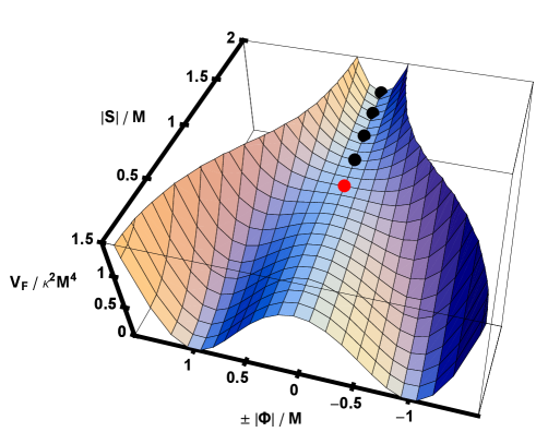
Figure 1: The three dimensional plot of the (dimensionless) F-term potential $V_{\rm F}/\kappa^{2}M^{4}$ for standard FHI versus ${\sf S}=|S|/M~{}~{}\mbox{and}~{}\pm{\sf\Phi}=\pm|\Phi|/M$. The inflationary trajectory is also depicted by black points whereas the critical point by a red/light point.

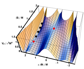
Figure 2: The three dimensional plot of the (dimensionless) F-term potential $V_{\rm F}/\kappa^{2}M^{4}$ for shifted FHI versus ${\sf S}=|S|/M~{}~{}\mbox{and}~{}~{}\pm{\sf\Phi}=\pm|\Phi|/M$ for $\xi=1/6$. The (shifted) inflationary trajectory is also depicted by black points whereas the critical points (of the shifted and standard trajectories) are depicted by red/light points.

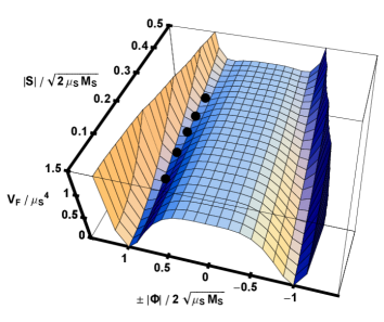
Figure 3: The three dimensional plot of the (dimensionless) F-term potential $V_{\rm F}/\mu_{\rm S}^{4}$ for smooth FHI versus ${\sf S}=|S|/\sqrt{2\mu_{\rm S}M_{\rm S}}~{}~{}\mbox{and}~{}~{}\pm{\sf\Phi}=\pm|\Phi|/2\sqrt{\mu_{\rm S}M_{\rm S}}$. The inflationary trajectory is also depicted by black points.

2.3 The Inflationary Potential

The general form of the potential which can drive the various versions of FHI reads

$$V_{\rm HI}=V_{\rm HI0}+V_{\rm HIc}+V_{\rm HIS}+V_{\rm HIT},~{}~{}\mbox{where:}$$ (6)

• $V_{\rm HI0}$ is the dominant (constant) contribution to $V_{\rm HI}$, which can be written as follows:

  $$V_{\rm HI0}=\left\{\matrix{\kappa^{2}M^{4}\hfill&\mbox{for standard FHI},\hfill\cr\kappa^{2}M_{\xi}^{4}\hfill&\mbox{for shifted FHI},\hfill\cr\mu_{\rm S}^{4}\hfill&\mbox{for smooth FHI},\hfill\cr}\right.$$ (7)

  with $M_{\xi}=M\sqrt{1/4\xi-1}$.

• $V_{\rm HIc}$ is the contribution to $V_{\rm HI}$ which generates a slope along the inflationary valley for driving the inflaton towards the vacua. In the cases of standard [8] and shifted [9] FHI, this slope can be generated by the SUSY breaking on this valley. Indeed, $V_{\rm HI0}>0$ breaks SUSY and gives rise to logarithmic radiative corrections to the potential originating from a mass splitting in the $\Phi-\bar{\Phi}$ supermultiplets. On the other hand, in the case of smooth [10] FHI, the inflationary valleys are not classically flat and, thus, there is no need of radiative corrections. Introducing the canonically normalized inflaton field $\sigma=\sqrt{2}|S|$, $V_{\rm HIc}$ can be written as follows:

  $$V_{\rm HIc}=\left\{\matrix{{\kappa^{4}M^{4}{\sf N}\over 32\pi^{2}}\left(2\ln{\kappa^{2}xM^{2}\over Q^{2}}+f_{c}(x)\right)\hfill&\mbox{for standard FHI},\hfill\cr{\kappa^{4}M_{\xi}^{4}\over 16\pi^{2}}\left(2\ln{\kappa^{2}x_{\xi}M_{\xi}^{2}\over Q^{2}}+f_{c}(x_{\xi})\right)\hfill&\mbox{for shifted FHI,}\hfill\cr-2\mu_{\rm s}^{6}M_{\rm S}^{2}/27\sigma^{4}\hfill&\mbox{for smooth FHI},\hfill\cr}\right.$$ (8)

  $$\mbox{with}~{}f_{c}(x)=(x+1)^{2}\ln(1+1/x)+(x-1)^{2}\ln(1-1/x)\Rightarrow f_{c}(x)\simeq 3~{}~{}\mbox{for}~{}~{}x\gg 1,$$

  $x=\sigma^{2}/2M^{2}$ and $x_{\xi}=\sigma^{2}/M^{2}_{\xi}$. Also ${\sf N}$ is the dimensionality of the representations to which $\bar{\Phi}$ and $\Phi$ belong and $Q$ is a renormalization scale. Although, in some parts (see Sec. 4.3) of our work, rather large $\kappa$’s are used for standard and shifted FHI, renormalization group effects [32] remain negligible.

  In our numerical applications in Secs. 2.6, 3.3, and 4.3 we take ${\sf N}=2$ for standard FHI. This corresponds to the left-right symmetric GUT gauge group $SU(3)_{c}\times SU(2)_{L}\times SU(2)_{R}\times U(1)_{B-L}$ with $\bar{\Phi}$ and $\Phi$ belonging to $SU(2)_{R}$ doublets with $B-L=-1$ and 1 respectively. It is known [14] that no cosmic strings are produced during this realization of standard FHI. As a consequence, we are not obliged to impose extra restrictions on the parameters (as e.g. in Refs. [16, 15]). Let us mention, in passing, that, in the case of shifted [9] FHI, the GUT gauge group is the Pati-Salam group $SU(4)_{c}\times SU(2)_{L}\times SU(2)_{R}$. Needless to say that the case of smooth FHI is independent on the adopted GUT since the inclination of the inflationary path is generated at the classical level and the addition of any radiative correction is expected to be subdominant.

  	Types of FHI
  	Standard	Shifted	Smooth
  The ${\sf\Phi}=0$	Minimum	Minimum	Maximum
  F-flat direction is:	for $|S|\gg M$	for $|S|\gg M$
  Critical point along	Yes	Yes	No
  the inflationary path?	($\sigma_{\rm c}=\sqrt{2}M$)	($\sigma_{\rm c}=M_{\xi}$)
  Classical flatness of	Yes	Yes	No
  the inflationary path?
  Topological defects?	Yes	No	No

  Table 1: Differences and similarities of the various types of FHI.

• $V_{\rm HIS}$ is the SUGRA correction to $V_{\rm HI}$. This emerges if we substitute a specific choice for the Kähler potential $K$ into the SUGRA scalar potential which (without the D-terms) is given by

  $$V_{\rm SUGRA}=e^{K/m_{\rm P}^{2}}\left[(F_{i})^{*}K^{i^{*}j}F_{j}-3\frac{|W|^{2}}{m_{\rm P}^{2}}\right],$$ (9)

  where $F_{i}=W_{i}+K_{i}W/m_{\rm P}^{2}$, a subscript $i~{}[i^{*}]$ denotes derivation with respect to (w.r.t) the complex scalar field $\phi^{i}~{}[\phi^{i}\,{}^{*}]$ and $K^{i^{*}j}$ is the inverse of the matrix $K_{ji^{*}}$. The most elegant, restrictive and highly predictive version of FHI can be obtained, assuming minimal Kähler potential [7, 11], $K_{\rm m}=|S|^{2}$. In such a case $V_{\rm HIS}$ becomes

  $$V_{\rm HISm}=V_{\rm HI0}{\sigma^{4}\over 8m^{4}_{\rm P}},$$ (10)

  where $m_{\rm P}\simeq 2.44\times 10^{18}~{}{\rm GeV}$ is the reduced Planck scale. We can observe that in this case, no other free parameter is added to the initial set of the free parameters of each model (see Sec. 2.6).

• $V_{\rm HIT}$ is the most important contribution to $V_{\rm HI}$ from the soft SUSY effects [15, 17, 33] which can be uniformly parameterized as follows:

  $$V_{\rm HIT}={\rm a}_{S}\sqrt{V_{\rm HI0}}\,\sigma/\sqrt{2}$$ (11)

  where ${\rm a}_{S}$ is of the order of $1~{}{\rm TeV}$. $V_{\rm HIT}$ starts [15, 17, 33] playing an important role in the case of standard FHI for $\kappa\lesssim 5\times 10^{-4}$ and does not have [33], in general, any significant effect in the cases of shifted and smooth FHI.

2.4 Inflationary Observables

Under the assumption that (i) possible deviation from mSUGRA is suppressed (see Sec. 3.2) and (ii) the cosmological scales leave the horizon during FHI and are not reprocessed during a possible subsequent inflationary stage (see Sec. 4), we can apply the standard (see e.g. Refs. [3, 4, 5]) calculations for the inflationary observables of FHI. Namely, we can find:

• The number of e-foldings $N_{\rm HI*}$ that the scale $k_{*}$ suffers during FHI,

  $$N_{\rm HI*}=\>\frac{1}{m^{2}_{\rm P}}\;\int_{\sigma_{\rm f}}^{\sigma_{*}}\,d\sigma\>\frac{V_{\rm HI}}{V^{\prime}_{\rm HI}},$$ (12)

  where the prime denotes derivation w.r.t $\sigma$, $\sigma_{*}$ is the value of $\sigma$ when the scale $k_{*}$ crosses outside the horizon of FHI, and $\sigma_{\rm f}$ is the value of $\sigma$ at the end of FHI, which can be found, in the slow roll approximation, from the condition

  $${\sf max}\{\epsilon(\sigma_{\rm f}),|\eta(\sigma_{\rm f})|\}=1,~{}~{}\mbox{where}~{}~{}\epsilon\simeq{m^{2}_{\rm P}\over 2}\left(\frac{V^{\prime}_{\rm HI}}{V_{\rm HI}}\right)^{2}~{}~{}\mbox{and}~{}~{}\eta\simeq m^{2}_{\rm P}~{}\frac{V^{\prime\prime}_{\rm HI}}{V_{\rm HI}}\cdot$$ (13)

  In the cases of standard [8] and shifted [9] FHI and in the parameter space where the terms in Eq. (10) do not play an important role, the end of inflation coincides with the onset of the GUT phase transition, i.e. the slow roll conditions are violated close to the critical point $\sigma_{\rm c}=\sqrt{2}M$ [$\sigma_{\rm c}=M_{\xi}$] for standard [shifted] FHI, where the waterfall regime commences. On the contrary, the end of smooth [10] FHI is not abrupt since the inflationary path is stable w.r.t $\Phi-\bar{\Phi}$ for all $\sigma$’s and $\sigma_{\rm f}$ is found from Eq. (13).

• The power spectrum $P_{\cal R}$ of the curvature perturbations generated by $\sigma$ at the pivot scale $k_{*}$

  $$P^{1/2}_{\cal R*}=\>\frac{1}{2\sqrt{3}\,\pi m^{3}_{\rm P}}\;\left.\frac{V_{\rm HI}^{3/2}}{|V^{\prime}_{\rm HI}|}\right|_{\sigma=\sigma_{*}}\cdot$$ (14)

• The spectral index

  $$n_{\rm s}=1+\left.{d\ln P_{\cal R}\over d\ln k}\right|_{\sigma=\sigma_{*}}=1-m_{\rm P}^{2}\left.\frac{V_{\rm HI}^{\prime}}{V_{\rm HI}}(\ln P_{\cal R})^{\prime}\right|_{\sigma=\sigma_{*}}=1-6\epsilon_{*}\ +\ 2\eta_{*},$$ (15)

  and its running

  $$\alpha_{\rm s}=\left.{d^{2}\ln P_{\cal R}\over d\ln k^{2}}\right|_{\sigma=\sigma_{*}}={2\over 3}\left(4\eta_{*}^{2}-(n_{\rm s}-1)^{2}\right)-2\xi_{*},$$ (16)

  where $\xi\simeq m_{\rm P}^{4}~{}V^{\prime}_{\rm HI}V^{\prime\prime\prime}_{\rm HI}/V^{2}_{\rm HI}$, the variables with subscript $*$ are evaluated at $\sigma=\sigma_{*}$ and we have used the identity $d\ln k=H\,dt=-d\sigma/\sqrt{2\epsilon}m_{\rm P}$.

We can obtain a rather accurate estimation of the expected $n_{\rm s}$’s if we calculate analytically the integral in Eq. (12) and solve the resulting equation w.r.t $\sigma_{*}$. We pose $\sigma_{f}=\sigma_{\rm c}$ for standard and shifted FHI whereas we solve the equation $\eta(\sigma_{f})=1$ for smooth FHI ignoring $V_{\rm HIS}$. Taking into account that $\epsilon<\eta$ we can extract $n_{\rm s}$ from Eq. (15). In the case of global SUSY – setting $V_{\rm HIS}=V_{\rm HIT}=0$ in Eq. (6) – we find

$$n_{\rm s}=\left\{\matrix{1-{1/N_{\rm HI*}}\hfill&\mbox{for standard and shifted FHI},\hfill\cr 1-{5/3N_{\rm HI*}}\hfill&\mbox{for smooth FHI},\hfill\cr}\right.$$ (17)

whereas in the context of mSUGRA – setting $V_{\rm HIS}=V_{\rm HISm}$ in Eq. (6) – we find

$$n_{\rm s}=\left\{\matrix{1-{1/N_{\rm HI*}}+{3k^{2}{\sf N}N_{\rm HI*}/4\pi^{2}}\hfill&\mbox{for standard FHI},\hfill\cr 1-{1/N_{\rm HI*}}+{3k^{2}N_{\rm HI*}/2\pi^{2}}\hfill&\mbox{for shifted FHI},\hfill\cr 1-{5/3N_{\rm HI*}}+2\left(6\mu^{2}_{\rm S}M^{2}_{\rm S}N_{\rm HI*}/m^{4}_{\rm P}\right)^{1/3}\hfill&\mbox{for smooth FHI}.\hfill\cr}\right.$$ (18)

Comparing the expressions of Eq. (17) and (18), we can easily infer that mSUGRA elevates significantly $n_{\rm s}$ for relatively large $k$ or $M_{\rm S}$.

2.5 Observational Constraints

Under the assumption that (i) the contribution in Eq. (14) is solely responsible for the observed curvature perturbation (for an alternative scenario see Ref. [34]) and (ii) there is a conventional cosmological evolution after FHI (see point (ii) below), the parameters of the FHI models can be restricted imposing the following requirements:

(i)

The power spectrum of the curvature perturbations in Eq. (14) is to be confronted with the WMAP3 data [12]:

$$P^{1/2}_{\cal R*}\simeq\>4.86\times 10^{-5}~{}~{}\mbox{at}~{}~{}k_{*}=0.002/{\rm Mpc}.$$ (19)

(ii)

The number of e-foldings $N_{\rm tot}$ required for solving the horizon and flatness problems of SBB is produced exclusively during FHI and is given by

$$N_{\rm tot}=N_{\rm HI*}\simeq 22.6+{2\over 3}\ln{V^{1/4}_{\rm HI0}\over{1~{}{\rm GeV}}}+{1\over 3}\ln{T_{\rm Hrh}\over{1~{}{\rm GeV}}},$$ (20)

where $T_{\rm Hrh}$ is the reheat temperature after the completion of the FHI.

Indeed, the number of e-foldings $N_{k}$ between horizon crossing of the observationaly relevant mode $k$ and the end of inflation can be found as follows [3]:

$$\frac{k}{H_{0}R_{0}}=\frac{H_{k}R_{k}}{H_{0}R_{0}} = \frac{H_{k}}{H_{0}}\frac{R_{k}}{R_{\rm Hf}}\frac{R_{\rm Hf}}{R_{\rm Hrh}}\frac{R_{\rm Hrh}}{R_{\rm eq}}\frac{R_{\rm eq}}{R_{0}}$$ (21)

$$= \sqrt{V_{\rm HI0}\over{\rho_{\rm c0}}}e^{-N_{k}}\left({V_{\rm HI0}\over\rho_{\rm Hrh}}\right)^{-1/3}\left({\rho_{\rm Hrh}\over\rho_{\rm eq}}\right)^{-1/4}\left({\rho_{\rm eq}\over\rho_{\rm m0}}\right)^{-1/3}$$

$$\Rightarrow N_{k}\simeq\ln{H_{0}R_{0}\over k}+24.72+{2\over 3}\ln{V^{1/4}_{\rm HI0}\over{1~{}{\rm GeV}}}+{1\over 3}\ln{T_{\rm Hrh}\over{1~{}{\rm GeV}}}\cdot$$

Here, $R$ is the scale factor, $H=\dot{R}/R$ is the Hubble rate, $\rho$ is the energy density and the subscripts $0$, $k$, Hf, Hrh, eq and m denote values at the present (except for the symbols $V_{\rm HI0}$ and $H_{\rm HI0}=\sqrt{V_{\rm HI0}}/\sqrt{3}m_{\rm P}$), at the horizon crossing ($k=R_{k}H_{k}$) of the mode $k$, at the end of FHI, at the end of reheating, at the radiation-matter equidensity point and at the matter domination (MD). In our calculation we take into account that $R\propto\rho^{-1/3}$ for decaying-particle domination (DPD) or MD and $R\propto\rho^{-1/4}$ for radiation domination (RD). We use the following numerical values:

$$\rho_{\rm c0}=8.099\times 10^{-47}h_{0}^{2}~{}{\rm GeV^{4}}~{}~{}\mbox{with}~{}~{}h_{0}=0.71,$$

$$\rho_{\rm Hrh}={\pi^{2}\over 30}g_{\rho*}T_{\rm Hrh}^{4}~{}~{}\mbox{with}~{}~{}g_{\rho*}=228.75,$$

$$\rho_{\rm eq}=2\Omega_{\rm m0}(1-z_{\rm eq})^{3}\rho_{\rm c0}~{}~{}\mbox{with}~{}~{}\Omega_{\rm m0}=0.26~{}~{}\mbox{and}~{}~{}z_{\rm eq}=3135.$$ (22)

Setting $H_{0}=2.37\times 10^{-4}/{\rm Mpc}$ and $k/R_{0}=0.002/{\rm Mpc}$ in Eq. (21) we derive Eq. (20).

The cosmological evolution followed in the derivation of Eq. (20) is demonstrated in Fig. 4 where we design the (dimensionless) physical length $\bar{\lambda}_{\rm H0}=\lambda_{\rm H0}/R_{0}$ (dotted line) corresponding to our present particle horizon and the (dimensionless) particle horizon $\bar{R}_{H}=1/\bar{H}=H_{0}/H$ (solid line) versus the logarithmic time $\leavevmode\hbox{\normalsize$\tau$\kern-5.0pt$\iota$}=\ln{R/R_{0}}$. We use $V_{\rm HI0}^{1/4}=10^{15}~{}{\rm GeV}$ and $T_{\rm Hrh}=10^{9}~{}{\rm GeV}$ (which result to $N_{\rm HI*}\simeq 55$). We take into account that $\ln\bar{\lambda}\propto\leavevmode\hbox{\normalsize$\tau$\kern-5.0pt$\iota$}$, $\bar{R}_{H}=H_{0}/H_{\rm HI0}$ for FHI and $\ln\bar{R}_{H}\propto 2\leavevmode\hbox{\normalsize$\tau$\kern-5.0pt$\iota$}~{}[\ln\bar{R}_{H}\propto 1.5\leavevmode\hbox{\normalsize$\tau$\kern-5.0pt$\iota$}]$ for RD [MD]. The various eras of the cosmological evolution are also clearly shown.

Fig. 4 visualizes [5] the resolution of the horizon problem of SBB with the use of FHI. Indeed, suppose that $\bar{\lambda}_{\rm H0}$ (which crosses the horizon today, $\bar{\lambda}_{\rm H0}(0)=\bar{R}_{H}(0)$) indicates the distance between two photons we detect in CMB. In the absence of FHI, the observed homogeneity of CMB remains unexplained since $\lambda_{\rm H0}$ was outside the horizon, $(\bar{\lambda}_{\rm H0}/\bar{R}_{H})(\leavevmode\hbox{\normalsize$\tau$\kern-5.0pt$\iota$}_{\rm LS})\simeq 33.11$, at the time of last-scattering (LS) (with temperature $T_{\rm LS}\simeq 0.26~{}{\rm eV}$ or logarithmic time $\leavevmode\hbox{\normalsize$\tau$\kern-5.0pt$\iota$}_{\rm LS}\simeq-7$) when the two photons were emitted and so, they could not establish thermodynamic equilibrium. There were $3.6\times 10^{4}$ disconnected regions within the volume $\bar{\lambda}_{\rm H0}^{3}(\leavevmode\hbox{\normalsize$\tau$\kern-5.0pt$\iota$}_{\rm LS})$. In other words, photons on the LS surface (with radius $\bar{R}_{H}(0)$) separated by an angle larger than $\theta=\bar{\lambda}_{\rm LS}(0)/\bar{R}_{H}(0)\simeq(1/33.11)~{}{\rm rad}=1.7^{0}$ were not in casual contact – here, $\lambda_{\rm LS}$ is the physical length which crossed the horizon at LS. On the contrary, in the presence of FHI, $\lambda_{\rm H0}$ has a chance to be within the horizon again, $\bar{\lambda}_{\rm H0}<\bar{R}_{H}$, if FHI produces around $56$ e-foldings before its termination. If this happens, the homogeneity and the isotropy of CMB can be easily explained: photons that we receive today and were emitted from causally disconnected regions of the LS surface, have the same temperature because they had a chance to communicate to each other before FHI.

Figure 4: The evolution of the quantities $1/\bar{H}=H/H_{0}$ with (solid line) and $\bar{\lambda}_{\rm H0}=\lambda/R_{0}$ (dotted line) as a function of $\tau$$\iota$ for $V_{\rm HI0}^{1/4}=10^{15}~{}{\rm GeV}$, $N_{\rm HI*}\simeq 55$ and $T_{\rm Hrh}=10^{9}~{}{\rm GeV}$. The various eras of the cosmological evolution are also shown.

2.6 Numerical Results

Our numerical investigation depends on the parameters:

$$\sigma_{*},v_{{}_{G}}~{}~{}\mbox{and}\left\{\matrix{\kappa\hfill&\mbox{for standard FHI},\hfill\cr\kappa~{}~{}\mbox{with fixed}~{}~{}M_{\rm S}=5\times 10^{17}~{}{\rm GeV}\hfill&\mbox{for shifted FHI},\hfill\cr M_{\rm S}\hfill&\mbox{for smooth FHI}.\hfill\cr}\right.$$

In our computation, we use as input parameters $\kappa$ or $M_{\rm S}$ and $\sigma_{*}$ and we then restrict $v_{{}_{G}}$ and $\sigma_{*}$ so as Eqs. (19) and (20) are fulfilled. Using Eqs. (15) and (16) we can extract $n_{\rm s}$ and $\alpha_{\rm s}$ respectively which are obviously predictions of each FHI model – without the possibility of fulfilling Eq. (1) by some adjustment.

In the case of standard FHI with ${\sf N}=2$, we present the allowed by Eqs. (19) and (20) values of $v_{{}_{G}}$ versus $\kappa$ (Fig. 5) and $n_{\rm s}$ versus $\kappa$ (Fig. 6). Dashed [solid] lines indicate results obtained within SUSY [mSUGRA], i.e. by setting $V_{\rm HIS}=V_{\rm HIT}=0$ [$V_{\rm HIS}=V_{\rm HISm}$ given by Eq. (10) and $V_{\rm HIT}$ given by Eq. (11) with a_S=1 TeV] in Eq. (6). We, thus, can easily identify the regimes where the several contributions to $V_{\rm HI}$ dominate. Namely, for $\kappa\gtrsim 0.01$, $V_{\rm HISm}$ dominates and drives $n_{\rm s}$ to values close to or larger than unity – see Fig. 6. On the other hand, for $5\times 10^{-4}\lesssim\kappa\lesssim 0.01$, $V_{\rm HIc}$ becomes prominent. Finally, for $\kappa\lesssim 5\times 10^{-3}$, $V_{\rm HIT}$ starts playing an important role and as $v_{{}_{G}}$ increases, $V_{\rm HISm}$ becomes again important. In Fig. 6 we also design with thin lines the region of Eq. (1). We deduce that there is a marginally allowed area with $0.983\lesssim n_{\rm s}\lesssim 0.99$. This occurs for

$$0.0015\lesssim\kappa\lesssim 0.03~{}~{}\mbox{with}~{}~{}0.56\lesssim v_{{}_{G}}/(10^{16}~{}{\rm GeV})\lesssim 0.74.$$

in mSUGRA whereas in global SUSY we have $\kappa\gtrsim 0.0015$ and $0.56\lesssim v_{{}_{G}}/(10^{16}~{}{\rm GeV})$ $\lesssim 0.7$. We realize that $v_{{}_{G}}<M_{\rm GUT}$ – note that $M_{\rm GUT}=(2\times 10^{16}/0.7)~{}{\rm GeV}$ where $2\times 10^{16}~{}{\rm GeV}$ is the mass acquired by the gauge bosons during the SUSY GUT breaking and $0.7$ is the unified gauge coupling constant at the scale $2\times 10^{16}~{}{\rm GeV}$.

In the cases of shifted and smooth FHI we confine ourselves to the values of the parameters which give $v_{{}_{G}}=M_{\rm GUT}$ and display the solutions consistent with Eqs. (19) and (20) in Table 2. We observe that the required $\kappa$ in the case of shifted FHI is rather low and so, the inclusion of mSUGRA does not raise $n_{\rm s}$, which remains within the range of Eq. (1). On the contrary, in the case of smooth FHI, $n_{\rm s}$ increases sharply within mSUGRA although the result in the absence of mSUGRA is slightly lower than this of shifted FHI. In the former case $|\alpha_{\rm s}|$ is also considerably enhanced.

Shifted FHI			Smooth FHI
	Without	With		Without	With
	mSUGRA			mSUGRA
$\kappa/10^{-3}$	$9.2$		$M_{\rm S}/5\times 10^{17}~{}{\rm GeV}$	$1.56$	$0.79$
$\sigma_{*}/10^{16}~{}{\rm GeV}$	$5.37$		$\sigma_{*}/10^{16}~{}{\rm GeV}$	$26.8$	$32.9$
$M/10^{16}~{}{\rm GeV}$	$2.3$		$\mu_{\rm S}/10^{16}~{}{\rm GeV}$	$0.1$	$0.21$
$1/\xi$	$4.36$		$\sigma_{\rm f}/10^{16}~{}{\rm GeV}$	$13.4$	$13.4$
$N_{\rm HI*}$	$52.2$		$N_{\rm HI*}$	$52.5$	$53$
$n_{\rm s}$	$0.982$		$n_{\rm s}$	$0.969$	$1.04$
$-\alpha_{\rm s}/10^{-4}$	$3.4$		$-\alpha_{\rm s}/10^{-4}$	$5.8$	$16.6$

Table 2: Input and output parameters consistent with Eqs. (19) and (20) for shifted ($M_{\rm S}=5\times 10^{17}~{}{\rm GeV}$) or smooth FHI and $v_{{}_{G}}=M_{\rm GUT}$ with and without the mSUGRA contribution.

Figure 5: The allowed by Eqs. (19) and (20) values of $v_{{}_{G}}$ versus $\kappa$ for standard FHI with ${\sf N}=2$ and $V_{\rm HIS}={\rm a}_{S}=0$ (dashed lines) or $V_{\rm HIS}=V_{\rm HISm}$ and a${}_{S}=1~{}{\rm TeV}$ (solid lines).

Figure 6: The allowed by Eqs. (19) and (20) values of $n_{\rm s}$ versus $\kappa$ for standard FHI with ${\sf N}=2$ and $V_{\rm HIS}={\rm a}_{S}=0$ (dashed lines) or $V_{\rm HIS}=V_{\rm HISm}$ and a${}_{S}=1~{}{\rm TeV}$ (solid lines). The region of Eq. (1) is also limited by thin lines.

3 Reducing $n_{s}$ Through Quasi-Canonical SUGRA

Sizeable variation of $n_{\rm s}$ in FHI can be achieved by considering a moderate deviation from mSUGRA, named [19] qSUGRA. The form of the relevant Kähler potential for $\sigma$ is given by

$$K_{\rm q}=\ {\sigma^{2}\over 2}\pm\ c_{\rm q}\;{\sigma^{4}\over 4m^{2}_{\rm P}}$$ (23)

with $c_{\rm q}>0$ a free parameter. Note that for $\sigma\ll m_{\rm P}$ higher order terms in the expansion of Eq. (23) have no effect on the inflationary dynamics. Inserting Eq. (23) into Eq. (9), we obtain the corresponding contribution to $V_{\rm HI}$,

$$V_{\rm HISq}\simeq V_{\rm HI0}\left(\mp c_{\rm q}\frac{\sigma^{2}}{2m^{2}_{\rm P}}+c_{\rm qq}\frac{\sigma^{4}}{8m^{4}_{\rm P}}\>+\>{\cal O}\left({\sigma\over m_{\rm P}}\right)^{6}\right)~{}~{}\mbox{with}~{}~{}c_{\rm qq}=1-{7\over 2}c_{\rm q}+{5\over 2}c_{\rm q}^{2}.$$ (24)

The fitting of WMAP3 data by $\Lambda$CDM model obliges [17, 18, 21] us to consider the positive [minus] sign in Eq. (23) [Eq. (24)] (the opposite choice implies [19] a pronounced increase of $n_{\rm s}$ above unity). As a consequence $V_{\rm HI}$ acquires a rather interesting structure which is studied in Sec. 3.1. In Sec. 3.2 we specify the observational constraints which we impose to this scenario and in Sec. 3.3 we exhibit our numerical results.

3.1 The Structure of the Inflationary Potential

In the qSUGRA scenario the potential $V_{\rm HI}$ can be derived from Eq. (6) posing $V_{\rm HIS}=V_{\rm HISq}$ given by Eq. (24) with minus in the first term. Depending on the value of $c_{\rm q}$, $V_{\rm HI}$ is a monotonic function of $\sigma$ or develops a local minimum and maximum. The latter case leads to two possible complications: (i) The system gets trapped near the minimum of $V_{\rm HI}$ and, consequently, no FHI takes place and (ii) even if FHI of the so-called hilltop type [20] occurs with $\sigma$ rolling from the region of the maximum down to smaller values, a mild tuning of the initial conditions is required [17] in order to obtain acceptable $n_{\rm s}$’s.

It is, therefore, crucial to check if we can accomplish the aim above, avoiding [21, 22] the minimum-maximum structure of $V_{\rm HI}$. In such a case the system can start its slow rolling from any point on the inflationary path without the danger of getting trapped. This can be achieved, if we require that $V_{\rm HI}$ is a monotonically increasing function of $\sigma$, i.e. $V^{\prime}_{\rm HI}>0$ for any $\sigma$ or, equivalently,

$$V^{\prime}_{\rm HI}(\bar{\sigma}_{\rm min})>0~{}~{}\mbox{with}~{}~{}V^{\prime\prime}_{\rm HI}(\bar{\sigma}_{\rm min})=0~{}~{}\mbox{and}~{}~{}V^{\prime\prime\prime}_{\rm HI}(\bar{\sigma}_{\rm min})>0$$ (25)

where $\bar{\sigma}_{\rm min}$ is the value of $\sigma$ at which the minimum of $V^{\prime}_{\rm HI}$ lies. Employing the conditions of Eq. (25) we find approximately:

$$\bar{\sigma}_{\rm min}\simeq\left\{\matrix{\sqrt{2c_{\rm q}/3c_{\rm qq}}\;m_{\rm P}\hfill&\mbox{for standard and shifted FHI},\hfill\cr\sqrt{2m_{\rm P}/3}\left(\sqrt{5/c_{\rm qq}}\;\mu_{\rm S}M_{\rm S}\right)^{1/4}\hfill&\mbox{for smooth FHI}.\hfill\cr}\right.$$ (26)

Inserting Eq. (26) into Eq. (25), we find that $V_{\rm HI}$ remains monotonic for

$$c_{\rm q}<c_{\rm q}^{\rm max}~{}~{}\mbox{with}~{}~{}c_{\rm q}^{\rm max}=\left\{\matrix{{3\kappa\sqrt{c_{\rm qq}{\sf N}}/4\sqrt{2}\pi}\hfill&\mbox{for standard FHI},\hfill\cr{3\kappa\sqrt{c_{\rm qq}}/4\pi}\hfill&\mbox{for shifted FHI},\hfill\cr(8/3)(c_{\rm qq}/5)^{3/4}\sqrt{\mu_{\rm S}M_{\rm S}}/m_{\rm P}\hfill&\mbox{for smooth FHI}.\hfill\cr}\right.$$ (27)

For $c_{\rm q}>c_{\rm q}^{\rm max}$, $V_{\rm HI}$ reaches at the points $\sigma_{\rm min}$ [$\sigma_{\rm max}$] a local minimum [maximum] which can be estimated as follows:

$$\sigma_{\rm min}\simeq\sqrt{2c_{\rm q}\over c_{\rm qq}}m_{\rm P}~{}~{}\mbox{and}~{}~{}\sigma_{\rm max}\simeq\left\{\matrix{\kappa m_{\rm P}\sqrt{\sf N}/2\sqrt{2c_{\rm q}}\pi\hfill&\mbox{for standard FHI},\hfill\cr{\kappa m_{\rm P}/2\sqrt{c_{\rm q}}\pi}\hfill&\mbox{for shifted FHI},\hfill\cr\sqrt{2/3c_{\rm q}}{\left(\mu_{\rm S}M_{\rm S}m_{\rm P}\right)^{1/3}}\hfill&\mbox{for smooth FHI}.\hfill\cr}\right.$$ (28)

Even in this case, the system can always undergo FHI starting at $\sigma<\sigma_{\rm max}$ since $V^{\prime}_{\rm HI}(\sigma_{\rm max})=0$. However, the lower $n_{\rm s}$ we want to obtain, the closer we must set $\sigma_{*}$ to $\sigma_{\rm max}$. This signalizes [17] a substantial tuning in the initial conditions of FHI.

Employing the strategy outlined in Sec. (2.4) we can take a flavor for the expected $n_{\rm s}$’s in the qSUGRA scenario, for any $c_{\rm q}$:

$$n_{\rm s}=\left\{\matrix{1-2c_{\rm q}\left(1-1/c_{N}\right)-{3c_{\rm qq}\kappa^{2}{\sf N}c_{N}/4c_{\rm q}\pi^{2}}\hfill&\mbox{for standard FHI},\hfill\cr 1-2c_{\rm q}\left(1-1/c_{N}\right)-{3c_{\rm qq}\kappa^{2}c_{N}/4c_{\rm q}\pi^{2}}\hfill&\mbox{for shifted FHI},\hfill\cr 1-5/3N_{\rm HI*}+2\tilde{c}_{N}-\left(2\tilde{c}_{N}N_{\rm HI*}+7\right)c_{\rm q}\hfill&\mbox{for smooth FHI},\hfill\cr}\right.$$ (29)

$$\mbox{with}~{}~{}c_{N}=1-\sqrt{1+4c_{\rm q}N_{\rm HI*}}~{}~{}\mbox{and}~{}~{}\tilde{c}_{N}=c_{\rm qq}\left(6\mu^{2}_{\rm S}M^{2}_{\rm S}N_{\rm HI*}/m^{4}_{\rm P}\right)^{1/3}.$$

We can clearly appreciate the contribution of a positive $c_{\rm q}$ to the lowering of $n_{\rm s}$.

3.2 Observational Constraints

As in the case of mSUGRA and under the same assumptions, the qSUGRA scenario needs to satisfy Eq. (19) and (20). However, due to the presence of the extra parameter $c_{\rm q}$, a simultaneous fulfillment of Eq. (1) becomes [18, 17, 21] possible. In addition, we take into account, as optional constraint, Eq. (25) so as complications from the appearance of the minimum-maximum structure of $V_{\rm HI}$ are avoided.

It is worth mentioning that $K_{\rm q}$ in Eq. (23) generates a non-minimal kinetic term of $\sigma$ thereby altering, in principle, the inflationary dynamics and the calculation of the inflationary observables. Indeed, the kinetic term of $\sigma$ is

$${1\over 2}{\partial^{2}K_{\rm q}\over\partial S\partial S^{*}}\dot{\sigma}^{2}~{}~{}\mbox{with}~{}~{}{\partial^{2}K_{\rm q}\over\partial S\partial S^{*}}=1\pm 2c_{\rm q}{\sigma^{2}\over m_{\rm P}^{2}}$$ (30)

(the dot denotes derivation w.r.t the cosmic time). Assuming that the ‘friction’ term $3H\dot{\sigma}$ dominates over the other terms in the equation of motion (e.o.m) of $\sigma$, we can derive the slow roll parameters $\epsilon$ and $\eta$ in Eq. (13) which carry an extra factor $(1\pm 2c_{\rm q}\sigma^{2}/m_{\rm P}^{2})^{-1}$, in the present case. The formulas in Eqs. (12) and (14) get modified also. In particular, a factor $(1\pm 2c_{\rm q}\sigma^{2}/m_{\rm P}^{2})$ must be included in the integrand in the right-hand side (r.h.s) of Eq. (12) and a factor $(1\pm 2c_{\rm q}\sigma^{2}/m_{\rm P}^{2})^{1/2}$ in the r.h.s of Eq. (14). However, these modifications are certainly numerically negligible since $\sigma\ll m_{\rm P}$ and $c_{\rm q}\ll 1$ (see Sec. 3.3).

3.3 Numerical Results

Shifted FHI				Smooth FHI
$n_{\rm s}$	$0.926$	$0.958$	$0.976$	$n_{\rm s}$	$0.926$	$0.958$	$0.99$
$c_{\rm q}/10^{-3}$	$16.8$	$7.5$	$2$	$c_{\rm q}/10^{-3}$	$11$	$8.3$	$5.45$
$c^{\rm max}_{\rm q}/10^{-3}$	$1.7$	$1.87$	$2$	$c^{\rm max}_{\rm q}/10^{-3}$	$9$	$9$	$9$
$\sigma_{*}/10^{16}~{}{\rm GeV}$	$6.05$	$5.46$	$5.36$	$\sigma_{*}/10^{16}~{}{\rm GeV}$	$23.1$	$24.5$	$26.5$
$\kappa/10^{-3}$	$7.8$	$8.45$	$9$	$M_{\rm S}/5\times 10^{17}~{}{\rm GeV}$	$2.86$	$2.02$	$1.44$
$M/10^{16}~{}{\rm GeV}$	$2.18$	$2.24$	$2.28$	$\mu_{\rm S}/10^{16}~{}{\rm GeV}$	$0.06$	$0.08$	$0.1$
$1/\xi$	$4.1$	$4.21$	$4.31$	$\sigma_{\rm f}/10^{16}~{}{\rm GeV}$	$13.4$	$13.4$	$13.4$
$N_{\rm HI*}$	$51.7$	$52$	$52$	$N_{\rm HI*}$	$52.2$	$52.4$	$52.6$
$-\alpha_{\rm s}/10^{-4}$	$2.8$	$3.4$	$3.5$	$-\alpha_{\rm s}/10^{-3}$	$0.56$	$0.8$	$1$

Table 3: Input and output parameters consistent with Eqs. (19) and (20) for shifted ($M_{\rm S}=5\times 10^{17}~{}{\rm GeV}$) or smooth FHI, $v_{{}_{G}}=M_{\rm GUT}$ and selected $n_{\rm s}$’s within the qSUGRA scenario.

Our strategy in the numerical investigation of the qSUGRA scenario is the one described in Sec. 2.6. In addition to the parameters manipulated there, here we have the parameter $c_{\rm q}$ which can be adjusted so as to achieve $n_{\rm s}$ in the range of Eq. (1). We check also the fulfillment of Eq. (25).

In the case of standard FHI with ${\sf N}=2$, we delineate the (lightly gray shaded) region allowed by Eqs. (1), (19) and (20) in the $\kappa-c_{\rm q}$ (Fig. 7) and $\kappa-v_{{}_{G}}$ (Fig. 8) plane. The conventions adopted for the various lines are also shown in the r.h.s of each graphs. In particular, the black solid [dashed] lines correspond to $n_{\rm s}=0.99$ [$n_{\rm s}=0.926$], whereas the gray solid lines have been obtained by fixing $n_{\rm s}=0.958$ – see Eq. (1). The dot-dashed lines correspond to $c_{\rm q}=c_{\rm q}^{\rm max}$ in Eq. (27) whereas the dotted line indicates the region in which Eq. (1) is fulfilled in the mSUGRA scenario. In the hatched region, Eq. (25) is also satisfied. We observe that the optimistic constraint of Eq. (25) can be met in a narrow but not unnaturaly small fraction of the allowed area. Namely, for $n_{\rm s}=0.958$, we find

$$0.06\lesssim\kappa\lesssim 0.15~{}~{}\mbox{with}~{}~{}0.47\gtrsim v_{{}_{G}}/(10^{16}~{}{\rm GeV})\gtrsim 0.37~{}~{}\mbox{and}~{}~{}0.013\lesssim c_{\rm q}\lesssim 0.03.$$

The lowest $n_{\rm s}=0.946$ can be achieved for $\kappa=0.15$. Note that the $v_{{}_{G}}$’s encountered here are lower that those found in the mSUGRA scenario (see Sec. 2.6).

In the cases of shifted and smooth FHI we confine ourselves to the values of the parameters which give $v_{{}_{G}}=M_{\rm GUT}$ and display in Table 3 their values which are also consistent with Eqs. (19) and (20) for selected $n_{\rm s}$’s. In the case of shifted FHI, we observe that (i) it is not possible to obtain $n_{\rm s}=0.99$ since the mSUGRA result is lower (see Table 2) (ii) the lowest possible $n_{\rm s}$ compatible with the conditions of Eq. (25) is $0.976$ and so, $n_{\rm s}=0.958$ is not consistent with Eq. (25). In the case of smooth FHI, we see that reduction of $n_{\rm s}$ consistently with Eq. (25) can be achieved for $n_{\rm s}\gtrsim 0.951$ and so $n_{\rm s}=0.958$ can be obtained without complications.

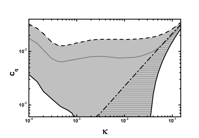
Figure 7: Allowed (lightly gray shaded) region in the $\kappa-c_{\rm q}$ plane for standard FHI within the qSUGRA scenario. Ruled is the region where the inflationary potential remains monotonic. The conventions adopted for the various lines are also shown.

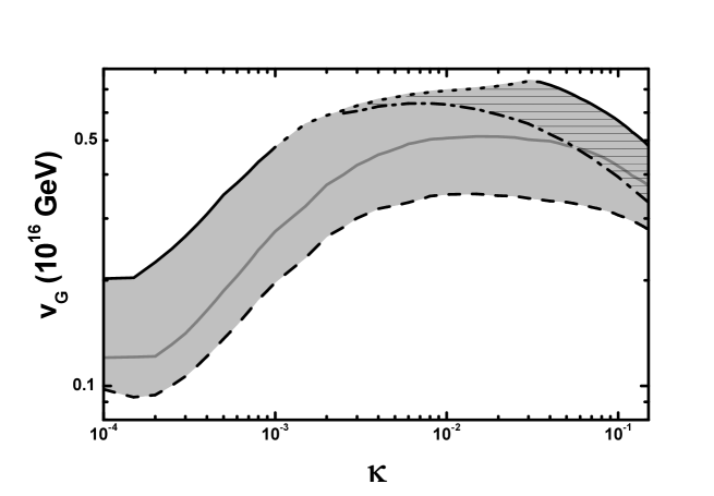
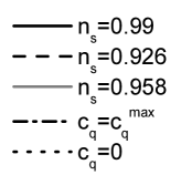
Figure 8: Allowed (lightly gray shaded) region in the $\kappa-v_{{}_{G}}$ plane for standard FHI within the qSUGRA scenario. Ruled is the region where the inflationary potential remains monotonic. The conventions adopted for the various lines are also shown.

4 Reducing $n_{s}$ Through a Complementary MI

Another, more drastic and radical, way to circumvent the $n_{s}$ problem of FHI is the consideration of a double inflationary set-up. This proposition [23] is based on the observation that $n_{\rm s}$ within FHI models generally decreases [32] with $N_{\rm HI*}$ – given by Eq. (12). This statement is induced by Eqs. (17) and (18) and can be confirmed by Fig. 9 where we draw $n_{\rm s}$ in standard FHI with ${\sf N}=1$ as a function of $N_{\rm HI*}$ for several $\kappa$’s indicated in the graph. On the curves, Eq. (19) is satisfied. Therefore, we could constrain $N_{\rm HI*}$, fulfilling Eq. (1). Note that a constrained $N_{\rm HI*}$ was also previously used in Ref. [35] to achieve a sufficient running of $n_{\rm s}$.

The residual amount of e-foldings, required for the resolution of the horizon and flatness problems of the standard big-bang cosmology, can be generated during a subsequent stage of MI realized at a lower scale by a string modulus. We show that this scenario can satisfy a number of constraints with more or less natural values of the parameters. Such a construction is also beneficial for MI, since the perturbations of the inflaton field in this model are not sufficiently large to account for the observations, due to the low inflationary energy scale.

Let us also mention that MI naturally assures a low reheat temperature. As a consequence, the gravitino constraint [30] on the reheat temperature of FHI and the potential topological defect problem of standard FHI [31] can be significantly relaxed or completely evaded. On the other hand, for the same reason baryogenesis is made more difficult, since any preexisting baryon asymmetry is diluted by the entropy production during the modulus decay. However, it is not impossible to achieve adequate baryogenesis in the scheme of cold electroweak baryogenesis [36] or in the context of (large) extra dimensions [37].

The main features of MI are sketched in Sec. 4.1. The parameter space of the present scenario is restricted in Sec. 4.3 taking into account a number of observational requirements which are exhibited in Sec. 4.2

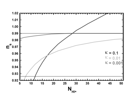
Figure 9: The spectral index $n_{\rm s}$ in standard FHI as a function of $N_{\rm HI*}$ for several $\kappa$’s indicated in the graph. On the curves, Eq. (19) is satisfied.

4.1 The Basics of MI

Fields having (mostly Planck scale) suppressed couplings to the SM degrees of freedom and weak scale (non-SUSY) mass are called collectively moduli. After the gravity mediated soft SUSY breaking, their potential can take the form (see the appendix A in Ref. [38]):

$$V_{\rm MI}=(m_{3/2}m_{\rm P})^{2}{\cal V}\left({s\over m_{\rm P}}\right)$$ (31)

where ${\cal V}$ is a function with dimensionless coefficients of order unity and $s$ is the canonically normalized, axionic or radial component of a string modulus. MI is usually supposed [24] to take place near a maximum of $V_{\rm MI}$, which can be expanded as follows:

$$V_{\rm MI}\simeq V_{\rm MI0}-\frac{1}{2}m_{s}^{2}s^{2}+\cdots,$$ (32)

where the ellipsis denotes terms which are expected to stabilize $V_{\rm MI}$ at $s\sim m_{\rm P}$. Comparing Eqs. (31) and (32), we conclude that

$$V_{\rm MI0}=v_{s}(m_{3/2}m_{\rm P})^{2}~{}~{}{\rm and}~{}~{}m_{s}\sim m_{3/2},$$ (33)

where $m_{3/2}\sim 1~{}{\rm TeV}$ is the gravitino mass and the coefficient $v_{s}$ is of order unity, yielding $V_{\rm MI0}^{1/4}\simeq 3\times 10^{10}~{}{\rm GeV}$. However, if $s$ has just Plank scale suppressed interactions to light degrees of freedom, NS constraint forces [44] us to use (see Sec. 4.2) much larger values for $m_{s}$ and $m_{3/2}$. In Fig. 10, we present a typical example of the (dimensionless) potential $V_{\rm MI}/(m_{3/2}m_{\rm P})^{2}$ versus $s/m_{\rm P}$, where the constant quantity $c_{\rm MI0}\simeq 0.7$ has been subtracted so that $V_{\rm MI}/(m_{3/2}m_{\rm P})^{2}$ vanishes at its absolute minimum (the subscript $0$ of $V_{\rm MI0}$ and $c_{\rm MI0}$ is not refereed to present-day values).

Figure 10: The (dimensionless) potential $V_{\rm MI}/(m_{3/2}m_{\rm P})^{2}=1-0.5(s/m_{\rm P})^{2}+0.2(s/m_{\rm P})^{4}-c_{\rm MI0}$ versus $s/m_{\rm P}$. The inflationary trajectory is also depicted by black points.

Solving the e.o.m of the field $s$ (the dot denotes derivation w.r.t the cosmic time),

$$\ddot{s}+3Hs+d^{2}V/ds^{2}=0,$$ (34)

for $H=H_{s}\simeq\sqrt{V_{\rm MI0}}/\sqrt{3}m_{\rm P}$ and $V=V_{\rm MI}\Rightarrow d^{2}V/ds^{2}\simeq-m^{2}_{s}$, we can extract [28] its evolution during MI:

$$s=s_{\rm Mi}e^{F_{s}\Delta N_{\rm MI}}~{}~{}\mbox{with}~{}~{}F_{s}\equiv\sqrt{{9\over 4}+\left(\frac{m_{s}}{H_{s}}\right)^{2}}-{3\over 2}\cdot$$ (35)

Here, $s_{\rm Mi}$ is the value of $s$ at the onset of MI and $\Delta N_{\rm MI}$ is the number of the e-foldings obtained from $s=s_{\rm Mi}$ until a given $s$. For natural MI we need:

$$0.5\leq v_{s}\leq 10~{}~{}\Rightarrow~{}~{}2.45\geq m_{s}/H_{s}\geq 0.55~{}~{}\Rightarrow~{}~{}1.37\geq F_{s}\geq 0.097.$$ (36)

where the lower bound bound on $v_{s}$ comes from the obvious requirement $V_{\rm MI}>0$.

In this model, inflation can be not only of the slow-roll but also of the fast-roll [28] type. This is, because there is a range of parameters where, although the $\epsilon$-criterion for MI, $\epsilon_{s}<1$, is fulfilled, the $\eta$-criterion, $\eta_{s}<1$, is violated giving rise to fast-roll inflation. Indeed, using its most general form [5], $\epsilon_{s}$ reads:

$$\epsilon_{s}=-{\dot{H}_{\rm MI}\over H_{\rm MI}^{2}}=F_{s}^{2}{s^{2}\over 2m^{2}_{\rm P}},$$ (37)

where the former expression can be derived inserting Eq. (35) into Eq. (34) with $H=H_{\rm MI}=\sqrt{V_{\rm MI}}/\sqrt{3}m_{\rm P}$. Numerically we find:

$$0.005\leq\epsilon_{s}\leq 0.94~{}~{}\mbox{for}~{}~{}0.55\leq m_{s}/H_{s}\leq 2.45~{}~{}\mbox{and}~{}~{}s/m_{\rm P}=1.$$ (38)

Therefore, we can obtain accelerated expansion (i.e. inflation) with $H_{s}\simeq\rm{cst}$. Note, though, that near the upper bound on $m_{s}/H_{s}$, $\epsilon_{s}$ gets too close to unity at $s=m_{\rm P}$ and thus, $H_{s}$ does not remain constant as $s$ approaches $m_{\rm P}$. Therefore, our results at large values of $m_{s}/H_{s}$ should be considered only as indicative. On the other hand, $\eta_{s}$ can be larger or lower than 1, since:

$$|\eta_{s}|=m^{2}_{\rm P}{|d^{2}V_{\rm MI}/ds^{2}|\over V_{\rm MI}}={m_{s}^{2}\over 3H_{s}^{2}}\simeq{1\over v_{s}}$$ (39)

where the last equality holds for $m_{s}=m_{3/2}$. Therefore, the condition which discriminates the slow-roll from the fast-roll MI is:

$$\left\{\matrix{m_{s}/H_{s}<\sqrt{3}\hfill&\mbox{or}~{}~{}v_{s}>1&\mbox{for slow-roll MI},\hfill\cr m_{s}/H_{s}>\sqrt{3}\hfill&\mbox{or}~{}~{}v_{s}<1&\mbox{for fast-roll MI}.\hfill\cr}\right.$$ (40)

Figure 11: The number of e-foldings $N_{\rm MI}$ obtained during MI as a function of $m_{s}/H_{s}$ for $s_{\rm Mf}/m_{\rm P}=1$ and several $s_{i}/m_{\rm P}$’s indicated in the graph. The required values of $N_{\rm MI}$ for a successful complementary MI is approximately limited by two thin line.

The total number of $e$-foldings during MI can be found from Eq. (35). Namely,

$$N_{\rm MI}=\frac{1}{F_{s}}\ln{s_{\rm Mf}\over s_{\rm Mi}}\simeq\frac{1}{F_{s}}\ln\frac{m_{\rm P}}{s_{\rm Mi}}\cdot$$ (41)

In our computation we take for the value of $s$ at the end of MI $s_{\rm Mf}=m_{\rm P}$, since the condition $\epsilon_{s}=1$ gives $s_{\rm Mf}/m_{\rm P}=\sqrt{2}/F_{s}>1$, for the ranges of Eq. (36). This result is found because the (unspecified) terms in the ellipsis in the r.h.s of Eq. (32) starts playing an important role for $s\sim m_{\rm P}$ and it is obviously unacceptable.

In Fig. 11, we depict $N_{\rm MI}$ versus $m_{s}/H_{s}$ for $s_{\rm Mf}=m_{\rm P}$ and several $s_{\rm Mi}/m_{\rm P}$’s indicated in the graph. We observe that $N_{\rm MI}$ is very sensitive to the variations of $m_{s}/H_{s}$. Also, taking into account that $20\lesssim N_{\rm MI}\lesssim 30$ (limited in Fig. 11 by two thin lines) is needed so that MI plays successfully the role of complementary inflation (see Sec. 4.3), we can deduce the following:

• As $s_{\rm Mi}$ decreases, the required $m_{s}/H_{s}$ for obtaining $N_{\rm MI}\sim 30$ increases. To this end, for $s_{\rm Mi}/m_{\rm P}\lesssim 10^{-8}$ [$s_{\rm Mi}/m_{\rm P}\gtrsim 10^{-8}$], we need fast-roll [slow-roll] MI.

• For $s_{\rm Mi}/m_{\rm P}\gtrsim 0.1$, it is not possible to obtain $N_{\rm MI}\sim 30$ and so, MI can not play successfully the role of complementary inflation.

4.2 Observational Constraints

In addition to Eqs. (1) and (19) – on the assumption that the inflaton perturbation generates exclusively the curvature perturbation – the cosmological scenario under consideration needs to satisfy a number of other constraints too. These can be outlined as follows:

(i)

The horizon and flatness problems of SBB can be successfully resolved provided that the scale $k_{*}$ suffered a certain total number of e-foldings $N_{\rm tot}$. In the present set-up, $N_{\rm tot}$ consists of two contributions:

$$N_{\rm tot}=N_{\rm HI*}+N_{\rm MI}\,.$$ (42)

Employing the conventions and the strategy we applied in the derivation of Eq. (21), we can find [39] the number of e-foldings $N_{k}$ between horizon crossing of the observationaly relevant mode $k$ and the end of FHI as follows:

$$\frac{k}{H_{0}R_{0}} = \frac{H_{k}R_{k}}{H_{0}R_{0}}$$ (43)

$$= \frac{H_{k}}{H_{0}}\frac{R_{k}}{R_{\rm Hf}}\frac{R_{\rm Hf}}{R_{\rm Mi}}\frac{R_{\rm Mi}}{R_{\rm Mf}}\frac{R_{\rm Mf}}{R_{\rm Mrh}}\frac{R_{\rm Mrh}}{R_{\rm eq}}\frac{R_{\rm eq}}{R_{0}}$$

$$= \sqrt{V_{\rm HI0}\over{\rho_{\rm c0}}}e^{-N_{k}}\left({V_{\rm HI0}\over V_{\rm MI0}}\right)^{-1/3}e^{-N_{\rm MI}}\left({V_{\rm MI0}\over\rho_{\rm Mrh}}\right)^{-1/3}\left({\rho_{\rm Mrh}\over\rho_{\rm eq}}\right)^{-1/4}\left({\rho_{\rm eq}\over\rho_{\rm m0}}\right)^{-1/3}$$

$$\Rightarrow N_{k}+N_{\rm MI}\simeq\ln{H_{0}R_{0}\over k}+24.72+{2\over 3}\ln{V^{1/4}_{\rm HI0}\over{1~{}{\rm GeV}}}+{1\over 3}\ln{T_{\rm Mrh}\over{1~{}{\rm GeV}}}\cdot$$

Here, we have assumed that the reheat temperature after FHI, $T_{\rm Hrh}$ is lower than $V_{\rm MI0}^{1/4}$ (as in the majority of these models [6]) and, thus, we obtain just MD during the inter-inflationary era. Also, the subscripts Mi, Mf, Mrh denote values at the onset of MI, at the end of MI and at the end of the reheating after the completion of the MI. Inserting into Eq. (43) $H_{0}=2.37\times 10^{-4}/{\rm Mpc}$ and $k/R_{0}=0.002/{\rm Mpc}$ and taking into account Eq. (42), we can easily derive the required $N_{\rm tot}$ at $k_{*}$:

$$N_{\rm HI*}+N_{\rm MI}\simeq 22.6+{2\over 3}\ln{V^{1/4}_{\rm HI0}\over{1~{}{\rm GeV}}}+{1\over 3}\ln{T_{\rm Mrh}\over{1~{}{\rm GeV}}}\cdot$$ (44)

The cosmological evolution followed in the derivation of Eq. (43) is illustrated in Fig. 12 where we design the (dimensionless) physical length $\bar{\lambda}_{*}=\lambda_{*}/R_{0}$ (dashed line) corresponding to $k_{*}$ and the (dimensionless) particle horizon $\bar{R}_{H}=1/\bar{H}=H_{0}/H$ (solid line) as a function of $\leavevmode\hbox{\normalsize$\tau$\kern-5.0pt$\iota$}=\ln{R/R_{0}}$. In this plot we take $V_{\rm HI0}^{1/4}=10^{15}~{}{\rm GeV}$, $N_{\rm HI*}\simeq 15$, $V_{\rm MI0}^{1/4}=5\times 10^{10}~{}{\rm GeV}$, $N_{\rm MI}\simeq 30$, and $T_{\rm Mrh}=1~{}{\rm GeV}$. We take also $\bar{R}_{H}=H_{0}/H_{s}$ for MI. The various eras of the cosmological evolution are also clearly shown (compare with Fig. 4).

Figure 12: The evolution of the quantities $1/\bar{H}=H_{0}/H$ (solid line), $\bar{\lambda}_{*}=\lambda_{*}/R_{0}$ (dashed line) and $\bar{\lambda}_{\rm c}=\lambda_{\rm c}/R_{0}$ (dotted line) as a function of $\tau$$\iota$ for $V_{\rm HI0}^{1/4}=10^{15}~{}{\rm GeV}$, $N_{\rm HI*}\simeq 15$, $V_{\rm MI0}^{1/4}=5\times 10^{10}~{}{\rm GeV}$, $N_{\rm MI}\simeq 30$ and $T_{\rm Mrh}=1~{}{\rm GeV}$. The various eras of the cosmological evolution are also shown.

(ii)

Taking into account that the range of the cosmological scales which can be probed by the CMB anisotropy is [3] $10^{-4}/{\rm Mpc}\leq k\leq 0.1/{\rm Mpc}$ (length scales of the order of $10~{}{\rm Mpc}$ are starting to feel nonlinear effects and it is, thus, difficult to constrain [40] primordial density fluctuations on smaller scales) we have to assure that all the cosmological scales:

• Leave the horizon during FHI. This entails:

  $$N_{\rm HI*}\gtrsim N_{k}(k=0.002/{\rm Mpc})-N_{k}(k=0.1/{\rm Mpc})=3.9$$ (45)

  which is the number of e-foldings elapsed between the horizon crossing of the pivot scale $k_{*}$ and the scale $0.1/{\rm Mpc}$ during FHI.

• Do not re-enter the horizon before the onset of MI (this would be possible since the scale factor increases during the inter-inflationary MD era [39]). This requires $N_{\rm HI*}\gtrsim N_{\rm HIc}$, where $N_{\rm HIc}$ is the number of e-foldings elapsed between the horizon crossing of a wavelength $k_{\rm c}$ (which corresponds to the dimensionless length scale $\bar{\lambda}_{c}=\lambda_{c}/R_{0}$ depicted by a dotted line in Fig. 12) and the end of FHI. More specifically, $k_{\rm c}$ is to be such that:

  $$1={k_{\rm c}\over H_{\rm Mi}R_{\rm Mi}}=\frac{H_{\rm c}R_{\rm c}}{H_{\rm s}R_{\rm Hf}}{R_{\rm Hf}\over R_{\rm Mi}}=e^{-N_{\rm HIc}}\left({V_{\rm HI0}\over V_{\rm MI0}}\right)^{1/6}\Rightarrow N_{\rm HIc}={1\over 6}\ln{V_{\rm HI0}\over V_{\rm MI0}}\cdot$$ (46)

Both these requirements can be met if we demand [39]

$$N_{\rm HI*}\gtrsim N^{\rm min}_{\rm HI*}\simeq 3.9+{1\over 6}\ln{V_{\rm HI0}\over V_{\rm MI0}}\cdot$$ (47)

We expect $N^{\rm min}_{\rm HI*}\sim 10$ since $(V_{\rm HI0}/V_{\rm MI0})^{1/4}\sim 10^{14}/10^{10}\sim 10^{4}$ and $\ln(10^{16})/6\sim 6$.

(iii)

As it is well known [32, 35], in the FHI models, $|\alpha_{\rm s}|$ increases as $N_{\rm HI*}$ decreases. Therefore, limiting ourselves to $|\alpha_{\rm s}|$’s consistent with the assumptions of the power-law $\Lambda$CDM model, we obtain a lower bound on $N_{\rm HI*}$. Since, within the cosmological models with running spectral index, $|\alpha_{\rm s}|$’s of order 0.01 are encountered [12], we impose the following upper bound on $|\alpha_{\rm s}|$:

$$|\alpha_{\rm s}|\ll 0.01\,.$$ (48)

(iv)

Using the bounds of Eq. (36), we can find the corresponding bounds on $N_{\rm MI}$. Namely,

$$0.73\ln{m_{\rm P}\over s_{\rm Mi}}\leq N_{\rm MI}\leq 10.2\ln{m_{\rm P}\over s_{\rm Mi}}\cdot$$ (49)

The relevant for our analysis (see Sec. 4.3) is the lower bound on $N_{\rm MI}$ which is $N^{\rm min}_{\rm MI}\sim 3$ for $s_{\rm Mi}/m_{\rm P}=0.01$ or $N^{\rm min}_{\rm MI}\sim 25$ for $s_{\rm Mi}\sim H_{s}$ and $m_{s}=m_{3/2}=1~{}{\rm TeV}$.

(v)

Restrictions on the parameters can be also imposed from the evolution of the field $s$ before MI. Depending whether $s$ acquires or not effective mass [26, 27] during FHI and the inter-inflationary era, we can distinguish the cases:

• If $s$ does not acquire mass (e.g. if $s$ represents the axionic component of a string modulus or if a specific form for the Kähler potential of $s$ has been adopted), we assume that FHI lasts long enough so that the value of $s$ is completely randomized [41] as a consequence of its quantum fluctuations from FHI. We further require that all the values of $s$ belong to the randomization region, which dictates [41] that

  $$V_{\rm MI0}\leq H_{\rm HI0}^{4}~{}~{}\mbox{where}~{}~{}H^{2}_{\rm HI0}=V_{\rm HI0}/3m^{2}_{\rm P}.$$ (50)

  Under these circumstances, all the initial values $s_{\rm Mi}$ of $s$ from zero to $m_{\rm P}$ are equally probable – e.g. the probability to obtain $s_{\rm Mi}/m_{\rm P}\leq 0.01$ is $1/100$. Furthermore, the field $s$ remains practically frozen during the inter-inflationary period since the Hubble parameter is larger than its mass.

• If $s$ acquires effective mass of the order of $H_{\rm HI0}$ (as is [26, 27] generally expected) via the SUGRA scalar potential in Eq. (9), the field $s$ can decrease to small values until the onset of MI. In our analysis we assume that:

  • The inflaton $S$ has minimal Kähler potential $K_{\rm m}=|S|^{2}$ and therefore, induces [26] an effective mass to $s$ during FHI, $m_{s}|_{\rm HI}=\sqrt{3}H_{\rm HI0}$.

  • The modulus $s$ is decoupled from the visible sector superfields both in Kähler potential and superpotential and has canonical Kähler potential, $K_{s}=s^{2}/2$. In such a simplified case, the value $s_{\rm min}$ at which the SUGRA potential has a minimum is [29] $s_{\rm min}=0$.

  Following Refs. [35, 42], the evolution of $s$ can be found by solving its e.o.m. More explicitly, inserting into Eq. (34),

  • $H=H_{\rm HI0}$ and $V=\left(m_{s}|_{\rm HI}\right)^{2}s^{2}/2$ with $\left(m_{s}|_{\rm HI}\right)^{2}=3H^{2}_{\rm HI0}$, we can derive the value of $s$ at the end of FHI:

    $$s_{\rm Hf}=s_{\rm Hi}e^{-3N_{\rm HI}/2}\left(\cos{\sqrt{3}\over 2}N_{\rm HI}+\sin{\sqrt{3}\over 2}N_{\rm HI}\right),$$ (51)

    where $s_{\rm Hi}\sim m_{\rm P}$ is the value of $s$ at the onset of FHI and $N_{\rm HI}$ is the total number of e-foldings obtained during FHI. We have also imposed the initial conditions, $s(N=0)=s_{\rm Hi}$ and $ds(N=0)/dN=0$.

  • $H=H_{\rm HI0}e^{-3\bar{N}/2}$ with $\bar{N}=\ln(R/R_{\rm Hf})$ and $V=\left(m_{s}|_{\rm MD}\right)^{2}s^{2}/2$ with $\left(m_{s}|_{\rm MD}\right)^{2}=3H^{2}/2$, we can derive the value of $s$ at the beginig of MI:

    $$s_{\rm Mi}=s_{\rm Hf}\left({V_{\rm MI0}\over V_{\rm HI0}}\right)^{1/4}\left(\cos{\sqrt{15}\over 12}\ln{V_{\rm HI0}\over V_{\rm MI0}}+{\sqrt{3\over 5}}\sin{\sqrt{15}\over 12}\ln{V_{\rm HI0}\over V_{\rm MI0}}\right),$$ (52)

    where we have taken into account that during the inter-inflationary MD epoch $R\propto\rho^{-1/3}$ and imposed the initial conditions, $s(\bar{N}=0)=s_{\rm Hf}$ and $ds(\bar{N}=0)/d\bar{N}=0$.

  In conclusion, combining Eqs. (51) and (52) we find

  $$s_{\rm Mi}\simeq m_{\rm P}\left({V_{\rm MI0}\over V_{\rm HI0}}\right)^{1/4}e^{-3N_{\rm HI}/2}.$$ (53)

(vi)

In our analysis we have to ensure that the homogeneity of our present universe is not jeopardized by the quantum fluctuations of $s$ during FHI which enter the horizon of MI, $\left.\delta s\right|_{\rm HMI}$ and during MI $\left.\delta s\right|_{\rm MI}$. Therefore, we have to dictate

$$s_{\rm Mi}\gg\left.\delta s\right|_{\rm HMI}~{}~{}\mbox{and}~{}~{}s_{\rm Mi}\gg\left.\delta s\right|_{\rm MI}\simeq H_{s}/2\pi.$$ (54)

In order to estimate $\left.\delta s\right|_{\rm HMI}$, we find it convenient to single out the cases:

• If $s$ does not acquire mass before MI, $\left.\delta s\right|_{\rm HMI}$ remains frozen during FHI and the inter-inflationary era. Consequently, we get

  $$\left.\delta s\right|_{\rm HMI}\simeq H_{\rm HI0}/2\pi.$$ (55)

  Obviously the first inequality in Eq. (54) is much more restrictive than the second one since $H_{\rm HI0}\sim 10^{10}~{}{\rm GeV}$ whereas $H_{s}\sim m_{s}$.

• If $s$ acquires mass before MI, we find [35, 42]:

  $$\left.\delta s\right|_{\rm HMI}\simeq{H_{\rm HI0}\over 2\pi}\left({H_{\rm HI0}\over m_{s}|_{\rm HI}}\right)^{1/2}e^{-3N_{\rm HIc}/2}\left({V_{\rm MI0}\over V_{\rm HI0}}\right)^{1/4}={H_{s}\over 3^{1/4}2\pi},$$ (56)

  where Eq. (46) has been applied. As a consequence, the second inequality in Eq. (54) is roughly more restrictive than the first one and leads via Eq. (53) to the restriction:

  $$N_{\rm HI}\leq N_{\rm HI}^{\rm max}~{}~{}\mbox{with}~{}~{}N_{\rm HI}^{\rm max}=-{2\over 3}\ln{\left(V_{\rm HI0}V_{\rm MI0}\right)^{1/4}\over 2\sqrt{3}\pi m_{\rm P}^{2}}\cdot$$ (57)

  Given that $V_{\rm HI0}^{1/4}\sim 10^{14}~{}{\rm GeV}$ and $V_{\rm MI0}^{1/4}\sim 10^{10}~{}{\rm GeV}$, we expect $N^{\rm max}_{\rm HI}\sim(15-18)$. This result signalizes an ugly tuning since it would be more reasonable FHI has a long duration due to the flatness of $V_{\rm HI}$. This tuning could be evaded in a more elaborated set-up which would assure that $s_{\rm min}\neq 0$, due to the fact that $s$ would not be completely decoupled – as in Refs. [35, 42].

(vii)

If $s$ decays exclusively through gravitational couplings, its decay width $\Gamma_{s}$ and, consequently, $T_{\rm Mrh}$ are highly suppressed [43, 44]. In particular,

$$\Gamma_{s}={1\over 8\pi}{m_{s}^{3}\over m^{2}_{\rm P}}~{}~{}\mbox{and \cite[cite]{[\@@bibref{}{quin}{}{}]}}~{}~{}T_{\rm Mrh}=\left(72\over 5g_{\rho*}(T_{\rm Mrh})\right)^{1/4}\sqrt{\Gamma_{s}m_{\rm P}/\pi}$$ (58)

with $g_{\rho*}(T_{\rm Mrh})\simeq 76$. For $m_{s}\sim 1~{}{\rm TeV}$, we obtain $T_{\rm Mrh}\simeq 10~{}{\rm keV}$ which spoils the success of NS within SBB, since RD era must have already begun before NS takes place at $T_{\rm NS}\simeq 1~{}{\rm MeV}$. This is [43] the well known moduli problem. The easiest (although somehow tuned) resolution to this problem is [43, 44] the imposition of the condition (for alternative proposals see Refs. [29, 44]):

$$m_{s}\geq 100~{}{\rm TeV}~{}~{}\mbox{which ensures}~{}~{}T_{\rm Mrh}\geq T_{\rm NS}.$$ (59)

To avoid the so-called [45] moduli-induced gravitino problem too, $m_{3/2}$ is to increase accordingly.

4.3 Numerical Results

In addition to the parameters mentioned in Sec. 2.6, our numerical analysis depends on the parameters:

$$m_{3/2},~{}m_{s},~{}m_{s}/H_{s},~{}s_{\rm Mi}.$$

We take throughout $m_{3/2}=m_{s}=100~{}{\rm TeV}$ which results to $T_{\rm Mrh}=1.5~{}{\rm MeV}$ through Eq. (58) and assures the satisfaction of the NS constraint with almost the lowest possible $m_{s}$. Since $T_{\rm Mrh}$ appears in Eq. (44) through its logarithm, its variation has a minor influence on the value of $N_{\rm tot}$ and, therefore, on our results. On the contrary, the hierarchy between $m_{3/2}$ and $m_{s}$ plays an important role, because $N_{\rm MI}$ depends crucially only on $F_{s}$ – see Eq. (35) – which in turn depends on the ratio $m_{s}/H_{s}$ with $H_{s}\sim m_{3/2}$. As justified in the point (vii) we consider the choice $m_{s}\sim m_{3/2}$ as the most natural. It is worth mentioning, finally, that the chosen value of $m_{s}$ (and $m_{3/2}$) has a key impact on the allowed parameter space of this scenario, when $s$ does not acquire mass before MI. This is, because $m_{s}$ is explicitly related to $V_{\rm MI0}$ – see Eq. (33) – which, in turn, is involved in Eq. (50) and constrains strongly $H_{\rm HI0}$ – see point (i) below.

As in Sec. 2.6, we use as input parameters $\kappa$ (for standard and shifted FHI with fixed $M_{\rm S}=5\times 10^{17}~{}{\rm GeV}$) or $M_{\rm S}$ (for smooth FHI) and $\sigma_{*}$. Employing Eqs. (15) and (19), we can extract $n_{\rm s}$ and $v_{{}_{G}}$ respectively. For every chosen $\kappa$ or $M_{\rm S}$, we then restrict $\sigma_{*}$ so as to achieve $n_{\rm s}$ in the range of Eq. (1) and take the output values of $N_{\rm HI*}$ (contrary to our strategy in Sec. 2.6 in which $N_{\rm HI*}$ given by Eq. (20) is treated as a constraint and $n_{\rm s}$ is an output parameter). Finally, for every given $s_{\rm Mi}$, we find from Eq. (44) the required $N_{\rm MI}$ and the corresponding $v_{s}$ or $m_{s}/H_{s}$ from Eq. (41). Replacing $F_{s}$ from Eqs. (35) in Eq. (41) and solving w.r.t $m_{s}/H_{s}$, we find:

$${m_{s}\over H_{s}}=\sqrt{{1\over N_{\rm MI}}\ln{m_{\rm P}\over s_{\rm Mi}}\left({1\over N_{\rm MI}}\ln{m_{\rm P}\over s_{\rm Mi}}+3\right)}$$ (60)

As regards the value of $s_{\rm Mi}$ we distinguish, once again, the cases:

(i)

If $s$ remains massless before MI, we choose $s_{\rm Mi}/m_{\rm P}=0.01$. This value is close enough to $m_{\rm P}$ to have a non-negligible probability to be achieved by the randomization of $s$ during FHI (see point (v) in Sec. 4.2). At the same time, it is adequately smaller than $m_{\rm P}$ to guarantee good accuracy of Eqs. (35) and (41) near the interesting solutions and justify the fact that we neglect the uncertainty from the terms in the ellipsis in Eq. (32) – since we can obtain $N_{\rm MI}\sim 30$ with low $m_{s}/H_{s}$’s which assures low $\epsilon_{s}$’s as we emphasize in Eq. (38). Moreover, larger $s_{\rm Mi}$’s lead to smaller parameter space for interesting solutions (with $n_{\rm s}$ near its central value).

Our results are presented in Figs. 13 – 16 for standard FHI (with ${\sf N}=2$) and in Table 4 for shifted and smooth FHI. Let us discuss each case separately:

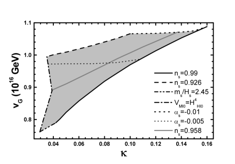
Figure 13: Allowed (lightly gray shaded) region in the $\kappa-v_{{}_{G}}$ plane for standard FHI followed by MI realized by a field which remains massless before MI. The conventions adopted for the various lines are also shown.

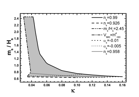
Figure 14: Allowed (lightly gray shaded) regions in the $\kappa-m_{s}/H_{s}$ plane for standard FHI followed by MI realized by a field which remains massless before MI. The conventions adopted for the various lines are also shown.

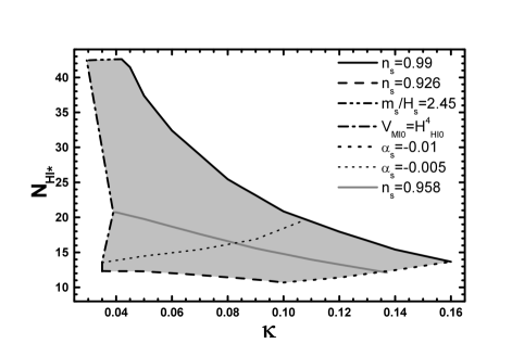
Figure 15: Allowed (lightly gray shaded) region in the $\kappa-N_{\rm HI*}$ plane for standard FHI followed by MI realized by a field which remains massless before MI. The conventions adopted for the various lines are also shown.

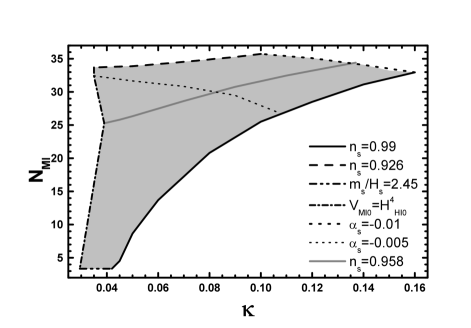
Figure 16: Allowed (lightly gray shaded) region in the $\kappa-N_{\rm MI}$ plane for standard FHI followed by MI realized by a field which remains massless before MI. The conventions adopted for the various lines are also shown.

• Standard FHI. We present the regions allowed by Eqs. (1), (19), (44), (47) – (50), (54) and (59) in the $\kappa-v_{{}_{G}}$ (Fig. 13), $\kappa-m_{s}/H_{s}$ (Fig. 14), $\kappa-N_{\rm HI*}$ (Fig. 15), and $\kappa-N_{\rm MI}$ (Fig. 16) plane. The conventions adopted for the various lines are displayed in the r.h.s of every graph. In particular, the black solid [dashed] lines correspond to $n_{\rm s}=0.99$ [$n_{\rm s}=0.926$] whereas the gray solid lines have been obtained by fixing $n_{\rm s}=0.958$ – see Eq. (1). The dot-dashed [double dot-dashed] lines correspond to the lower bound on $V_{\rm HI0}~{}[N_{\rm MI}]$ from Eq. (50) [Eq. (49)]. The bold [faint] dotted lines correspond to $\alpha_{\rm s}=-0.01$ [$\alpha_{\rm s}=-0.005$]. Let us notice that:

  • The resulting $v_{{}_{G}}$’s and $\kappa$’s are restricted to rather large values (although $v_{{}_{G}}<M_{\rm GUT}$) compared to those allowed within the other scenaria with one inflationary epoch (compare with Figs. 5 and 8). As a consequence, the SUGRA corrections in Eq. (10) play an important role.

  • The lower bound on $V_{\rm HI0}$ from Eq. (50) cut out sizeable slices of the allowed regions presented in Ref. [23]. This is due to the fact that we take here a much larger $m_{s}$ in order to fulfill Eq. (59) – not considered in Ref. [23].

  • The requirement of Eq. (47) does not constrain the parameters since it is overshadowed by the constraint of Eq. (50).

  • In almost the half of the available parameter space for $n_{\rm s}\sim 0.958$ we have relatively high $|\alpha_{\rm s}|$, $0.005\lesssim|\alpha_{\rm s}|\lesssim 0.01$.

  • For $n_{\rm s}=0.958$, we obtain $0.04\lesssim\kappa\lesssim 0.14$, $0.89\lesssim v_{{}_{G}}/(10^{16}~{}{\rm GeV})\lesssim 1.08$ and $0.003\lesssim|\alpha_{\rm s}|\lesssim 0.01$. Also, $12\lesssim N_{\rm HI*}\lesssim 21.7$, $35\gtrsim N_{\rm MI}\gtrsim 28$ and $0.64\lesssim m_{s}/H_{s}\lesssim 0.74$. So, the interesting solutions correspond to slow rather than fast-roll MI.

• Shifted FHI. We list input and output parameters consistent with Eqs. (19), (44), (47) – (50), (54) and (59) for the nearest to $M_{\rm GUT}$ $v_{{}_{G}}$ and selected $n_{\rm s}$’s in Table 4. The values of $v_{{}_{G}}$ come out considerably larger than in the case of standard FHI. However, the satisfaction of Eq. (50) in conjunction with Eq. (59) leads to $v_{{}_{G}}>M_{\rm GUT}$. Indeed, $v_{{}_{G}}=M_{\rm GUT}$ occurs for low $\kappa$’s which produce $V_{\rm HI0}$’s inconsistent with Eq. (50) – compare with Ref. [23].

• Smooth FHI. We arrange input and output parameters consistent with Eqs. (19), (44), (47) – (50), (54) and (59) for $v_{{}_{G}}=M_{\rm GUT}$ and selected $n_{\rm s}$’s in Table 4. In contrast with standard and shifted FHI, we can achieve $v_{{}_{G}}=M_{\rm GUT}$ for every $n_{\rm s}$ in the range of Eq. (1). The mSUGRA corrections in Eq. (10) play an important role for every $M_{\rm S}$ encountered in Table 4 and $|\alpha_{\rm s}|$ is considerably enhanced but compatible with Eq. (48).

  Shifted FHI				Smooth FHI
  $n_{\rm s}$	$0.926$	$0.958$	$0.99$	$n_{\rm s}$	$0.926$	$0.958$	$0.99$
  $v_{{}_{G}}/10^{16}~{}{\rm GeV}$	$5.86$	$6.4$	$6.91$	$v_{{}_{G}}/10^{16}~{}{\rm GeV}$	$2.86$	$2.86$	$2.86$
  $\kappa$	$0.035$	$0.04$	$0.045$	$M_{\rm S}/5\times 10^{17}~{}{\rm GeV}$	$0.815$	$0.87$	$0.912$
  $\sigma_{*}/10^{16}~{}{\rm GeV}$	$6.97$	$11.3$	$20.15$	$\sigma_{*}/10^{16}~{}{\rm GeV}$	$22.18$	$23.53$	$25.54$
  $M/10^{16}~{}{\rm GeV}$	$4.57$	$4.92$	$5.24$	$\mu_{\rm S}/10^{16}~{}{\rm GeV}$	$0.2$	$0.188$	$0.179$
  $1/\xi$	$4.2$	$4.13$	$4.09$	$\sigma_{\rm f}/10^{16}~{}{\rm GeV}$	$13.43$	$13.43$	$13.43$
  $N_{\rm HI*}$	$12.75$	$20.8$	$40.45$	$N_{\rm HI*}$	$13.6$	$18$	$26$
  $-\alpha_{\rm s}/10^{-3}$	$6$	$2.5$	$1$	$-\alpha_{\rm s}/10^{-3}$	$9$	$5.5$	$3$
  $N_{\rm MI}$	$31.1$	$23.1$	$3.35$	$N_{\rm MI}$	$30.3$	$25.6$	$17.8$
  $m_{s}/H_{s}$	$0.68$	$0.8$	$2.45$	$m_{s}/H_{s}$	$0.69$	$0.75$	$0.92$

  Table 4: Input and output parameters consistent with Eqs. (19), (44), (47) – (50), (54) and (59) in the cases of shifted ($M_{\rm S}=5\times 10^{17}~{}{\rm GeV}$) or smooth FHI for $s_{\rm Mi}/m_{\rm P}=0.01$, the nearest to $M_{\rm GUT}$ $v_{{}_{G}}$ and selected $n_{\rm s}$’s within the mSUGRA double inflationary scenario when the inflaton of MI does not acquire effective mass.

(ii)

If $s$ acquires mass, $s_{\rm Mi}$ can be evaluated from Eq. (53). However, due to our ignorance of $N_{\rm HI}$, there is an uncertainty in the determination of $m_{s}/H_{s}$, i.e. for every $N_{\rm MI}$ required by Eq. (44), we can derive a maximal [minimal], $m_{s}/H_{s}|_{\rm max}$ [$m_{s}/H_{s}|_{\rm min}$], value of $m_{s}/H_{s}$. Eq. (60) implies that $m_{s}/H_{s}|_{\rm max}$ [$m_{s}/H_{s}|_{\rm min}$] is obtained by using the minimal [maximal] possible value of $s_{\rm Mi}$ which corresponds to $N_{\rm HI}=N^{\rm max}_{\rm HI}$ [$N_{\rm HI}=N_{\rm HI*}$]. Our results are presented in Figs. 17 – 20 for standard FHI (with ${\sf N}=2$) and in Table 5 for shifted and smooth FHI. Let us discuss each case separately:

• Standard FHI. We present the regions allowed by Eqs. (1), (19), (44) and (47) – (49), (57) and (59) in the $\kappa-v_{{}_{G}}$ (Fig. 17), $\kappa-m_{s}/H_{s}$ (Fig. 18), $\kappa-N_{\rm HI*}$ (Fig. 19), and $\kappa-N_{\rm MI}$ (Fig. 20) plane. The conventions adopted for the various lines are displayed in the r.h.s of every graph. In particular, the black solid [dashed] lines correspond to $n_{\rm s}=0.99$ [$n_{\rm s}=0.926$] whereas the gray solid lines have been obtained by fixing $n_{\rm s}=0.958$ – see Eq. (1). The dot-dashed [double dot-dashed] lines correspond to the lower [upper] bound on $N_{\rm HI*}$ from Eq. (47) [Eq. (57)]. The double dot-dashed lines correspond to the upper [lower] bound on $m_{s}/H_{s}$ [$N_{\rm MI}$] from Eq. (36) [Eq. (49)]. The bold [faint] dotted lines correspond to $\alpha_{\rm s}=-0.01$ [$\alpha_{\rm s}=-0.005$]. Let us notice that:

  

  

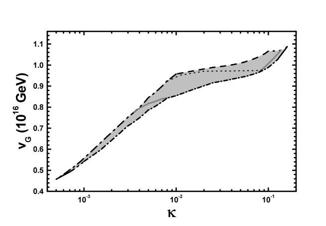
  Figure 17: Allowed (lightly gray shaded) region in the $\kappa-v_{{}_{G}}$ plane for standard FHI followed by MI realized by a field which acquires effective mass before MI. The conventions adopted for the various lines are also shown.

  

  

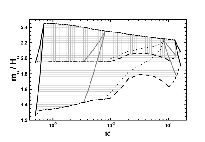
  Figure 18: Allowed regions in the $\kappa-m_{s}/H_{s}$ plane for $N_{\rm HI}=N_{\rm HI}^{\rm max}$ (dark gray ruled region) or $N_{\rm HI}=N_{\rm HI*}$ (lightly gray ruled region) and standard FHI followed by MI realized by a field which acquires effective mass before MI. The conventions adopted for the various lines are also shown.

  

  

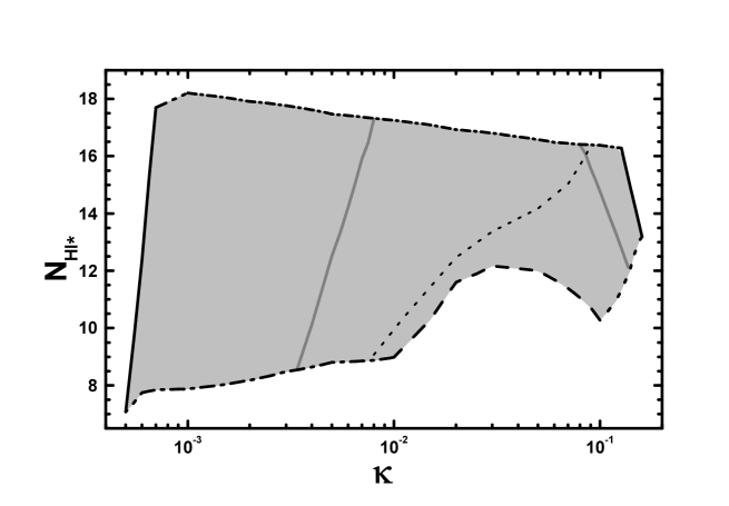
  Figure 19: Allowed (lightly gray shaded) region in the $\kappa-N_{\rm HI*}$ plane for standard FHI followed by MI realized by a field which acquires effective mass before MI. The conventions adopted for the various lines are also shown.

  

  

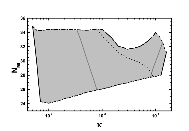
  Figure 20: Allowed (lightly gray shaded) region in the $\kappa-N_{\rm MI}$ plane for standard FHI followed by MI realized by a field which acquires effective mass before MI. The conventions adopted for the various lines are also shown.

  • Lower than those seen in Fig. 13 (but still larger than those shown in Figs. 5 and 8) $v_{{}_{G}}$’s and $\kappa$’s are allowed in Fig. 17, since the constraint of Eq. (50) is not applied here. As $\kappa$ increases above $0.01$ the mSUGRA corrections in Eq. (10) become more and more significant.

  • The constraint from the upper bound on $N_{\rm HI}$ in Eq. (57) is very restrictive and almost overshadows this from the lower bound on $N_{\rm MI}$ in Eq. (49) (which is applied, e.g., only in the upper left corner of the allowed region in Fig. 18).

  • In contrast with the case (i), $0.005\lesssim|\alpha_{\rm s}|\lesssim 0.01$ holds only in a very limited part of the allowed regions.

  • For $n_{\rm s}=0.958$, we obtain $0.0035\lesssim\kappa\lesssim 0.0085$ and $0.77\lesssim v_{{}_{G}}/(10^{16}~{}{\rm GeV})$ $\lesssim 0.85$, or $0.08\lesssim\kappa\lesssim 0.14$ and $0.96\lesssim v_{{}_{G}}/(10^{16}~{}{\rm GeV})\lesssim 1.08$. Also $0.002\lesssim|\alpha_{\rm s}|\lesssim 0.01$, $8.5\lesssim N_{\rm HI*}\lesssim 17.3$, $34.3\gtrsim N_{\rm MI}\gtrsim 26$ and $(1.4-1.96)\lesssim m_{s}/H_{s}\lesssim 2.35$. So, the interesting solutions correspond to fast rather than slow-roll MI.

  Shifted FHI				Smooth FHI
  $n_{\rm s}$	$0.926$	$0.958$	$0.99$	$n_{\rm s}$	$0.926$	$0.958$	$0.99$
  $v_{{}_{G}}/10^{16}~{}{\rm GeV}$	$2.86$	$1.93$	$12$	$v_{{}_{G}}/10^{16}~{}{\rm GeV}$	$2.86$	$3.3$	$4.61$
  $\kappa$	$0.0106$	$0.0055$	$0.13$	$M_{\rm S}/5\times 10^{17}~{}{\rm GeV}$	$0.815$	$1.06$	$1.66$
  $\sigma_{*}/10^{16}~{}{\rm GeV}$	$2.23$	$1.82$	$28.9$	$\sigma_{*}/10^{16}~{}{\rm GeV}$	$22.18$	$25.73$	$32.8$
  $M/10^{16}~{}{\rm GeV}$	$2.38$	$1.65$	$8.95$	$\mu_{\rm S}/10^{16}~{}{\rm GeV}$	$0.2$	$0.21$	$0.25$
  $1/\xi$	$4.67$	$5.04$	$4.05$	$\sigma_{\rm f}/10^{16}~{}{\rm GeV}$	$13.43$	$14.8$	$18.4$
  $N_{\rm HI*}$	$10.85$	$17.1$	$16.3$	$N_{\rm HI*}$	$13.6$	$16.6$	$16.5$
  $-\alpha_{\rm s}/10^{-3}$	$5.6$	$1.9$	$7.3$	$-\alpha_{\rm s}/10^{-3}$	$9$	$6.7$	$7.6$
  $N_{\rm MI}$	$32.6$	$26$	$28$	$N_{\rm MI}$	$30.3$	$27.4$	$27.6$
  $m_{s}/H_{s}|_{\rm max}$	$2.03$	$2.3$	$2.45$	$m_{s}/H_{s}|_{\rm max}$	$2.12$	$2.3$	$2.3$
  $m_{s}/H_{s}|_{\rm min}$	$1.6$	$2.3$	$2.45$	$m_{s}/H_{s}|_{\rm min}$	$1.94$	$2.3$	$2.3$

  Table 5: Input and output parameters consistent with Eqs. (19), (44) and (47) – (49), (57) and (59) in the cases of shifted ($M_{\rm S}=5\times 10^{17}~{}{\rm GeV}$) or smooth FHI for the nearest to $M_{\rm GUT}$ $v_{{}_{G}}$ and selected $n_{\rm s}$’s within the mSUGRA double inflationary scenario when the inflaton of MI acquires effective mass before MI.

• Shifted FHI. We list input and output parameters consistent with Eqs. (19), (44) and (47) – (49), (57) and (59) for the nearest to $M_{\rm GUT}$ $v_{{}_{G}}$ and selected $n_{\rm s}$’s in Table 5. The values of $v_{{}_{G}}$ come out again considerably larger than in the case of standard FHI. However, we take $v_{{}_{G}}=M_{\rm GUT}$ only for $n_{\rm s}=0.926$ since the satisfaction of Eq. (57) requires $v_{{}_{G}}<M_{\rm GUT}$ [$v_{{}_{G}}>M_{\rm GUT}$] for $n_{\rm s}=0.958$ [$n_{\rm s}=0.99$]. The closest to $M_{\rm GUT}$ values of $v_{{}_{G}}$ for $n_{\rm s}=0.958$ and $0.99$ are attained for $N_{\rm HI*}=N_{\rm HI}^{\rm max}$ and so, $m_{s}/H_{s}|_{\rm min}=m_{s}/H_{s}|_{\rm max}$.

• Smooth FHI. We display input and output parameters consistent with Eqs. (19), (44) and (47) – (49), (57) and (59) for the nearest to $M_{\rm GUT}$ $v_{{}_{G}}$ and selected $n_{\rm s}$’s in the Table 5. The results are quite similar to those for shifted FHI except for the fact that we have $v_{{}_{G}}>M_{\rm GUT}$ for $n_{\rm s}=0.958$ and $0.99$ and that $|\alpha_{\rm s}|$ remains considerably enhanced.

5 Conclusions

We reviewed the basic types (standard, shifted and smooth) of FHI in which the GUT breaking v.e.v, $v_{{}_{G}}$, turns out to be comparable to SUSY GUT scale, $M_{\rm GUT}$. Indeed, confronting these models with the restrictions on $P_{\cal R*}$ we obtain that $v_{{}_{G}}$ turns out a little lower than $M_{\rm GUT}$ for standard FHI whereas $v_{{}_{G}}=M_{\rm GUT}$ is possible for shifted and smooth FHI. However, the predicted $n_{\rm s}$ is just marginally consistent with the fitting of the WMAP3 data by the standard power-law $\Lambda$CDM cosmological model – if the horizon and flatness problems of SBB are resolved exclusively by FHI.

We showed that the results on $n_{\rm s}$ can be reconciled with data if we consider one of the following scenaria:

(i)

FHI within qSUGRA. In this case, acceptable $n_{\rm s}$’s can be obtained by appropriately restricting the parameter $c_{\rm q}$ involved in the quasi-canonical Kähler potential, with a convenient sign. We paid special attention to the monotonicity of the inflationary potential which is crucial for the safe realization of FHI. Enforcing the monotonicity constraint, reduction of $n_{\rm s}$ below around $0.95$ is prevented. Fixing in addition $n_{\rm s}$ to its central value, we found that (i) relatively large $\kappa$’s but rather low $v_{{}_{G}}$’s are required within standard FHI with $0.013\lesssim c_{\rm q}\lesssim 0.03$ and (ii) $v_{{}_{G}}=M_{\rm GUT}$ is possible within smooth FHI with $c_{\rm q}\simeq 0.0083$ but not within shifted FHI.

(ii)

FHI followed by MI. In this case, acceptable $n_{\rm s}$’s can be obtained by appropriately restricting the number of e-foldings $N_{\rm HI*}$. A residual number of e-foldings is produced by a bout of MI realized at an intermediate scale by a string modulus. We have taken into account extra restrictions on the parameters originating from:

• The resolution of the horizon and flatness problems of SBB.

• The requirements that FHI lasts long enough to generate the observed primordial fluctuations on all the cosmological scales and that these scales are not reprocessed by the subsequent MI.

• The limit on the running of $n_{\rm s}$.

• The naturalness of MI.

• The homogeneity of the present universe.

• The complete randomization of the modulus if this remains massless before MI or its evolution before MI if it acquires effective mass.

• The establishment of RD before the onset of NS.

We discriminated two basic versions of this scenario, depending whether the modulus does or does not acquire effective mass before MI. We concluded that:

• If the modulus remains massless before MI, the combination of the randomization and NS constraints pushes the values of the inflationary plateau to relatively large values. Fixing $n_{\rm s}$ to its central value, we got (i) $v_{{}_{G}}<M_{\rm GUT}$ and $10\lesssim N_{\rm HI*}\lesssim 21.7$ within the standard FHI, (ii) $v_{{}_{G}}>M_{\rm GUT}$ and $N_{\rm HI*}\simeq 21$ within shifted FHI and (iii) $v_{{}_{G}}=M_{\rm GUT}$ and $N_{\rm HI*}\simeq 18$ within smooth FHI. In all cases, MI of the slow-roll type, with $m_{s}/H_{s}\sim(0.6-0.8)$, and a mild (of the order of 0.01) tuning of the initial value of the modulus produces the necessary additional number of e-foldings.

• If the modulus acquires effective mass before MI, lower values, than those encountered in the case (i), of the inflationary plateau are available. Fixing $n_{\rm s}$ to its central value, we got (i) $v_{{}_{G}}<M_{\rm GUT}$ and $8.5\lesssim N_{\rm HI*}\lesssim 17.5$ within the standard FHI and (ii) $v_{{}_{G}}<M_{\rm GUT}$ [$v_{{}_{G}}>M_{\rm GUT}$] and $N_{\rm HI*}\simeq 17$ within shifted [smooth] FHI. In all cases, MI of the fast-roll type with $m_{s}/H_{s}\sim(1.4-2.45)$ and without any tuning of the initial value of the modulus produces the necessary additional number of e-foldings. However, FHI is constrained to be of short duration, producing a total number of e-foldings, $N_{\rm HI}\lesssim 17$. This is rather questionable and can be evaded by introducing a more elaborated structure for the Kähler potential or superpotential of the modulus (see, e.g., Ref. [35, 42]).

Trying to compare the proposed methods for the reduction of $n_{\rm s}$ within FHI, we can do the following comments:

• The main advantage of the method in the case (i) is that the standard one-step inflationary cosmological set-up remains intact. This method becomes rather attractive when the minimum-maximum structure of the inflationary potential is avoided. However, the possible in this way decrease of $n_{\rm s}$ is rather limited.

• The method of the case (ii) offers a comfortable reduction of $n_{\rm s}$ but it requires a more complicate cosmological set-up with advantages (dilution of gravitinos and defects) and disadvantages (complications with baryogenesis). The most natural and simple version of this scenario is realized when the modulus remains massless during FHI since it requires a very mild tuning.

Hopefully, the proposed scenaria will be further probed by the measurements of the Planck satellite which is expected to give results on $n_{\rm s}$ with an accuracy $\Delta n_{\rm s}\simeq 0.01$ by the end of the decade [47].

References

- [1]
- [2] A.H. Guth, Phys. Rev. D 23, 347 (1981).
- [3] D.H. Lyth and A. Riotto, Phys. Rept. 314, 1 (1999) [hep-ph/9807278].
-
[4]
G. Lazarides, Lect. Notes Phys. 592, 351 (2002)
[hep-ph/0111328];
G. Lazarides, J. Phys. Conf. Ser. 53, 528 (2006) [hep-ph/0607032]. - [5] A. Riotto, hep-ph/0210162.
- [6] G. Lazarides, hep-ph/0011130.
- [7] E.J. Copeland et al., Phys. Rev. D 49, 6410 (1994) [astro-ph/9401011].
-
[8]
G.R. Dvali, Q. Shafi and R.K. Schaefer, Phys. Rev. Lett.
73, 1886 (1994) [hep-ph/9406319];
G. Lazarides, R.K. Schaefer, and Q. Shafi, Phys. Rev. D 56, 1324 (1997) [hep-ph/9608256]. - [9] R. Jeannerot et al., J. High Energy Phys. 10, 012 (2000) [hep-ph/0002151].
-
[10]
G. Lazarides and C. Panagiotakopoulos,
Phys. Rev. D 52, 559 (1995) [hep-ph/9506325];
G. Lazarides et al., Phys. Rev. D 54, 1369 (1996) [hep-ph/9606297];
R. Jeannerot, S. Khalil, and G. Lazarides, Phys. Lett. B 506, 344 (2001) [hep-ph/0103229]. -
[11]
A.D. Linde and A. Riotto Phys. Rev. D 56, 1841 (1997) [hep-ph/9703209];
V.N. Şenoğuz and Q. Shafi, Phys. Lett. B 567, 79 (2003) [hep-ph/0305089]. -
[12]
D.N. Spergel et al., Astrophys. J.
Suppl. 170, 377 (2007) [astro-ph/0603449];
http://lambda.gsfc.nasa.gov/product/map/dr2/parameters.cfm. - [13] R.A. Battye et al., J. Cosmol. Astropart. Phys. 09, 007 (2006) [astro-ph/0607339].
- [14] G. Lazarides et al., Phys. Rev. D 70, 123527 (2005) [hep-ph/0409335].
- [15] R. Jeannerot and M. Postma, J. High Energy Phys. 05, 071 (2005) [hep-ph/0503146].
- [16] J. Rocher and M. Sakellariadou, J. Cosmol. Astropart. Phys. 03, 004 (2005) [hep-ph/0406120].
- [17] B. Garbrecht et al., J. High Energy Phys. 12, 038 (2006) [hep-ph/0605264].
- [18] M. Bastero-Gil, S.F. King, and Q. Shafi, Phys. Lett. B 651, 345 (2007) [hep-ph/0604198].
- [19] C. Panagiotakopoulos, Phys. Lett. B 402, 257 (1997) [hep-ph/9703443].
- [20] L. Boubekeur and D. Lyth, J. Cosmol. Astropart. Phys. 07, 010 (2005) [hep-ph/0502047].
- [21] M.ur Rehman, V.N. Şenoğuz, and Q. Shafi, Phys. Rev. D 75, 043522 (2007) [hep-ph/0612023].
- [22] G. Lazarides and A. Vamvasakis, arXiv:0705.3786.
-
[23]
G. Lazarides and C. Pallis, Phys. Lett. B 651, 216 (2006)
[hep-ph/0702260];
G. Lazarides, arXiv:0706.1436. -
[24]
P. Binétruy and M.K. Gaillard, Phys. Rev. D
34, 3069 (1986);
F.C. Adams et al., Phys. Rev. D 47, 426 (1993) [hep-ph/9207245];
T. Banks et al., Phys. Rev. D 52, 3548 (1995) [hep-ph/9503114];
R. Brustein et al., Phys. Rev. D 68, 023517 (2003) [hep-ph/0205042]. - [25] G. Lazarides and A. Vamvasakis, arXiv:0709.3362.
-
[26]
M. Dine, L. Randall and S. Thomas, Phys. Rev. Lett. 75, 398
(1995) [hep-ph/9503303];
M.K. Gaillard, H. Murayama and K.A. Olive, Phys. Lett. B 355, 71 (1995) [hep-ph/9504307]. - [27] D.H. Lyth and T. Moroi, J. High Energy Phys. 05, 004 (2004) [hep-ph/0402174].
- [28] A. Linde, J. High Energy Phys. 11, 052 (2001) [hep-ph/0110195].
- [29] G. Dvali, hep-ph/9503259.
-
[30]
M.Yu. Khlopov and A.D. Linde,
Phys. Lett. B 138, 265 (1984);
J. Ellis, J.E. Kim, and D.V. Nanopoulos, ibid. 145, 181 (1984). - [31] T.W.B. Kibble, J. Phys. A 9, 387 (1976).
- [32] G. Ballesteros et al., J. Cosmol. Astropart. Phys. 03, 001 (2006) [hep-ph/0601134].
- [33] V.N. Şenoğuz and Q. Shafi, Phys. Rev. D 71, 043514 (2005) [hep-ph/0412102].
-
[34]
D.H. Lyth and D. Wands,
Phys. Lett. B 524, 5 (2002) [hep-ph/0110002];
T. Moroi and T. Takahashi, Phys. Lett. B 522 215 (2001);
T. Moroi and T. Takahashi, Phys. Lett. B 539 303(E) (2002) [hep-ph/0110096];
D. H. Lyth, C. Ungarelli and D. Wands, Phys. Rev. D 67 023503 (2003) [astro-ph/0208055]. -
[35]
M. Kawasaki et al., Phys. Rev. D 68,
023508 (2003) [hep-ph/0304161];
M. Yamaguchi and J. Yokoyama, Phys. Rev. D 68, 123520 (2003) [hep-ph/0307373];
M. Yamaguchi and J. Yokoyama, Phys. Rev. D 70, 023513 (2004) [hep-ph/0402282];
M. Kawasaki et al., Phys. Rev. D 74, 043525 (2006) [hep-ph/0605271]. -
[36]
J. Garcia-Bellido et al., Phys. Rev. D 60, 123504 (1999) [hep-ph/9902449];
L.M. Krauss and M. Trodden, Phys. Rev. Lett. 83, 1502 (1999) [hep-ph/9902420]. - [37] K. Benakli and S. Davidson, Phys. Rev. D 60, 025004 (1999) [hep-ph/9810280].
- [38] G. Dvali and S. Kachru, hep-ph/0310244.
- [39] C.P. Burgess et al., J. High Energy Phys. 05, 067 (2005) [hep-th/0501125].
- [40] U. Seljak, et al., J. Cosmol. Astropart. Phys. 10, 014 (2006) [astro-ph/0604335].
-
[41]
A.A. Starobinsky and J. Yokoyama, Phys. Rev. D 50, 6357
(1994);
E.J. Chun, K. Dimopoulos and D. Lyth, Phys. Rev. D 70, 103510 (2004) [hep-ph/0402059]. -
[42]
K.I. Izawa, M. Kawasaki, and T. Yanagida, Phys. Lett. B 411, 249
(1997) [hep-ph/9707201];
M. Kawasaki, N. Sugiyama, and T. Yanagida, Phys. Rev. D 57, 6050 (1998) [hep-ph/9710259];
M. Kawasaki and T. Yanagida, Phys. Rev. D 59, 043512 (1999) [hep-ph/9807544]. -
[43]
G.D. Coughlan, W. Fischler, E. Kolb, S. Raby and G.G. Ross, Phys. Lett. B 131 (1983) 59;
B. de Carlos et al., Phys. Lett. B 318, 447 (1993) [hep-ph/9308325]. - [44] M. Berkooz, M. Dine and T. Volansky, Phys. Rev. D 71 103502 (2005) [hep-ph/0409226].
-
[45]
M. Endo et al., Phys. Rev. Lett.
96, 211301 (2006)
[hep-ph/0602061];
S. Nakamura and M. Yamaguchi, Phys. Lett. B 638, 389 (2006) [hep-ph/0602081]. - [46] C. Pallis, Nucl. Phys. B751, 129 (2006) [hep-ph/0510234].
- [47] http://www.rssd.esa.int/SA/PLANCK/include/report/redbook/redbook-science.htm