DESY-07-185

October 2007

A Momentum Space Analysis
of the Triple Pomeron Vertex in pQCD
J.  Bartels^(a) and K. Kutak^(b)

^(a)II. Institut für Theoretische Physik, Universität Hamburg
Luruper Chaussee 149, Germany
^(b) DESY Notkestrasse 85, 22607 Hamburg, Germany

()

We study properties of the momentum space Triple Pomeron Vertex in perturbative QCD. Particular attention is given to the collinear limit where transverse momenta on one side of the vertex are much larger than on the other side. We also comment on the kernels in nonlinear evolution equations.

1 Introduction

The Triple Pomeron Vertex (TPV) in perturbative QCD [1, 2, 3] has attracted significant attention in recent years. It is derived from the $2\to 4$ transition vertex in QCD reggeon field theory which represents the high energy description of QCD. In recent years particular interest has come from studies of nonlinear evolution equations, e.g. the Balitsky-Kovchegov equation [3, 4, 5], where the nonlinearity is given by the TPV. More recently, also generalizations of the nonlinear evolution have been considered [6] which contain pomeron loops [7]. Again, the TPV plays a central role in these investigations. Whereas in many studies and applications it is convenient to use the coordinate representation, it is important to understand the structure also in momentum space.

In this paper we will investigate some aspects of the TPV, starting from the momentum space representation of the $2\to 4$ gluon transition vertex, from which the TPV vertex has originally been derived [1, 2]. Many of the studies of the nonlinear evolution equations have been done in the context of deep inelastic scattering where a virtual photon scatters off a single nucleon or off a nucleus. In both cases the momentum scale of the photon is much larger that the typical scale of the hadron or nucleus, i.e. one is dealing with asymmetric momentum configurations. As a first step of investigating the TPV, therefore, we will focus on investigating the limit where the transverse momenta are strongly ordered. We also review and discuss the nonlinear evolution equation that have been proposed in the literature [8, 9], and we comment on the use of a twist-expansion in the low-$x$ limit.

The paper is organized as follows. In the following section 2 we define the setup of our calculation, and we construct the elastic amplitude for photon-photon scattering with exchange of a four gluon BKP state. In the large-$N_{c}$ limit, this reduces to photon-photon scattering with the exchange of a pomeron loop. In the remaining part of section 2 we define the Mellin transform of a pomeron loop and specify our use of ’collinear’ and ’anticollinear limits’. In section 3 we study the collinear limit of the Triple Pomeron Vertex in the large $N_{c}$ limit. Section 4 contains results of the analysis of the anticollinear limit in the large $N_{c}$ limit. In section 5 we extend the analysis to finite $N_{c}$. In section 6 we derive a hierarchy of nonlinear evolution equations which describe the interaction of a photon with a hadronic target. We also show that, in the mean field approximation, we obtain a nonlinear evolution equation for the unintegrated gluon density. Section 7 contains a few comments on the relation of this equation with other nonlinear evolution equations described in the literature. We end the paper with a few conclusions.

2 The $2\to 4$ gluon transition vertex

The LO momentum space expression for the $2\to 4$ gluon transition vertex has been derived in connection with the diffractive dissociation of the virtual photon in deep inelastic electron proton scattering [2].

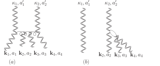
Figure 1: Examples of diagrams that contribute to the $2\to 4$ gluon transition vertex (wavy vertical lines represent reggeized gluons): (a) real emission, (b) a disconnected contribution.

More precisely, the process $\gamma^{*}+q\to(q\bar{q}+n\;\;gluons)+q$ has been investigated in the triple Regge limit. The resulting vertex consists of three pieces (we follow the notation of [11]):

$$\begin{split}{\cal V}^{a^{\prime}_{1}a^{\prime}_{2};a_{1}a_{2}a_{3}a_{4}}(\mbox{\boldmath{$\kappa$}}_{1},\mbox{\boldmath{$\kappa$}}_{2};\textbf{k}_{1},\textbf{k}_{2},\textbf{k}_{3},\textbf{k}_{4})=\frac{\sqrt{2}\pi\delta^{a^{\prime}_{1}a^{\prime}_{2}}}{N_{c}^{2}-1}\Bigg{[}\delta^{a_{1}a_{2}}\delta^{a_{3}a_{4}}V(\mbox{\boldmath{$\kappa$}}_{1},\mbox{\boldmath{$\kappa$}}_{2},\textbf{k}_{1},\textbf{k}_{2},\textbf{k}_{3},\textbf{k}_{4})\\ +\delta^{a_{1}a_{3}}\delta^{a_{2}a_{4}}V(\mbox{\boldmath{$\kappa$}}_{1},\mbox{\boldmath{$\kappa$}}_{2},\textbf{k}_{1},\textbf{k}_{3},\textbf{k}_{2},\textbf{k}_{4})+\delta^{a_{1}a_{4}}\delta^{a_{2}a_{3}}V(\mbox{\boldmath{$\kappa$}}_{1},\mbox{\boldmath{$\kappa$}}_{2},\textbf{k}_{1},\textbf{k}_{4},\textbf{k}_{2},\textbf{k}_{3})\Bigg{]},\end{split}$$ (1)

where $\mbox{\boldmath{$\kappa$}}_{1}+\mbox{\boldmath{$\kappa$}}_{2}=\textbf{k}_{1}+\textbf{k}_{2}+\textbf{k}_{3}+\textbf{k}_{4}=\textbf{q}$, and the subscripts $a_{i}^{\prime}$, $a_{i}$ refer to the color degrees of freedom of the reggeized gluons. It is convenient to express the ’basic vertex function’ $V(\mbox{\boldmath{$\kappa$}}_{1},\mbox{\boldmath{$\kappa$}}_{2},\textbf{k}_{1},\textbf{k}_{2},\textbf{k}_{3},\textbf{k}_{4})$ in terms of another function $G(\mbox{\boldmath{$\kappa$}}_{1},\mbox{\boldmath{$\kappa$}}_{2},\textbf{k}_{1},\textbf{k}_{2},\textbf{k}_{3})$:

$$\begin{split}V(\mbox{\boldmath{$\kappa$}}_{1},\mbox{\boldmath{$\kappa$}}_{2},\textbf{k}_{1},\textbf{k}_{2},\textbf{k}_{3},\textbf{k}_{4})=\frac{1}{2}g^{4}\bigg{[}G(\mbox{\boldmath{$\kappa$}}_{1},\mbox{\boldmath{$\kappa$}}_{2},\textbf{k}_{1},\textbf{k}_{2}+\textbf{k}_{3},\textbf{k}_{4})+G(\mbox{\boldmath{$\kappa$}}_{1},\mbox{\boldmath{$\kappa$}}_{2},\textbf{k}_{2},\textbf{k}_{1}+\textbf{k}_{3},\textbf{k}_{4})\\ +G(\mbox{\boldmath{$\kappa$}}_{1},\mbox{\boldmath{$\kappa$}}_{2},\textbf{k}_{1},\textbf{k}_{2}+\textbf{k}_{4},\textbf{k}_{3})+G(\mbox{\boldmath{$\kappa$}}_{1},\mbox{\boldmath{$\kappa$}}_{2},\textbf{k}_{2},\textbf{k}_{1}+\textbf{k}_{4},\textbf{k}_{3})-G(\mbox{\boldmath{$\kappa$}}_{1},\mbox{\boldmath{$\kappa$}}_{2},\textbf{k}_{1}+\textbf{k}_{2},\textbf{k}_{3},\textbf{k}_{4})\\ -G(\mbox{\boldmath{$\kappa$}}_{1},\mbox{\boldmath{$\kappa$}}_{2},\textbf{k}_{1}+\textbf{k}_{2},\textbf{k}_{4},\textbf{k}_{3})-G(\mbox{\boldmath{$\kappa$}}_{1},\mbox{\boldmath{$\kappa$}}_{2},\textbf{k}_{1},\textbf{k}_{2},\textbf{k}_{3}+\textbf{k}_{4})-G(\mbox{\boldmath{$\kappa$}}_{1},\mbox{\boldmath{$\kappa$}}_{2},\textbf{k}_{2},\textbf{k}_{1},\textbf{k}_{3}+\textbf{k}_{4})\\ +G(\mbox{\boldmath{$\kappa$}}_{1},\mbox{\boldmath{$\kappa$}}_{2},\textbf{k}_{1}+\textbf{k}_{2},-,\textbf{k}_{3}+\textbf{k}_{4})\bigg{]}.\end{split}$$ (2)

This function $G(\mbox{\boldmath{$\kappa$}}_{1},\mbox{\boldmath{$\kappa$}}_{2},\textbf{k}_{1},\textbf{k}_{2},\textbf{k}_{3})$ [13, 16] generalizes the $G$ function introduced in [2] to the non-forward direction. This function can again be split into two pieces:

$$G(\mbox{\boldmath{$\kappa$}}_{1},\mbox{\boldmath{$\kappa$}}_{2},\textbf{k}_{1},\textbf{k}_{2},\textbf{k}_{3})=G_{1}(\mbox{\boldmath{$\kappa$}}_{1},\mbox{\boldmath{$\kappa$}}_{2},\textbf{k}_{1},\textbf{k}_{2},\textbf{k}_{3})+G_{2}(\mbox{\boldmath{$\kappa$}}_{1},\mbox{\boldmath{$\kappa$}}_{2},\textbf{k}_{1},\textbf{k}_{2},\textbf{k}_{3}),$$ (3)

where the first part contains the ’connected contributions’ (also: ’real contributions’):

$$G_{1}(\mbox{\boldmath{$\kappa$}}_{1},\mbox{\boldmath{$\kappa$}}_{2},\textbf{k}_{1},\textbf{k}_{2},\textbf{k}_{3})=\frac{(\textbf{k}_{2}+\textbf{k}_{3})^{2}\mbox{\boldmath{$\kappa$}}_{1}^{2}}{(\mbox{\boldmath{$\kappa$}}_{1}-\textbf{k}_{1})^{2}}+\frac{(\textbf{k}_{1}+\textbf{k}_{2})^{2}\mbox{\boldmath{$\kappa$}}_{2}^{2}}{(\mbox{\boldmath{$\kappa$}}_{2}-\textbf{k}_{3})^{2}}-\frac{\textbf{k}_{2}^{2}\mbox{\boldmath{$\kappa$}}_{1}^{2}\mbox{\boldmath{$\kappa$}}_{2}^{2}}{(\mbox{\boldmath{$\kappa$}}_{1}-\textbf{k}_{1})^{2}(\mbox{\boldmath{$\kappa$}}_{2}-\textbf{k}_{3})^{2}}$$

$$-(\textbf{k}_{1}+\textbf{k}_{2}+\textbf{k}_{3})^{2},$$ (4)

and the second one takes care of the disconnected (’virtual’) pieces:

$$g^{2}G_{2}(\mbox{\boldmath{$\kappa$}}_{1},\mbox{\boldmath{$\kappa$}}_{2},\textbf{k}_{1},\textbf{k}_{2},\textbf{k}_{3}) = -\frac{\mbox{\boldmath{$\kappa$}}_{1}^{2}\mbox{\boldmath{$\kappa$}}_{2}^{2}}{N_{c}}\Big{(}[\omega(\textbf{k}_{2})-\omega(\textbf{k}_{2}+\textbf{k}_{3})]\delta^{(2)}(\mbox{\boldmath{$\kappa$}}_{1}-\textbf{k}_{1})$$ (5)

$$+[\omega(\textbf{k}_{2})-\omega(\textbf{k}_{1}+\textbf{k}_{2})]\delta^{(2)}(\mbox{\boldmath{$\kappa$}}_{1}-\textbf{k}_{1}-\textbf{k}_{2})\Big{)}.$$

Here $\omega(\textbf{k})$ denotes the trajectory function.:

$$\omega(\textbf{k})=-N_{c}g^{2}\int\frac{d^{2}\textbf{l}}{(2\pi)^{3}}\frac{\textbf{k}^{2}}{\textbf{l}^{2}+(\textbf{k}-\textbf{l})^{2}}\frac{1}{(\textbf{k}-\textbf{l})^{2}}.$$ (6)

The vertex (1) is completely symmetric under the permutation of the four gluons. It is infrared finite, it has been shown to be invariant under Möbius transformations  [12], and it vanishes when $\mbox{\boldmath{$\kappa$}}_{i}$ or $\textbf{k}_{i}$ goes to zero.

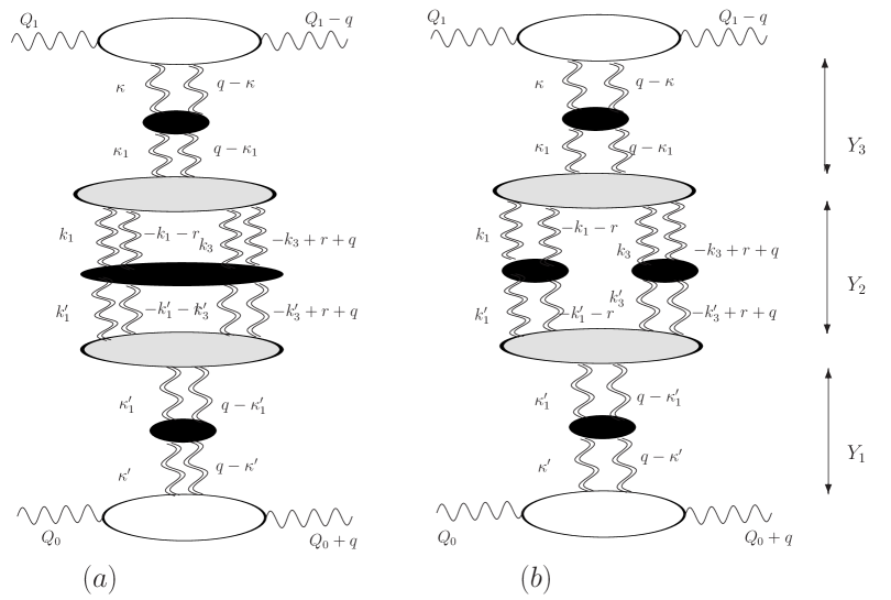
Figure 2: Contributions to the elastic scattering of two virtual photons which contain the $2\to 4$ gluon vertex (dark blobs represent Green’s functions of reggeized gluons): (a) the four gluon BKP state; (b) a Pomeron loop.

This vertex can be used to construct, in reggeon field theory, the selfenergy $\Sigma$, of the BFKL Green’s function (Fig. 2). In the lowest order contribution to $\Sigma$, we have a BKP state between two $2\to 4$ vertices, which contains all pairwise interactions of four reggeized $t$-channel gluons. Its Green’s function satisfies the following evolution equation:

$$(\omega-\omega(\textbf{k}_{1})-\omega(\textbf{k}_{2})-\omega(\textbf{k}_{3})-\omega(\textbf{k}_{4})){\cal G}^{(4)\;\{a_{i}\},\{a^{\prime}_{i}\}}_{\omega}(\{\textbf{k}_{i}\},\{\textbf{k}^{\prime}_{i}\})=$$

$${\cal G}^{(4)0\;\{a_{i}\},\{a^{\prime}_{i}\}}(\{\textbf{k}_{i}\},\{\textbf{k}^{\prime}_{i}\})\;+\;\sum_{(ij)}\frac{1}{\textbf{k}_{i}^{2}\textbf{k}_{j}^{2}}K_{2\rightarrow 2}^{\{a\}\rightarrow\{b\}}\,\otimes\,{\cal G}^{(4)\;\{b_{i}\}\{a^{\prime}_{i}\}}_{\omega}(\{\textbf{k}_{i}\}\{\textbf{k}^{\prime}_{i}\}),$$ (7)

where we have used the shorthand notation $\{\textbf{k}_{i}\}=(\textbf{k}_{1},\textbf{k}_{2},\textbf{k}_{3},\textbf{k}_{4})$ etc. The sum extends over all pairs $(ij)$ of gluons, the kernel $K_{2\rightarrow 2}^{\{a\}\rightarrow\{b\}}$ includes the color tensor $f_{a_{i}b_{i}c}f_{a_{j}b_{j}c}$

$$K_{2\rightarrow 2}^{\{a_{i}\}\rightarrow\{b_{i}\}}=g^{2}\;f_{b_{1}a_{1}c}f_{ca_{2}b_{2}}\left[\textbf{r}^{2}-\frac{\textbf{k}_{1}^{2}(\textbf{k}-\textbf{r})^{2}}{(\textbf{k}_{1}-\textbf{k})^{2}}-\frac{\textbf{k}^{2}(\textbf{k}_{1}-\textbf{r})^{2}}{(\textbf{k}_{1}-\textbf{k})^{2}}\right],\\$$ (8)

and the convolution symbol $\otimes$ stands for $\int\!\!\frac{d\textbf{k}^{2}}{(2\pi)^{3}}$. The inhomogeneous term has the form:

$$\delta^{(2)}(\sum\textbf{k}_{i}-\sum\textbf{k}_{i}^{\prime}){\cal G}^{(4)0\;\{a_{i}\}\{a^{\prime}_{i}\}}(\{\textbf{k}_{i}\},\{\textbf{k}^{\prime}_{i}\})=(2\pi)^{9}\prod_{1}^{4}\frac{\delta_{a_{i}a^{\prime}_{i}}\delta^{(2)}(\textbf{k}_{i}-\textbf{k}^{\prime}_{i})}{\textbf{k}_{i}^{2}}.$$ (9)

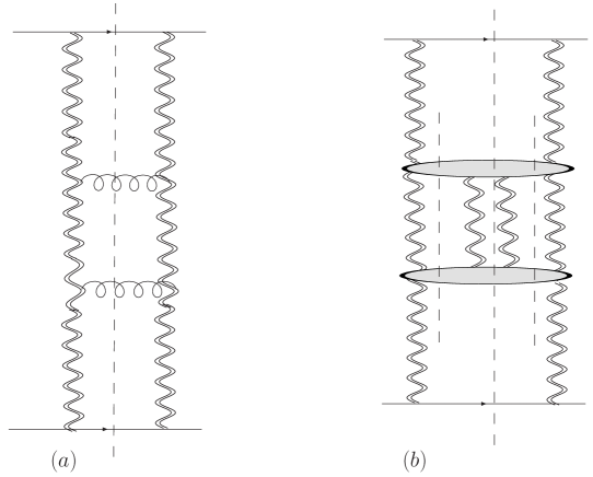
Figure 3: Quark quark scattering in the high energy limit of QCD (color singlet exchange): (a) two loop correction in the ladder approximation, (b) diagrams with two Triple Pomeron Vertices (grey bloobs).

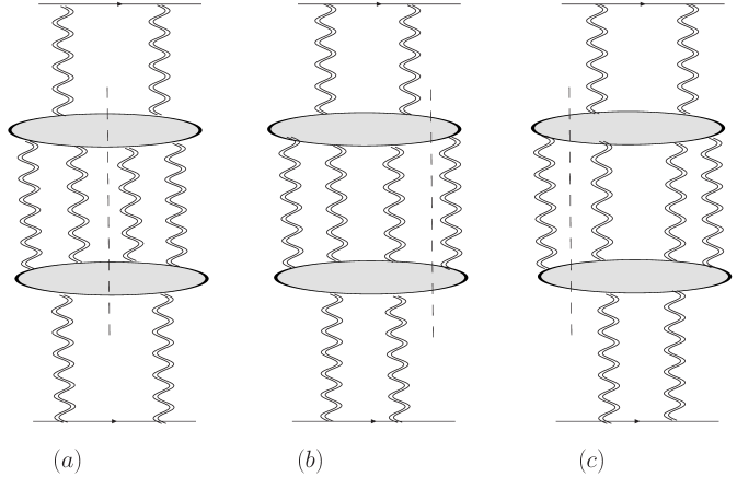
Figure 4: Different cuts.

Let us briefly explain how we obtain the correct normalization factors. We consider the scattering amplitude of quark quark scattering (Fig.3b) which, in the center, contains the insertion of four reggeized $t$-channel gluons. We begin with the diffractive cut (Fig.4a): the one loop amplitude on the lhs of the cutting line will be assumed to have an even signature exchange and, hence, is equal (up to factor $i$) to its energy disconinuity. As a result, we start from Fig. 3b with three cutting lines: all horizontal lines are on mass-shell. To distribute the color and phase space factors we proceed as follows: using the on-shell conditions, we can perform $8$ out of the $10$ longitudinal Sudakov integrations; the two remaining longitudinal variables denote the rapidity of the two produced gluons in the central region which, for the moment, we keep fixed. For each closed loop, we are left with an integral $\int d^{2}k/(2\pi)^{3}$. For each BFKL rung in Fig.3a we have the kernel from (8), for each $2\to 4$ vertex in Fig.3b we have the $2\to 4$ vertex (1) (divided by the additional factor $1/\sqrt{2}$). Having in mind that our discussion should be applicable also to more general diagrams, we retain, for the moment, the general color structure in (8) and in (1). When deriving, from Fig.3b, the diffractive cut in Fig.4a, we write, for each $2$ gluon exchange on the lhs and on the rhs of the cutting line a statistic factor $1/2!$; from the compensating factor $4$ we absorb $\sqrt{2}$ into each of the $2\to 4$ vertices. As a result, we have, in addition to all other color and phase space factors, the statistic factors $2/(2!)^{2}$. Invoking now the AGK rules  [14, 15], applied to the exchange of four (odd signature) reggeized gluons, the other contributions in Figs.4b and c, the statistic factors become:

$$2\left(\frac{1}{2!2!}-\frac{2}{3!}\right)=-\frac{4}{4!}.$$ (10)

Finally, we use our result for quark-quark scattering and return to the process of our interest, photon-photon scattering. Replacing the quark impact factors by photon impact factors, inserting BFKL rungs above and below the $2\to 4$ vertices, and inserting pairwise interactions between the four gluon lines in the center, we arrive at:

$$A(s,t) = 2is\pi\int_{0}^{Y}dY_{3}\int_{0}^{Y}dY_{2}\int_{0}^{Y}dY_{1}\delta(Y-Y_{1}-Y_{2}-Y_{3})$$ (11)

$$\cdot\int\frac{d^{2}\mbox{\boldmath{$\kappa$}}}{(2\pi)^{3}}\frac{d^{2}\mbox{\boldmath{$\kappa$}}_{1}}{(2\pi)^{3}}\phi^{a^{\prime}_{1}a^{\prime}_{2}}(\mbox{\boldmath{$\kappa$}},\textbf{q}-\mbox{\boldmath{$\kappa$}}){\cal G}^{(2)a_{1}^{\prime}a_{2}^{\prime};a_{1}^{\prime\prime}a_{2}^{\prime\prime}}(Y_{3};\mbox{\boldmath{$\kappa$}},\mbox{\boldmath{$\kappa$}}_{1},\textbf{q})$$

$$\cdot\frac{-4}{4!}\int\prod_{i=1}^{4}\left(\frac{d^{2}k_{i}}{(2\pi)^{3}}\right)(2\pi)^{3}\delta^{(2)}(\sum\textbf{k}_{i}-\textbf{q})\int\prod_{i=1}^{4}\left(\frac{d^{2}\textbf{k}_{i}^{\prime}}{(2\pi)^{3}}\right)(2\pi)^{3}\delta^{(2)}(\sum\textbf{k}_{i}^{\prime}-\textbf{q})$$

$$\cdot{\cal V}^{a_{1}^{\prime\prime}a_{2}^{\prime\prime};a_{1}a_{2}a_{3}a_{4}}(\mbox{\boldmath{$\kappa$}}_{1},\textbf{q}-\mbox{\boldmath{$\kappa$}}_{1};\textbf{k}_{1},\textbf{k}_{2},\textbf{k}_{3},\textbf{k}_{4}){\cal G}^{(4);\{a_{i}\}\{b_{i}\}}(Y_{2};\{\textbf{k}_{i}\}\{\textbf{k}_{i}^{\prime}\})$$

$$\cdot\int\frac{d^{2}\mbox{\boldmath{$\kappa$}}^{\prime}}{(2\pi)^{3}}\frac{d^{2}\mbox{\boldmath{$\kappa$}}_{1}^{\prime}}{(2\pi)^{3}}{\cal V}^{b_{1}b_{2}b_{3}b_{4};b_{1}^{\prime\prime}b_{2}^{\prime\prime}}(\textbf{k}_{1}^{\prime},\textbf{k}_{2}^{\prime},\textbf{k}_{3}^{\prime},\textbf{k}_{4}^{\prime};\mbox{\boldmath{$\kappa$}}^{\prime}_{1},\textbf{q}-\mbox{\boldmath{$\kappa$}}^{\prime}_{1})$$

$$\cdot{\cal G}^{(2)b_{1}^{\prime\prime}b_{2}^{\prime\prime},b_{1}^{\prime}b_{2}^{\prime}}(Y_{1};\mbox{\boldmath{$\kappa$}}^{\prime}_{1},\mbox{\boldmath{$\kappa$}}^{\prime},\textbf{q})\phi^{b^{\prime}_{1}b^{\prime}_{2}}(\mbox{\boldmath{$\kappa$}}^{\prime},\textbf{q}-\mbox{\boldmath{$\kappa$}}^{\prime}),$$

where the minus sign in the third line indicates that the four gluon insertion into the two gluon Green’s function represents a negative correction to the simple ladder amplitude. Here $s$ is the squared center of mass energy, $Y\!\!=\!\ln(s/s_{0})$ is the total rapidity, $Y_{1}$, $Y_{2}$, $Y_{3}$ are the rapidity intervals as depicted in Fig. 2, $\phi^{a^{\prime}_{1}a^{\prime}_{2}}$ denotes the impact factor of the virtual photon, ${\cal G}^{(2)a_{1}^{\prime}a_{2}^{\prime};a_{1}^{\prime\prime}a_{2}^{\prime\prime}}_{\omega}$ is the BFKL Green’s function which satisfies the BFKL integral equation:

$$(\omega-\omega(\textbf{k}_{1})-\omega(\textbf{k}_{2})){\cal G}^{(2)\;a_{1}a_{2}b_{1}b_{2}}_{\omega}(\{\textbf{k}_{i}\},\{\textbf{k}^{\prime}_{i}\})=$$

$${\cal G}^{(2)0\;a_{1}a_{2}b_{1}b_{2}}(\{\textbf{k}_{i}\},\{\textbf{k}^{\prime}_{i}\})\;+\;\frac{1}{\textbf{k}_{1}^{2}\textbf{k}_{2}^{2}}K_{2\rightarrow 2}^{\{a\}\rightarrow\{b\}}\,\otimes\,{\cal G}^{(2)\;a_{1}a_{2}b_{1}b_{2}}_{\omega}(\{\textbf{k}_{i}\}\{\textbf{k}^{\prime}_{i}\}),$$ (12)

with an inhomogeneous term analogous to (9). The statistics factor $\frac{1}{4!}$ reflects the symmetry of the expression under the interchange of the four gluons. In eq.(11), the selfenergy is defined by lines 3 - 5, i.e. the convolution of the two $2\to 4$ vertices with the BKP Green’s function between them. As a convenient simplification, we approximate the four gluon state by two noninteracting color singlet ladders (Fig. 2b): this configuration represents a ’pomeron loop’. It is easy to find the combinatorial factor of a system where two pairs of gluons form bound states. We have three possibilities of pairing two gluons to form bound states out of four gluons. This yields the factor $1/2!$. In this configuration we have a pomeron loop topology. The result reads:

$$A(s,t)=2is\pi\int_{0}^{Y}dY_{3}\int_{0}^{Y}dY_{2}\int_{0}^{Y}dY_{1}\;\delta(Y-Y_{1}-Y_{2}-Y_{3})$$

$$\cdot\int\!\!\!\frac{d^{2}\mbox{\boldmath{$\kappa$}}}{(2\pi)^{3}}\frac{d^{2}\mbox{\boldmath{$\kappa$}}_{1}}{(2\pi)^{3}}\phi^{a^{\prime}_{1}a^{\prime}_{2}}(\mbox{\boldmath{$\kappa$}},\textbf{q}-\mbox{\boldmath{$\kappa$}}){\cal G}^{(2)a_{1}^{\prime}a_{2}^{\prime},a_{1}^{{}^{\prime\prime}}a_{2}^{{}^{\prime\prime}}}(Y_{3};\mbox{\boldmath{$\kappa$}},\mbox{\boldmath{$\kappa$}}_{1},\textbf{q})$$

$$\cdot\frac{-1}{2!}\int\frac{d^{2}\textbf{r}}{(2\pi)^{3}}\int\frac{d^{2}\textbf{k}_{1}}{(2\pi)^{3}}\frac{d^{2}\textbf{k}_{3}}{(2\pi)^{3}}{\cal V}^{a_{1}^{\prime\prime}a_{2}^{\prime\prime};a_{1}a_{2}a_{3}a_{4}}(\mbox{\boldmath{$\kappa$}}_{1},\textbf{q}-\mbox{\boldmath{$\kappa$}}_{1};\textbf{k}_{1},-\textbf{k}_{1}-\textbf{r},\textbf{k}_{3},-\textbf{k}_{3}+\textbf{r}+\textbf{q})$$

$$\cdot\int\frac{d^{2}\textbf{k}_{1}^{\prime}}{(2\pi)^{3}}\frac{d^{2}\textbf{k}_{3}^{\prime}}{(2\pi)^{3}}(P{\cal G})^{(2)a_{1}a_{2}b_{1}b_{2}}(Y_{2};\textbf{k}_{1},\textbf{k}_{1}^{\prime},\textbf{r})(P{\cal G})^{(2)a_{3}a_{4}b_{3}b_{4}}(Y_{2};\textbf{k}_{3},\textbf{k}_{3}^{\prime},\textbf{r}+\textbf{q})$$

$$\cdot\int\frac{d^{2}\mbox{\boldmath{$\kappa$}}^{\prime}_{1}}{(2\pi)^{3}}\frac{d^{2}\mbox{\boldmath{$\kappa$}}^{\prime}}{(2\pi)^{3}}{\cal V}^{b_{1}b_{2}b_{3}b_{4};b_{1}^{\prime\prime}b_{2}^{\prime\prime}}(\textbf{k}_{1}^{\prime},-\textbf{k}_{1}^{\prime}-\textbf{r},\textbf{k}_{3}^{\prime},-\textbf{k}_{3}^{\prime}+\textbf{r}+\textbf{q};\mbox{\boldmath{$\kappa$}}_{1}^{\prime},\textbf{q}-\mbox{\boldmath{$\kappa$}}_{1}^{\prime})$$

$$\cdot{\cal G}^{(2)b_{1}^{\prime\prime}b_{2}^{\prime\prime},b^{\prime}_{1}b^{\prime}_{2}}(Y_{1};\mbox{\boldmath{$\kappa$}}_{1}^{\prime},\mbox{\boldmath{$\kappa$}}^{\prime},\textbf{q})\phi^{b^{\prime}_{1}b^{\prime}_{2}}(\mbox{\boldmath{$\kappa$}}^{\prime},\textbf{q}-\mbox{\boldmath{$\kappa$}}^{\prime}),$$ (13)

where

$$P^{a_{1}a_{2}b_{1}b_{2}}=\frac{\delta^{a_{1}a_{2}}\delta^{b_{1}b_{2}}}{N_{c}^{2}-1}$$ (14)

is the color singlet projector. These projectors act on the color tensors of the $2\to 4$ vertices, turning the pairs of color labels $(a_{1}a_{2})$, $(b_{1}b_{2})$, $(a_{3}a_{4})$, $(b_{3}b_{4})$ into color singlets. Comparison with (1) shows that this projection operator, when acting on the first term, leads to a factor $1$, whereas the remaining terms come with the weight factor $\frac{1}{N^{2}-1}$: in comparison with the first term, they are color suppressed. This large-$N_{c}$ approximation turns the $2\to 4$ vertices into the Triple Pomeron Vertices (TVP).

In the following we shall focus on the pomeron loop (13) and investigate, for zero total momentum transfer, $\textbf{q}=0$, the kinematic limit where the momentum scale of the upper photon is much larger than the lower one. This implies that, at the upper TPV, the momentum from above, $\mbox{\boldmath{$\kappa$}}_{1}$, is larger than the momenta from below, $\textbf{k}_{1}$, $\textbf{k}_{3}$, and the loop momentum r (’collinear limit’). Conversely, for the lower TPV we have the opposite situation: the momenta $\textbf{k}_{1}^{\prime}$, $\textbf{k}_{3}^{\prime}$, and r are larger than $\mbox{\boldmath{$\kappa$}}_{1}^{\prime}$ (’anticollinear limit’). Let us become a bit more formal. We expand the amplitude of Fig. 2 in powers of $Q_{0}^{2}/Q_{1}^{2}$ (’twist expansion’). The object of our interest is the self-energy of the Pomeron Green’s function, $\Sigma(\mbox{\boldmath{$\kappa$}}_{1},\mbox{\boldmath{$\kappa$}}^{\prime}_{1})$. In Eq.(13), $\Sigma(\mbox{\boldmath{$\kappa$}}_{1},\mbox{\boldmath{$\kappa$}}^{\prime}_{1})$ is defined to represent the lines 3 - 5, i.e. the convolution of the two TPV’s with the two BFKL Green functions between them. It has the dimension $\textbf{k}^{2}$, and it is convenient to define the dimensionless object $\tilde{\Sigma}(\frac{\mbox{\boldmath{$\kappa$}}_{1}}{\mbox{\boldmath{$\kappa$}}^{\prime}_{1}})=\frac{\Sigma(\mbox{\boldmath{$\kappa$}}_{1},\mbox{\boldmath{$\kappa$}}^{\prime}_{1})}{\sqrt{\mbox{\boldmath{$\kappa$}}_{1}^{2}\mbox{\boldmath{$\kappa$}}_{1}^{{}^{\prime}2}}}$ with the Mellin transform:

$$\tilde{\Sigma}(\gamma)=\int_{0}^{\infty}dk^{2}\tilde{\Sigma}(k^{2})(k^{2})^{\gamma-1}.$$ (15)

The inverse Mellin transform reads:

$$\tilde{\Sigma}(k^{2})=\int_{C}\frac{d\gamma}{2\pi i}(k^{2})^{-\gamma}\tilde{\Sigma}(\gamma),$$ (16)

where $k^{2}=\frac{\mbox{\boldmath{$\kappa$}}_{1}^{{}^{\prime}2}}{\mbox{\boldmath{$\kappa$}}_{1}^{2}}$, and the contour crosses the real axis between $-1$ and $0$ (see Fig. 5). Our analysis will then reduce to the study of the singularities of the function $\tilde{\Sigma}(\gamma)$. The twist expansion corresponds to the analysis of the poles located to the left of the contour in the $\gamma$ plane: the pole at $\gamma=-1$ is the leading twist pole, the pole at $\gamma=-2$ belongs to twist 4, and so on. As we have already said before, for the upper TPV in Fig. 2, the analysis of this twist expansion requires the ’collinear limit’, for the lower TVP the ’anticollinear’ one.

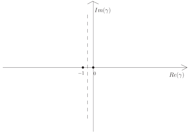
Figure 5: Singularities in the $\gamma$ plane.

3 The collinear limit

In this section we are going to study the collinear limit of the TPV. The ordering of the transverse momenta is the following: $|\mbox{\boldmath{$\kappa$}}_{1}|\equiv|\textbf{k}|\!\!\gg\!\!|\textbf{k}_{1}|,|\textbf{k}_{2}|,|\textbf{k}_{3}|,|\textbf{k}_{4}|$. We therefore expand in powers of $|\textbf{k}_{1}|/|\textbf{k}|$, $|\textbf{k}_{2}|/|\textbf{k}|$, $|\textbf{k}_{3}|/|\textbf{k}|$, $|\textbf{k}_{4}|/|\textbf{k}|$. In our investigations we will be interested in attaching color singlet objects to the vertex, and we project (1) onto the color singlets. In the limit $N_{c}\to\infty$ we obtain:

$$P^{a_{1}a_{2}b_{1}b_{2}}P^{a_{3}a_{4}b_{3}b_{4}}{\cal V}^{a^{\prime}_{1}a^{\prime}_{2};a_{1}a_{2}a_{3}a_{4}}(\textbf{k},-\textbf{k};\textbf{k}_{1},\textbf{k}_{2},\textbf{k}_{3},\textbf{k}_{4})=$$

$$= \delta^{a_{1}^{\prime},a_{2}^{\prime}}\delta^{b_{1},b_{2}}\delta^{b_{3},b_{4}}\frac{\sqrt{2}\pi}{N_{c}^{2}-1}\bigg{[}V(1,2,3,4)+\frac{1}{N^{2}-1}\left(V(1,3,2,4)+V(1,4,2,3)\right)\bigg{]},$$ (17)

where $V(1,2,3,4)\equiv V(\textbf{k},-\textbf{k};\textbf{k}_{1},\textbf{k}_{2},\textbf{k}_{3},\textbf{k}_{4})$. The first term will be denoted by

$${\cal V}_{L0N_{c}}^{\{a^{\prime}\}\{b\}}(1,2,3,4)=\delta^{a_{1}^{\prime},a_{2}^{\prime}}\delta^{b_{1},b_{2}}\delta^{b_{3},b_{4}}\frac{\sqrt{2}\pi}{N_{c}^{2}-1}V(1,2,3,4),$$ (18)

the second and third ones by

$${\cal V}_{subN_{c}}^{\{a^{\prime}\}\{b\}}(1,3,2,4)=\delta^{a_{1}^{\prime},a_{2}^{\prime}}\delta^{b_{1},b_{2}}\delta^{b_{3},b_{4}}\frac{\sqrt{2}\pi}{(N_{c}^{2}-1)^{2}}V(1,3,2,4)$$ (19)

etc.

3.1 The real part

Let us begin the analysis by expanding the real part of the $G$ function (3) in the collinear limit. As we are going to limit ourselves to the forward case we use the simplified notations $G(\textbf{k},-\textbf{k};\textbf{k}_{1},-\textbf{k}_{1}-\textbf{k}_{3},\textbf{k}_{3})\equiv G(\textbf{k}_{1},\textbf{k}_{3})$ and $V(\textbf{k},-\textbf{k};\textbf{k}_{1},\textbf{k}_{2},\textbf{k}_{3},\textbf{k}_{4})\!\equiv\!V(\textbf{k}_{1},\textbf{k}_{2},\textbf{k}_{3},\textbf{k}_{4})$. With these definitions the $G_{1}$ function (4) reads:

$$\begin{split}G_{1}(\textbf{k}_{1},\textbf{k}_{3})\,=\,\frac{\textbf{k}_{1}^{2}\textbf{k}^{2}}{(\textbf{k}-\textbf{k}_{1})^{2}}+\frac{\textbf{k}_{3}^{2}\textbf{k}^{2}}{(\textbf{k}+\textbf{k}_{3})^{2}}-\frac{(\textbf{k}_{1}+\textbf{k}_{3})^{2}\textbf{k}^{4}}{(\textbf{k}-\textbf{k}_{1})^{2}(\textbf{k}+\textbf{k}_{3})^{2}}.\end{split}$$ (20)

In the collinear limit the momenta of the outgoing gluons satisfy the conditions $|\textbf{k}_{1}|\!\!<\!<\!\!|\textbf{k}|$, $|\textbf{k}_{3}|\!\!<\!<\!\!|\textbf{k}|$. Performing the expansion in $|\textbf{k}_{i}|/|\textbf{k}|$ up to fourth order terms we obtain:

$$\begin{split}G_{1}(\textbf{k}_{1},\textbf{k}_{3})=2\textbf{k}^{2}\Bigg{[}-\frac{\textbf{k}_{1}\!\cdot\!\textbf{k}_{3}}{\textbf{k}^{2}}-\frac{\textbf{k}_{1}\!\cdot\!\textbf{k}}{\textbf{k}^{4}}\left(\textbf{k}_{3}^{2}+2\textbf{k}_{1}\textbf{k}_{3}\right)+\frac{\textbf{k}_{3}\!\cdot\!\textbf{k}}{\textbf{k}^{4}}\left(\textbf{k}_{1}^{2}+2\textbf{k}_{1}\textbf{k}_{3}\right)+\\ +\left(\frac{\textbf{k}_{1}^{2}}{\textbf{k}^{2}}-(\frac{2\textbf{k}_{1}\!\cdot\!\textbf{k}}{\textbf{k}^{2}})^{2}\right)\left(\textbf{k}_{3}^{2}+2\textbf{k}_{1}\textbf{k}_{3}\right)+\left(\frac{\textbf{k}_{3}^{2}}{\textbf{k}^{2}}-(\frac{2\textbf{k}_{3}\!\cdot\!\textbf{k}}{\textbf{k}^{2}})^{2}\right)\left(\textbf{k}_{1}^{2}+2\textbf{k}_{1}\textbf{k}_{3}\right)+\\ +(\textbf{k}_{1}+\textbf{k}_{3})^{2}\frac{2\textbf{k}\!\cdot\!\textbf{k}_{1}}{\textbf{k}^{2}}\frac{2\textbf{k}\!\cdot\!\textbf{k}_{3}}{\textbf{k}^{2}}+...\Bigg{]}.\end{split}$$ (21)

The first term is the twist-two contribution:

$$G_{1}(\textbf{k}_{1},\textbf{k}_{3})^{\tau=2}\,=\,-2\textbf{k}^{2}\,\frac{\textbf{k}_{1}\!\cdot\!\textbf{k}_{3}}{\textbf{k}^{2}}.$$ (22)

With analogous expressions for the other $G_{1}$ functions in eq.(2) we find that the sum of all twist-two pieces vanishes. The next two terms on the rhs of eq.(21) vanish after averaging over the azimuthal angle of k. Finally we are left with the twist-four piece. After averaging over the direction of k we find:

$$G_{1}(\textbf{k}_{1},\textbf{k}_{3})^{\tau=4}\,=\,2\textbf{k}^{2}\left[\frac{2(\textbf{k}_{1}\!\cdot\!\textbf{k}_{3})^{2}-\textbf{k}_{1}^{2}\textbf{k}_{3}^{2}}{\textbf{k}^{4}}\right].$$ (23)

From eq.(2) we obtain for the twist-4 piece of the real part of the TPV:

$${\cal V}_{LON_{c}}^{r\{a^{\prime}\}\{b\}}(\textbf{k}_{1},\textbf{k}_{2},\textbf{k}_{3},\textbf{k}_{4})^{\tau=4}\!=$$

$$\delta^{a_{1}^{\prime},a_{2}^{\prime}}\delta^{b_{1},b_{2}}\delta^{b_{3},b_{4}}\frac{\sqrt{2}\pi}{N_{c}^{2}-1}\frac{g^{4}}{2}2\textbf{k}^{2}\frac{4(-\textbf{k}_{1}\!\cdot\!\textbf{k}_{2}\,\textbf{k}_{3}\!\cdot\!\textbf{k}_{4}+\textbf{k}_{1}\!\cdot\!\textbf{k}_{4}\,\textbf{k}_{2}\!\cdot\!\textbf{k}_{3}+\textbf{k}_{1}\!\cdot\!\textbf{k}_{3}\,\textbf{k}_{2}\!\cdot\!\textbf{k}_{4})}{\textbf{k}^{4}},$$ (24)

where the superscript $r$ stands for the real emission. This expression is the master formula for the twist-four contribution.

In the next step we are going to attach BFKL ladders to the pairs of gluons $(\textbf{k}_{1},\textbf{k}_{2})$ and $(\textbf{k}_{3},\textbf{k}_{4})$. Since the presence of a momentum transfer across the BFKL ladder would cause loss of a logarithmic contribution, we limit ourselves to the forward directions:

$$\textbf{k}_{1}=-\textbf{k}_{2},\,\,\,\,\textbf{k}_{3}=-\textbf{k}_{4}.$$ (25)

Putting $\textbf{k}_{1}=\textbf{l}$, $\textbf{k}_{2}=-\textbf{l}$, $\textbf{k}_{3}=\textbf{m}$, $\textbf{k}_{4}=-\textbf{m}$ we obtain:

$${\cal V}_{LON_{c}}^{r\{a^{\prime}\}\{b\}}(\textbf{l},-\textbf{l},\textbf{m},-\textbf{m})^{\tau=4}\,=\,\delta^{a_{1}^{\prime},a_{2}^{\prime}}\delta^{b_{1},b_{2}}\delta^{b_{3},b_{4}}\frac{\sqrt{2}\pi}{N_{c}^{2}-1}\frac{g^{4}}{2}2\textbf{k}^{2}\frac{4(2(\textbf{l}\!\cdot\!\textbf{m})^{2}-\textbf{l}^{2}\textbf{m}^{2})}{\textbf{k}^{4}}.$$ (26)

Now we multiply the vertex by propagators for the lower gluon lines and convolute with $2\to 2$ transition kernels (eq. (8)). Our goal is to find, from the convolutions of the vertex with propagators and kernels, the maximal number of logarithms. To do that we should act on the twist four contribution of the vertex with the twist four evolution operator, which, in our case, is the product of two BFKL kernels in the twist-two approximation.

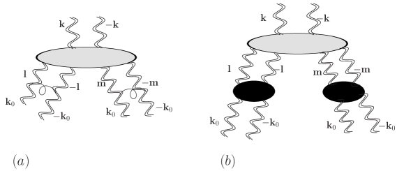
Figure 6: (a) The TPV with two BFKL interactions attached to it. (b) The TPV with gluon ladders.

Let us compute the collinear approximation to the BFKL kernels which, when convoluted with the TPV, will give a logarithmic integral. The expression for the emission part of the BFKL kernel is:

$$K(\textbf{q}_{1},\textbf{q}_{2};\textbf{k}_{1},\textbf{k}_{2})=-N_{c}g^{2}\bigg{[}(\textbf{k}_{1}+\textbf{k}_{2})^{2}-\frac{\textbf{q}_{2}^{2}\textbf{k}_{1}^{2}}{(\textbf{k}_{2}-\textbf{q}_{2})^{2}}-\frac{\textbf{q}_{1}^{2}\textbf{k}_{2}^{2}}{(\textbf{k}_{1}-\textbf{q}_{1})^{2}}\bigg{]}.$$ (27)

The factor $-N_{c}$ replaces the color tensors in eq.(8), since we have projected on the color singlet state. Assuming zero momentum transfer and $\textbf{q}^{2}_{1}\!>\!\!\!>\!\textbf{k}^{2}_{2}$ we get:

$$K\!=g^{2}N_{c}2\textbf{k}_{1}^{2},$$ (28)

where, in order to simplify the notation, we have skipped the arguments of the kernel $K$. Using this approximation in the formula for Fig.6a, we get the following expression for the convolution of the vertex with two BFKL kernels (one kernel for each two-gluon pair below the vertex):

$$(K\,K)\otimes{{\cal V}_{LON_{c}}^{r\{a^{\prime}\}\{b\}}}^{\tau=4} \,=\, \delta^{a_{1}^{\prime},a_{2}^{\prime}}\delta^{b_{1},b_{2}}\delta^{b_{3},b_{4}}\frac{\sqrt{2}\pi}{N_{c}^{2}-1}N_{c}^{2}2\textbf{k}^{2}\frac{g^{8}}{2}\cdot$$ (29)

$$\int_{\textbf{k}_{0}^{2}}^{\textbf{k}^{2}}\frac{d^{2}\textbf{l}}{(2\pi)^{3}}\int_{\textbf{k}_{0}^{2}}^{\textbf{k}^{2}}\frac{d^{2}\textbf{m}}{(2\pi)^{3}}\frac{2\textbf{k}_{0}^{2}}{\textbf{l}^{4}}\frac{2\textbf{k}_{0}^{2}}{\textbf{m}^{4}}\frac{4(2(\textbf{l}\!\cdot\!\textbf{m})^{2}-\textbf{l}^{2}\textbf{m}^{2})}{\textbf{k}^{4}}$$

$$= 0,$$

where $\textbf{k}_{0}$ is the lowest momentum scale which we do not specify at present. We notice that the integrals of l and m are logarithmic, but - what is most striking - the angular integral over the angle between l and m renders the Triple Pomeron Vertex to vanish. It is straightforward to iterate the convolution with BFKL kernels (Fig. 6b), and, as a result, we arrive at the conclusion that - after averaging over the azimuthal angles - the twist-four part of the TPV vertex gives zero contribution.

3.2 The virtual part

So far we have investigated contributions coming from the real part of the vertex. What remains are the disconnected parts. In order to investigate logarithmic contributions of the virtual pieces we have to convolute them with an impact factor at the upper end of Fig.1b. To deal with infrared finite quantities it is convenient to work with the impact factor of the photon. The function $G_{2}(\textbf{k}_{1},\textbf{k}_{2}+\textbf{k}_{4},\textbf{k}_{3})=G_{2}(\textbf{k}_{1},\textbf{k}_{3})$ (5) in the forward direction reads:

$$G_{2}(\textbf{k}_{1},\textbf{k}_{3})=-\textbf{k}^{4}\frac{1}{8\pi^{2}}\left(\ln\frac{|\textbf{k}_{1}|^{2}}{|\textbf{k}_{1}+\textbf{k}_{3}|^{2}}\delta^{(2)}(\textbf{k}_{1}-\textbf{k})+\ln\frac{|\textbf{k}_{3}|^{2}}{|\textbf{k}_{1}+\textbf{k}_{3}|^{2}}\delta^{(2)}(\textbf{k}_{3}+\textbf{k})\right).$$ (30)

The photon impact factor (for transversely polarized photons) has the form  [20, 21]

$$\phi_{a_{1}^{\prime}a_{2}^{\prime}}(\textbf{k},Q)=\delta^{a_{1}^{\prime}a_{2}^{\prime}}\alpha_{s}\alpha_{em}\sum_{q}e_{q}^{2}\int_{0}^{1}d\tau d\rho\frac{[\rho^{2}-(1-\rho)^{2}][\tau^{2}-(1-\tau)^{2}]\textbf{k}^{2}}{\rho(1-\rho)Q^{2}+\tau(1-\tau)\textbf{k}^{2}},$$ (31)

where $Q^{2}$ and $\textbf{k}^{2}$ denote the (negative) photon and gluon virtualities, resp. In this expression $\rho$ denotes the longitudinal component of the quark loop momentum (in the Sudakov decomposition), while the second integration variable $\tau$ is a Feynman parameter. For our investigations we are interested in the twist expansion. To perform the twist expansion of the impact factor one has to perform the Mellin transform with respect to $\textbf{k}^{2}/Q^{2}$. With the Mellin transform (15) one finds:

$$\phi_{a_{1}^{\prime}a_{2}^{\prime}}(\textbf{k},Q)=\int\frac{d\gamma}{2\pi i}\left(\frac{\textbf{k}^{2}}{Q^{2}}\right)^{-\gamma}\phi_{a_{1}^{\prime}a_{2}^{\prime}}(\gamma),$$ (32)

and we obtain:

$$\phi_{a_{1}^{\prime}a_{2}^{\prime}}(\gamma)=\delta^{a_{1}^{\prime}a_{2}^{\prime}}{\cal C}\frac{\Gamma(3+\gamma)}{\frac{5}{2}+\gamma}\frac{\Gamma(1+\gamma)}{1+\gamma}\frac{\Gamma(-\gamma)}{-\gamma}\frac{\Gamma(-\gamma+2)}{\Gamma(-\gamma+\frac{3}{2})}.$$ (33)

Turning to Fig.2b, we are interested in the following ordering of momenta: $|Q_{1}|\!\gg\!|\mbox{\boldmath{$\kappa$}}|\!\gg\!|\mbox{\boldmath{$\kappa$}}^{\prime}|\!\gg\!|Q_{0}|$. To analyse the twist-4 term of this kinematic region we need, for the upper impact factor, the twist-4 term. Closing, in eq.(32), the contour of the $\gamma$ integration to the left we obtain the following collinear expansion of the photon impact factor:

$$\phi_{a_{1}^{\prime}a_{2}^{\prime}}(\mbox{\boldmath{$\kappa$}},Q_{1})=\delta^{a_{1}^{\prime}a_{2}^{\prime}}\phi(\mbox{\boldmath{$\kappa$}},Q_{1})\,=\,\delta^{a_{1}^{\prime}a_{2}^{\prime}}{\cal C}\Bigg{\{}\left[\frac{14}{9}-\frac{4}{3}\ln\left(\frac{\mbox{\boldmath{$\kappa$}}^{2}}{Q_{1}^{2}}\right)\right]\frac{\mbox{\boldmath{$\kappa$}}^{2}}{Q_{1}^{2}}+\frac{2}{5}\left(\frac{\mbox{\boldmath{$\kappa$}}^{2}}{Q_{1}^{2}}\right)^{2}+...\Bigg{\}}\,,$$ (34)

where ${\cal C}=\sum_{f}e_{f}^{2}\alpha_{s}\alpha_{em}$. As it is well-known, the twist-four term has no logarithmic enhancement.

For later purposes we also list the results for the lower impact factor: we close the contour to the right and find:

$$\phi_{a_{1}^{\prime}a_{2}^{\prime}}(\mbox{\boldmath{$\kappa$}}^{\prime},Q_{0})=\delta^{a_{1}^{\prime}a_{2}^{\prime}}\phi(\mbox{\boldmath{$\kappa$}}^{\prime},Q_{0})\,=\,\delta^{a_{1}^{\prime}a_{2}^{\prime}}{\cal C}\Bigg{\{}\left[\frac{14}{9}-\frac{4}{3}\ln\left(\frac{Q_{0}^{2}}{{\mbox{\boldmath{$\kappa$}}^{\prime}}^{2}}\right)\right]+\frac{2}{5}\left(\frac{Q_{0}^{2}}{{\mbox{\boldmath{$\kappa$}}^{\prime}}^{2}}\right)^{.}..\Bigg{\}}.$$ (35)

For our twist-4 analysis of Fig.2b we will need the second term on the rhs.

Returning to the upper impact factor and concentrating on the twist-4 piece, we now easily see, by simply counting powers of momenta, that the virtual contributions of the TPV cannot contribute to the maximal power of logarithms. Namely, beginning with the impact factor above the TVP, we have the power $\textbf{k}^{4}$ which cancels the two gluon propagators attached to the impact factor. From the $G_{2}$ functions we find another power, $\textbf{k}^{4}$, which, through the $\delta$-functions, turns into $\textbf{m}^{4}$, $\textbf{l}^{4}$, or $(\textbf{m}\pm\textbf{l})^{4}$. When dividing the region of integration into the two parts $\textbf{m}\ll\textbf{l}$ and $\textbf{l}\ll\textbf{m}$, the terms with $(\textbf{m}\pm\textbf{l})^{4}$ turn into $\textbf{l}^{4}$ or $\textbf{m}^{4}$. Below the TPV we have the pairs of propagators, $1/\textbf{m}^{4}$, and $1/\textbf{l}^{4}$, and there is no m (or l)- dependent contribution from the BFKL kernels. Combining these momentum factors, we therefore obtain only integrals of the form

$$\int\frac{d^{2}l}{\textbf{l}^{4}}\int\frac{d^{2}m}{\textbf{m}^{4}}\textbf{l}^{4}$$

or

$$\int\frac{d^{2}l}{\textbf{l}^{4}}\int\frac{d^{2}m}{\textbf{m}^{4}}\textbf{m}^{4},$$

i.e.none of the integrals is logarithmic (this argument remains unaffected if we include the logarithms from the $G_{2}$ functions). Hence, within the leading-log approximation, also the virtual part of the TPV is zero.

Let us emphasize that our search for the ’maximal power of transverse logs’ is exactly what is required for a consistent twist-four analysis. In order to obtain this maximal power (i.e. one power for each transverse momentum loop integral), we had to start, at the upper impact factor with the twist-four term. Including a BFKL-ladder between the impact factor and the TPV forces us to take also the twist-four approximation of the kernel, i.e. instead of the leading twist approximation in (27), terms of the order ${\cal O}(\textbf{k}_{1}^{2}\frac{\textbf{k}_{1}^{2}}{\textbf{q}_{1}^{2}})$. Next, at the TPV we searched for terms of the order $\frac{\textbf{m}^{2}\textbf{l}^{2}}{\textbf{k}^{2}}$, and, finally, for the two BFKL kernels below the TPV, again the twist-2 approximation (27). It is only this sequence of approximations which provides one logarithm for each loop, i.e. otherwise we loose one (or more) powers of logarithmic enhancements. Our result then says that one coefficient in this sequence of terms, namely the TPV, vanishes and thus makes the twist-four term in the twist expansion (in the leading-log approximation) disappear.

3.3 Generalization to all higher twists

The main result of the previous subsections - the absence of collinear logarithms in the case of angular averaged BFKL ladders - can be generalized to all orders of powers of $1/Q^{2}$. We return to the function $V$ in (2) which is expressed in terms of the functions $G_{1}$ and $G_{2}$, and we average over the angles of m and l. First $G_{1}$:

$$G_{1}(\textbf{l},\textbf{m})=\frac{\textbf{k}^{2}\textbf{l}^{2}}{(\textbf{k}-\textbf{l})^{2}}+\frac{\textbf{k}^{2}\textbf{m}^{2}}{(\textbf{k}+\textbf{m})^{2}}-\frac{\textbf{k}^{4}(\textbf{l}+\textbf{m})^{2}}{(\textbf{k}-\textbf{l})^{2}(\textbf{k}+\textbf{m})^{2}}.$$ (36)

Let us denote the first term in this formula by A, the second one by B and the third one by C, the angle between l and m by $\alpha$, and the angle between m and k by $\beta$ (the angle between l and k then equals $2\pi-\alpha\!-\!\beta$). For the integrals over $\alpha$ and $\beta$ we find:

$$I_{A}=\frac{1}{(2\pi)^{2}}\int_{0}^{2\pi}\!\!d{\alpha}\int_{0}^{2\pi}\!\!d{\beta}\,A=\frac{\textbf{k}^{2}\textbf{l}^{2}}{|\textbf{l}^{2}-\textbf{k}^{2}|}$$ (37)

and:

$$I_{B}=\frac{1}{(2\pi)^{2}}\int_{0}^{2\pi}d{\alpha}\int_{0}^{2\pi}d{\beta}\,B=\frac{\textbf{k}^{2}\textbf{m}^{2}}{|\textbf{m}^{2}-\textbf{k}^{2}|}.$$ (38)

To compute the integral over $C$ we split $C=C_{1}+C_{2}+C_{3}$ into three pieces. The corresponding integrals are:

$$I_{C_{1}}=\frac{1}{(2\pi)^{2}}\int_{0}^{2\pi}\!\!d\alpha d\beta\frac{\textbf{k}^{4}\textbf{l}^{2}}{(\textbf{k}^{2}-2\textbf{l}\textbf{k}\cos(\alpha+\beta)+\textbf{l}^{2})(\textbf{k}^{2}+2\textbf{m}\textbf{k}\cos\beta+\textbf{m}^{2})},$$ (39)

$$I_{C_{2}}=\frac{1}{(2\pi)^{2}}\int_{0}^{2\pi}\!\!d\alpha d\beta\frac{2\textbf{k}^{4}|\textbf{l}||\textbf{m}|\cos\alpha}{(\textbf{k}^{2}-2\textbf{l}\textbf{k}\cos(\alpha+\beta)+\textbf{l}^{2})(\textbf{k}^{2}+2\textbf{m}\textbf{k}\cos\beta+\textbf{m}^{2})},$$ (40)

$$I_{C_{3}}=\frac{1}{(2\pi)^{2}}\int_{0}^{2\pi}d\alpha d\beta\frac{\textbf{k}^{4}\textbf{m}^{2}}{(\textbf{k}^{2}-2\textbf{l}\textbf{k}\cos(\alpha+\beta)+\textbf{l}^{2})(\textbf{k}^{2}+2\textbf{m}\textbf{k}\cos\beta+\textbf{m}^{2})}.$$ (41)

The results of the integration are:

$$I_{C_{1}}=\frac{\textbf{l}^{2}\textbf{k}^{4}}{|\textbf{l}^{2}-\textbf{k}^{2}||\textbf{m}^{2}-\textbf{k}^{2}|},$$ (42)

$$I_{C_{2}}=\frac{-8\textbf{l}^{2}\textbf{m}^{2}\textbf{k}^{6}}{|\textbf{l}^{2}-\textbf{k}^{2}||\textbf{m}^{2}-\textbf{k}^{2}|(\textbf{l}^{2}+\textbf{k}^{2}+|\textbf{l}^{2}-\textbf{k}^{2}|)(\textbf{m}^{2}+\textbf{k}^{2}+|\textbf{m}^{2}-\textbf{k}^{2}|)},$$ (43)

$$I_{C_{3}}=\frac{\textbf{m}^{2}\textbf{k}^{4}}{|\textbf{l}^{2}-\textbf{k}^{2}||\textbf{m}^{2}-\textbf{k}^{2}|}.$$ (44)

The total contribution is given by summing up $I_{A}$, $I_{B}$, $I_{C_{1}}$, $I_{C_{2}}$ , $I_{C_{3}}$ The result can greatly be simplified if we consider special situations. For instance, if $\textbf{k}^{2}\!\ll\textbf{l}^{2},\textbf{m}^{2}$, we may drop the absolute value signs. Adding all terms we obtain:

$$\sum_{A,..,C_{3}}I=\frac{2\textbf{l}^{2}\textbf{m}^{2}\textbf{k}^{2}-2\textbf{l}^{2}\textbf{k}^{4}-2\textbf{b}^{2}\textbf{k}^{4}+2\textbf{k}^{6}}{(\textbf{l}^{2}-\textbf{k}^{2})(\textbf{m}^{2}-\textbf{k}^{2})}=2\textbf{k}^{2}.$$ (45)

In all other cases: $\textbf{k}^{2}\!\gg\textbf{l}^{2},\textbf{m}^{2}$, $\textbf{m}^{2}\!\!\gg\!\!\textbf{k}^{2}\!\!\gg\!\!\textbf{l}^{2}$, or $\textbf{l}^{2}\!\!\gg\textbf{k}^{2}\!\!\gg\!\!\textbf{m}^{2}$ the sum of all terms gives zero. Therefore the final result can be simply written as:

$$\frac{1}{(2\pi)^{2}}\int_{0}^{2\pi}\!\!d\alpha d\beta G_{1}(\textbf{l},\textbf{m})=2\textbf{k}^{2}\theta(\textbf{l}^{2}-\textbf{k}^{2})\theta(\textbf{m}^{2}-\textbf{k}^{2}),$$ (46)

where the factor $1/(2\pi)^{2}$ comes from averaging.

Let us now perform the angular averaging of the disconnected pieces of the $G(\textbf{l},\textbf{m})$ function. We have:

$$G_{2}(\textbf{l},\textbf{m})=-\textbf{k}^{4}\frac{1}{8\pi^{2}}\left(\ln\frac{\textbf{l}^{2}}{(\textbf{l}+\textbf{m})^{2}}\delta^{(2)}(\textbf{l}-\textbf{k})+\ln\frac{\textbf{m}^{2}}{(\textbf{l}+\textbf{m})^{2}}\delta^{(2)}(\textbf{m}-\textbf{k})\right).$$ (47)

To compute the integral over angles we split the region of integration. In the case when $|\textbf{m}|\!\!\gg\!\!|\textbf{l}|$ the first term gives

$$I_{D}=\frac{1}{(2\pi)^{2}}\int_{0}^{2\pi}d\alpha d\beta\ln\frac{\textbf{l}^{2}}{\textbf{l}^{2}+\textbf{m}^{2}+2\textbf{l}\textbf{m}\cos\alpha}=\ln\frac{\textbf{l}^{2}}{\textbf{m}^{2}},$$ (48)

whereas the second one vanishes. In the case when $|\textbf{l}|\!\!\gg\!\!|\textbf{m}|$ we obtain zero from the first term and

$$I_{D}=\frac{1}{(2\pi)^{2}}\int_{0}^{2\pi}d\alpha d\beta\ln\frac{\textbf{m}^{2}}{\textbf{l}^{2}+\textbf{m}^{2}+2\textbf{l}\textbf{m}\cos\alpha}=\ln\frac{\textbf{m}^{2}}{\textbf{l}^{2}}$$ (49)

from the second one. We combine the two cases in the following way:

$$G_{2}(\textbf{l},\textbf{m})=-\textbf{k}^{4}\frac{1}{8\pi^{2}}\left(\ln\frac{\textbf{l}^{2}}{\textbf{m}^{2}}\theta(\textbf{m}^{2}-\textbf{l}^{2})\delta^{(2)}(\textbf{l}-\textbf{k})+\ln\frac{\textbf{m}^{2}}{\textbf{l}^{2}}\theta(\textbf{l}^{2}-\textbf{m}^{2})\delta^{(2)}(\textbf{m}-\textbf{k})\right).$$ (50)

Putting all pieces together and including the remaining $G$ functions we arrive at the angular-averaged form of $V$:

$$\frac{1}{(2\pi)^{2}}\int_{0}^{2\pi}d\alpha d\beta V(\textbf{k},-\textbf{k};\textbf{l},-\textbf{l},\textbf{m},-\textbf{m})=4\frac{g^{4}}{2}\bigg{[}2\textbf{k}^{2}\theta(\textbf{l}^{2}-\textbf{k}^{2})\theta(\textbf{m}^{2}-\textbf{k}^{2})$$

$$+\frac{1}{8\pi^{2}}\bigg{(}\ln\left(\frac{\textbf{l}^{2}}{\textbf{m}^{2}}\right)\delta^{(2)}(\textbf{l}-\textbf{k})\theta(\textbf{m}^{2}-\textbf{l}^{2})+\ln\left(\frac{\textbf{m}^{2}}{\textbf{l}^{2}}\right)\delta^{(2)}(\textbf{m}-\textbf{k})\theta(\textbf{l}^{2}-\textbf{m}^{2})\bigg{)}\bigg{]}.$$ (51)

The presence of the $\theta$-functions forbids all collinear configurations, i.e. there is no expansion in inverse powers of $\textbf{k}^{2}$. The physical meaning of this result is the following: if the two pomerons entering the vertex from below have smaller momenta than the pomeron from above, they cannot resolve it and cannot merge because they do not feel ’color’ and the vertex vanishes. In the language of a twist-expansion, our result states that, in the leading-log approximation, not only twist-four, but all higher twist terms are zero, provided we restrict ourselves to the large-$N_{c}$ limit, and we use only the BFKL ladders with conformal spin zero below the TPV.

4 The anticollinear limit

4.1 Real part

Let us now investigate the anticollinear limit of the $2\to 4$ vertex (Fig.7). In contrast to the collinear limit where the BFKL ladders below the vertex had to be in the forward direction, the anticollinear configuration allows for a nonzero momentum transfer across the BFKL ladders above the vertex. The momentum transfer here, as we will see, does not lead to a loss of a logarithm. We are interested in the limit $|\textbf{w}|\!\!<\!<\!\!|\textbf{w}_{1}|\!,|\textbf{w}_{2}|\!,|\textbf{w}_{3}|\!,|\textbf{w}_{4}|$. To study the real emission part of the TPV it is convenient to rewrite the $G_{1}$ function in the form:

$$G_{1}(\textbf{w}_{1},\textbf{w}_{2}+\textbf{w}_{3},\textbf{w}_{4})=\textbf{w}^{2}\left[\frac{1}{(1-2\frac{\textbf{w}\cdot\textbf{w}_{1}}{\textbf{w}_{1}^{2}}+\frac{\textbf{w}^{2}}{\textbf{w}_{1}^{2}})}+\frac{1}{(1+2\frac{\textbf{w}\cdot\textbf{w}_{4}}{\textbf{w}_{4}^{2}}+\frac{\textbf{w}^{2}}{\textbf{w}_{4}^{2}})}\right.$$

$$\left.-\textbf{w}^{2}\frac{(\textbf{w}_{1}+\textbf{w}_{4})^{2}}{\textbf{w}_{1}^{2}\textbf{w}_{4}^{2}}\frac{1}{(1-2\frac{\textbf{w}\cdot\textbf{w}_{1}}{\textbf{w}_{1}^{2}}+\frac{\textbf{w}^{2}}{\textbf{w}_{1}^{2}})(1+2\frac{\textbf{w}\cdot\textbf{w}_{4}}{\textbf{w}_{4}^{2}}+\frac{\textbf{w}^{2}}{\textbf{w}_{4}^{2}})}\right].$$ (52)

Here we have used the momentum conservation $\sum_{i}\textbf{w}_{i}=0$. The expansion parameters are $|\textbf{w}|/|\textbf{w}_{1}|$ and $|\textbf{w}|/|\textbf{w}_{3}|$. Performing the expansion we obtain up to second order:

$$G_{1}(\textbf{w}_{1},\textbf{w}_{2}+\textbf{w}_{3},\textbf{w}_{4})=\textbf{w}^{2}\left[2+2\frac{\textbf{w}\!\cdot\!\textbf{w}_{1}}{\textbf{w}_{1}^{2}}-2\frac{\textbf{w}\!\cdot\!\textbf{w}_{4}}{\textbf{w}_{4}^{2}}\right.$$

$$\left.-2\frac{\textbf{w}^{2}}{\textbf{w}_{1}^{2}}-2\frac{\textbf{w}^{2}}{\textbf{w}_{4}^{2}}-2\textbf{w}^{2}\frac{\textbf{w}_{1}\!\cdot\!\textbf{w}_{4}}{\textbf{w}_{1}^{2}\textbf{w}_{4}^{2}}+\left(2\frac{\textbf{w}\!\cdot\!\textbf{w}_{1}}{\textbf{w}_{1}^{2}}\right)^{2}+\left(2\frac{\textbf{w}\!\cdot\!\textbf{w}_{4}}{\textbf{w}_{4}^{2}}\right)^{2}+...\right].$$ (53)

Using (4) we obtain for the leading term of the TPV:

$${\cal V}_{LON_{c}}^{r\{a^{\prime}\}}(\textbf{p},-\textbf{p}-\textbf{r},\textbf{q},-\textbf{q}+\textbf{r})^{leading}=\delta^{a_{1}^{\prime},a_{2}^{\prime}}\delta^{b_{1},b_{2}}\delta^{b_{3},b_{4}}\frac{\sqrt{2}\pi}{N_{c}^{2}-1}\frac{g^{4}}{2}2\textbf{w}^{2}.$$ (54)

One easily sees that this term does not provide logarithms in the momentum scale. The subsequent terms in (53) vanish after averaging over the angle of w. Therefore, in order to get, after convolution with BFKL kernels in the subsystems $(12)$ and $(34)$, the required logarithmic contribution we need to consider, in (53), terms of higher order. After averaging over the angle of w, and after summing, in (4), over all the $G_{1}$ functions, the resulting contribution is the following:

$${\cal V}_{LON_{c}}^{r\{a^{\prime}\}}(\textbf{w}_{1},\textbf{w}_{2},\textbf{w}_{3},\textbf{w}_{4})^{\tau=-2}=$$

$$\begin{split}\delta^{a_{1}^{\prime},a_{2}^{\prime}}\delta^{b_{1},b_{2}}\delta^{b_{3},b_{4}}\frac{\sqrt{2}\pi}{N_{c}^{2}-1}g^{4}\textbf{w}^{4}\Bigg{[}-\frac{\textbf{w}_{1}\!\cdot\!\textbf{w}_{3}}{\textbf{w}_{1}^{2}\textbf{w}_{3}^{2}}-\frac{\textbf{w}_{2}\!\cdot\!\textbf{w}_{3}}{\textbf{w}_{2}^{2}\textbf{w}_{3}^{2}}-\frac{\textbf{w}_{1}\!\cdot\!\textbf{w}_{4}}{\textbf{w}_{1}^{2}\textbf{w}_{4}^{2}}-\frac{\textbf{w}_{2}\!\cdot\!\textbf{w}_{4}}{\textbf{w}_{2}^{2}\textbf{w}_{4}^{2}}\\ -\frac{\textbf{w}_{1}\!\cdot\!(\textbf{w}_{1}+\textbf{w}_{2})}{\textbf{w}_{1}^{2}(\textbf{w}_{1}+\textbf{w}_{2})^{2}}-\frac{\textbf{w}_{2}\!\cdot\!(\textbf{w}_{1}+\textbf{w}_{2})}{\textbf{w}_{2}^{2}(\textbf{w}_{1}+\textbf{w}_{2})^{2}}-\frac{\textbf{w}_{3}\!\cdot\!(\textbf{w}_{3}+\textbf{w}_{4})}{\textbf{w}_{3}^{2}(\textbf{w}_{3}+\textbf{w}_{4})^{2}}-\frac{\textbf{w}_{4}\!\cdot\!(\textbf{w}_{3}+\textbf{w}_{4})}{\textbf{w}_{4}^{2}(\textbf{w}_{3}+\textbf{w}_{4})^{2}}\\ -\frac{(\textbf{w}_{1}+\textbf{w}_{2})\!\cdot\!(\textbf{w}_{3}+\textbf{w}_{4})}{(\textbf{w}_{1}+\textbf{w}_{2})^{2}(\textbf{w}_{3}+\textbf{w}_{4})^{2}}\Bigg{]}.\end{split}$$ (55)

To proceed further we need the anticollinear limit of the BFKL kernel. Using (27), setting $\textbf{k}_{1}=\textbf{w}_{1}$, $\textbf{k}_{2}=\textbf{w}_{2}$ and requiring that $|\textbf{q}_{1}|\!\!\gg\!\!|\textbf{w}_{1}|\!,|\textbf{w}_{2}|$ we obtain:

$$K=-\,g^{2}N_{c}2\textbf{w}_{1}\!\cdot\!\textbf{w}_{2}.$$ (56)

As already mentioned before we are interested in the maximal power of logarithms in the momentum scale; this leads to the particular momentum configuration, where the momentum transfer across the BFKL Pomerons in the subsystems $(12)$ and $(34)$ is nonzero. (note that below the vertex we are still in the forward direction). We set: $\textbf{w}_{1}\!\!=\!\textbf{p}$, $\textbf{w}_{2}\!\!=\!-\textbf{p}\!-\!\textbf{r}$,$\textbf{w}_{3}\!=\!\textbf{q}$, $\textbf{w}_{4}\!=\!-\textbf{q}\!+\!\textbf{r}$.

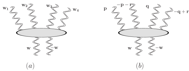
Figure 7: Momentum assignments at the lower TPV.

In order to obtain, after convoluting with BFKL kernels in the subsystems $(12)$ and $(34)$, logarithmic contributions, we have to consider the following momentum-ordered configurations:

• The configuration where $|\textbf{r}|\!\!\gg\!|\textbf{p}|\!\gg\!|\textbf{q}|$. BFKL kernels and propagators are of the form:

  $$N_{c}g^{2}2\textbf{p}\!\cdot\!\textbf{r},\,\,\,\,\,-N_{c}g^{2}2\textbf{q}\!\cdot\!\textbf{r}$$ (57)

  and

  $$\frac{1}{\textbf{p}^{2}\textbf{r}^{2}}\,\,,\,\,\frac{1}{\textbf{q}^{2}\textbf{r}^{2}},$$ (58)

  resp. In order to render all transverse momemtum integrations (in p, q, and in r) logarithmic, we need, from the TVP, terms proportional to $\frac{\textbf{p}\!\cdot\!\textbf{q}}{\textbf{p}^{2}\textbf{q}^{2}}$: they are obtained from the first term in (55):

  $${\cal V}_{LON_{c}}^{r\{a^{\prime}\},\{b\},\tau=-2}(\textbf{p},-\textbf{p}-\textbf{r},\textbf{q},-\textbf{q}+\textbf{r})=-\delta^{a_{1}^{\prime},a_{2}^{\prime}}\delta^{b_{1},b_{2}}\delta^{b_{3},b_{4}}\frac{\sqrt{2}\pi}{N_{c}^{2}-1}g^{4}\textbf{w}^{4}\frac{\textbf{p}\!\cdot\!\textbf{q}}{\textbf{p}^{2}\textbf{q}^{2}}.$$ (59)

  Combining these expressions and performing the integrals we obtain:

  $$(K_{1}\,K_{2})\otimes{\cal V}_{LON_{c}}^{r\{a^{\prime}\},\{b\},\tau=-2}=\delta^{a_{1}^{\prime},a_{2}^{\prime}}\delta^{b_{1},b_{2}}\delta^{b_{3},b_{4}}\frac{\sqrt{2}\pi}{N_{c}^{2}-1}N_{c}^{2}\!\!\frac{g^{8}}{8(2\pi)^{3}}\!\frac{\textbf{w}^{4}}{3!}\!\!\!\left(\ln\frac{\textbf{w}_{0}^{2}}{\textbf{w}^{2}}\right)^{3},$$ (60)

  where $|\!\textbf{w}_{0}\!|$ is the momentum at the upper end of the BFKL kernels, specified by the condition that it should be smaller than the momentum scales $|\textbf{l}|$ and $|\textbf{m}|$ which were considered in the collinear limit of the upper TPV. Convoluting this expression with the impact factor $\phi_{\{b^{\prime}\}}(\textbf{w})=\delta^{b_{1}^{\prime}b_{2}^{\prime}}\frac{2}{5}{\cal C}\frac{Q_{0}^{2}}{\textbf{w}^{2}}\ln Q_{0}^{2}/\textbf{w}^{2}$ below the vertex yields:

  $$\begin{split}(K_{1}\,K_{2})\otimes{\cal V}_{LON_{c}}^{r\{a^{\prime}\},\{b\},\tau=-2}\otimes\phi_{\{a^{\prime}\}}=\delta^{b_{1},b_{2}}\delta^{b_{3},b_{4}}\sqrt{2}\pi N_{c}^{2}\frac{2}{5}{\cal C}\frac{\alpha_{s}^{4}}{2\pi}\frac{Q_{0}^{2}}{4!}\left(\ln\frac{\textbf{w}_{0}^{2}}{Q_{0}^{2}}\right)^{4}.\end{split}$$ (61)

  Here, in order to get the logarithmic contribution, we took, in (35), the next-to-leading term in the anticollinear expansion of $\phi$ . In the configuration $|\textbf{r}|\gg|\textbf{q}|\!\!\gg\!\!|\textbf{p}|$ the same result is obtained.

• Repeating a similar analysis in the case when $|\textbf{q}|\!\!\gg\!|\textbf{p}|\!\!\gg\!\!|\textbf{r}|$, we find, from the last term on the rhs of (55):

  $$(K_{1}\,K_{2})\otimes{\cal V}_{LON_{c}}^{r\{a^{\prime}\},\{b\},\tau=-2}\otimes\phi_{\{a^{\prime}\}}=\delta^{b_{1},b_{2}}\delta^{b_{3},b_{4}}\sqrt{2}\pi N_{c}^{2}\frac{2}{5}{\cal C}\frac{2\alpha_{s}^{4}}{\pi}\frac{Q_{0}^{2}}{4!}\left(\ln\frac{\textbf{w}_{0}^{2}}{Q_{0}^{2}}\right)^{4}.$$ (62)

  The same contribution is obtained from the region $|\textbf{p}|\!\!\gg\!|\textbf{q}|\!\!\gg\!\!|\textbf{r}|$.

• Finally, there are the regions $|\textbf{q}|\!\gg\!\!|\textbf{r}|\gg\!\!|\textbf{p}|$ and $|\textbf{p}|\!\gg\!\!|\textbf{r}|\!\gg\!|\textbf{q}|$. For the first case we use the first term in the second line of (55) and obtain:

  $$(K_{1}\,K_{2})\otimes{\cal V}_{LON_{c}}^{r\{a^{\prime}\},\{b\},\tau=-2}\otimes\phi_{\{a^{\prime}\}}=\delta^{b_{1},b_{2}}\delta^{b_{3},b_{4}}\sqrt{2}\pi N_{c}^{2}\frac{2}{5}{\cal C}\frac{\alpha_{s}^{4}}{\pi}\frac{Q_{0}^{2}}{4!}\left(\ln\frac{\textbf{w}_{0}^{2}}{Q_{0}^{2}}\right)^{4}.$$ (63)

  The second region gives the same contribution.

4.2 Virtual parts

Let us now analyze the contribution coming from the virtual parts of the vertex in the anticollinear limit. Again, we are looking for the maximal power of logarithms. We begin with the region $|\textbf{r}|\gg|\textbf{p}|,|\textbf{q}|$. Using (2),(30) for the virtual parts of the TPV, (57) for the BFKL kernel, (58) for the propagators above the vertex, and (35) for the lower impact factor we immediately see that none of the $G_{2}$ functions allows for three logarithmic integrals. The same observation holds for the regions $|\textbf{q}|\!\gg\!\!\!|\textbf{r}|\gg\!\!|\textbf{p}|$ and $|\textbf{p}|\!\gg\!\!|\textbf{r}|\gg\!|\textbf{q}|$. We are then left with the region $|\textbf{p}|,|\textbf{q}|\gg|\textbf{r}|$. From the BFKL kernels and from the propagators we find the denominators $1/\textbf{p}^{2}\cdot 1/\textbf{q}^{2}$, and we therefore need the factor $1/\textbf{r}^{2}$ from the propagators below the TPV. They can come only from the first term in the function $G_{2}(1+2,3,4)$:

$$g^{2}G_{2}(1+2,3,4)=\alpha_{s}\frac{\textbf{w}^{4}}{2\pi}\left(\ln\frac{\textbf{w}_{3}^{2}}{(\textbf{w}_{3}+\textbf{w}_{4})^{2}}\,\,\delta(\textbf{w}+\textbf{w}_{3}+\textbf{w}_{4})+\ln\frac{\textbf{w}_{3}^{2}}{\textbf{w}_{4}^{2}}\,\,\delta(\textbf{w}+\textbf{w}_{4})\right),$$ (64)

and from analogous terms in $G_{2}(1+2,3,4)$, $G_{2}(1,2,3+4)$, $G_{2}(2,1,3+4)$. Convoluting these $G_{2}$ functions with the BFKL kernels and with the impact factor, and setting the lowest momentum scale equal to $Q_{0}^{2}$, we find:

$$(K_{1}\,K_{2})\otimes{\cal V}_{LON_{c}}^{vl\{a^{\prime}\},\{b\}}\otimes\phi_{\{a^{\prime}\}}=-\delta^{b_{1},b_{2}}\delta^{b_{3},b_{4}}\sqrt{2}\pi N_{c}^{2}\frac{2}{5}{\cal C}\frac{\alpha_{s}^{4}}{\pi}\frac{Q_{0}^{2}}{2}\left(\ln\frac{\textbf{w}_{0}^{2}}{Q_{0}^{2}}\right)^{4}.$$ (65)

Let us shortly summarize our results for the large-$N_{c}$ limit, before we continue the finite $N_{c}$ analysis. Our goal was to find those terms of the twist expansion of the TPV which, after convolution with the BFKL kernel, would generate the maximal possible power of transverse momentum logarithms. In the collinear case (upper TPV), we had to restrict the BFKL ladders below the TPV to the forward direction, and we therefore expected to find, from the m and l integrations, two logarithms. After the convolution with the upper impact factor, a third logarithm should appear. What we found is that the coefficient of this maximal number of logarithms vanishes, both for the connected and for the disconnected parts of the TPV. In the anticollinear case we had to include the integral over the momentum transfer across the first BFKL kernel. After convoluting these integrals with the lower impact factor, we expect four logarithms. In fact, we found these logarithmic contributions, both in the real and in the virtual part of the TPV, and they came from different regions of ordered transverse momenta.

This completes our twist-4 analysis of the one-loop Pomeron self-energy of the BFKL Pomeron (Fig.2b). We have found that the upper TPV vanishes at the twist-4 point, whereas the lower one provides nonzero contributions.

5 Finite $N_{c}$

5.1 The collinear limit

In this section we are going to investigate contributions to the vertex in (17) that are suppressed in the large $N_{c}$ limit. Repeating our analysis of the previous sections we obtain for the first subleading piece:

$${\cal V}_{subN_{c}}^{r\{a^{\prime}\},\{b\}}(1,3,2,4)^{\tau=4}=$$

$$=\delta^{a_{1}^{\prime}a_{2}^{\prime}}\delta^{b_{1},b_{2}}\delta^{b_{3},b_{4}}\frac{\sqrt{2}\pi}{(N_{c}^{2}-1)^{2}}g^{4}\;\textbf{k}^{2}\frac{4(-\textbf{k}_{1}\!\cdot\!\textbf{k}_{3}\textbf{k}_{2}\!\cdot\!\textbf{k}_{4}+\textbf{k}_{1}\!\cdot\!\textbf{k}_{2}\textbf{k}_{3}\!\cdot\!\textbf{k}_{4}+\textbf{k}_{1}\!\cdot\!\textbf{k}_{4}\textbf{k}_{2}\!\cdot\!\textbf{k}_{3})}{\textbf{k}^{4}}.$$ (66)

Substituting $\textbf{k}_{1}=\textbf{l}$, $\textbf{k}_{2}=-\textbf{l}$, $\textbf{k}_{3}=\textbf{m}$, $\textbf{k}_{4}=-\textbf{m}$ we obtain:

$${\cal V}_{subN_{c}}^{r\{a^{\prime}\},\{b\}}(\textbf{l},\textbf{m},-\textbf{l},-\textbf{m})^{\tau=4}=\delta^{a_{1}^{\prime}a_{2}^{\prime}}\delta^{b_{1},b_{2}}\delta^{b_{3},b_{4}}\frac{\sqrt{2}\pi}{(N_{c}^{2}-1)^{2}}g^{4}\textbf{k}^{2}\frac{4\textbf{l}^{2}\textbf{m}^{2}}{\textbf{k}^{4}}.$$ (67)

The convolution with the two BFKL kernels gives:

$${\cal V}_{subN_{c}}^{r\{a^{\prime}\},\{b\},\tau=4}\otimes(K_{1}\,K_{2})=\delta^{a_{1}^{\prime}a_{2}^{\prime}}\delta^{b_{1},b_{2}}\delta^{b_{3},b_{4}}\frac{\sqrt{2}\pi}{(N_{c}^{2}-1)^{2}}N_{c}^{2}\frac{4g^{8}}{(2\pi)^{4}}\frac{\textbf{k}_{0}^{4}}{\textbf{k}^{2}}\left(\ln\frac{\textbf{k}^{2}}{\textbf{k}_{0}^{2}}\right)^{2}.$$ (68)

Convolution with the impact factor gives:

$$\phi_{\{a^{\prime}\}}\otimes{\cal V}_{subN_{c}}^{r\{a^{\prime}\},\{b\},\tau=4}\otimes(K_{1}\,K_{2})=\frac{\sqrt{2}\pi}{N_{c}^{2}-1}N_{c}^{2}\frac{2}{5}{\cal C}\frac{8\alpha_{s}^{4}}{\pi^{2}}\frac{\textbf{k}_{0}^{4}}{Q_{1}^{4}}\frac{1}{3}\left(\ln\frac{Q_{1}^{2}}{k_{0}^{2}}\right)^{3}.$$ (69)

The same result holds for the second subleading part.

For the virtual corrections to the TVP the situation is the same as for the leading-$N_{c}$ part: by simply inspecting the powers of transverse momenta, we find that the integrations over m and l are not logarithmic, i.e. they cannot generate the maximal power of logarithms.

5.2 The anticollinear limit

Here our starting expression for the real part of the TPV can be taken directly from the rhs of eq.(55), by interchanging $\textbf{w}_{2}$ and $\textbf{w}_{3}$. For the first nonleading piece we have:

$${\cal V}_{subN_{c}}^{r\{a^{\prime}\},\{b\}}(\textbf{w}_{1},\textbf{w}_{3},\textbf{w}_{2},\textbf{w}_{4})^{\tau=-2}=$$

$$\begin{split}\delta^{a_{1}^{\prime},a_{2}^{\prime}}\delta^{b_{1},b_{2}}\delta^{b_{3},b_{4}}\frac{\sqrt{2}\pi}{(N_{c}^{2}-1)^{2}}g^{4}\textbf{w}^{4}\Bigg{[}-\frac{\textbf{w}_{1}\!\cdot\!\textbf{w}_{2}}{\textbf{w}_{1}^{2}\textbf{w}_{2}^{2}}-\frac{\textbf{w}_{2}\!\cdot\!\textbf{w}_{3}}{\textbf{w}_{2}^{2}\textbf{w}_{3}^{2}}-\frac{\textbf{w}_{1}\!\cdot\!\textbf{w}_{4}}{\textbf{w}_{1}^{2}\textbf{w}_{4}^{2}}-\frac{\textbf{w}_{3}\!\cdot\!\textbf{w}_{4}}{\textbf{w}_{3}^{2}\textbf{w}_{4}^{2}}\\ -\frac{\textbf{w}_{1}\!\cdot\!(\textbf{w}_{1}+\textbf{w}_{3})}{\textbf{w}_{1}^{2}(\textbf{w}_{1}+\textbf{w}_{3})^{2}}-\frac{\textbf{w}_{3}\!\cdot\!(\textbf{w}_{1}+\textbf{w}_{3})}{\textbf{w}_{3}^{2}(\textbf{w}_{1}+\textbf{w}_{3})^{2}}-\frac{\textbf{w}_{2}\!\cdot\!(\textbf{w}_{2}+\textbf{w}_{4})}{\textbf{w}_{2}^{2}(\textbf{w}_{2}+\textbf{w}_{4})^{2}}-\frac{\textbf{w}_{4}\!\cdot\!(\textbf{w}_{2}+\textbf{w}_{4})}{\textbf{w}_{4}^{2}(\textbf{w}_{2}+\textbf{w}_{4})^{2}}\\ -\frac{(\textbf{w}_{1}+\textbf{w}_{3})\!\cdot\!(\textbf{w}_{2}+\textbf{w}_{4})}{(\textbf{w}_{1}+\textbf{w}_{3})^{2}(\textbf{w}_{2}+\textbf{w}_{4})^{2}}\Bigg{]}.\end{split}$$ (70)

The analysis is analogous to the leading-$N_{c}$ case. In detail we find:

• For $|\textbf{r}|\!\!\gg\!\!|\textbf{p}|\!\!\gg\!\!|\textbf{q}|$ the logarithmic contribution comes, on the rhs of eq.(70), from the second term of the second line. We obtain:

  $$(K_{1}\,K_{2})\otimes{\cal V}_{subN_{c}}^{r\{a^{\prime}\},\{b\}}\otimes\phi_{\{a^{\prime}\}}=\delta^{b_{1},b_{2}}\delta^{b_{3},b_{4}}\frac{\sqrt{2}\pi}{N_{c}^{2}-1}N_{c}^{2}\frac{2}{5}{\cal C}\frac{\alpha_{s}^{4}}{2\pi}\frac{Q_{0}^{2}}{4!}\left(\ln\frac{\textbf{w}_{0}^{2}}{Q_{0}^{2}}\right)^{4}.$$ (71)

  The same result holds for the region $|\textbf{r}|\!\gg\!|\textbf{q}|\!\gg\!|\textbf{p}|$, taking in eq.(70) the first term of the second line. This result is same as in (61), except for the suppression by $N_{c}^{2}-1$.

• $|\textbf{q}|\!\!\gg\!\!|\textbf{r}|\!\gg\!|\textbf{p}|$: here we use the first term on the rhs of eq.(70) and obtain

  $$(K_{1}\,K_{2})\otimes{\cal V}_{subN_{c}}^{r\{a^{\prime}\},\{b\}}\otimes\phi_{\{a^{\prime}\}}=\delta^{b_{1},b_{2}}\delta^{b_{3},b_{4}}\frac{\sqrt{2}\pi}{N_{c}^{2}-1}N_{c}^{2}\frac{2}{5}{\cal C}\frac{\alpha_{s}^{4}}{\pi}\frac{Q_{0}^{2}}{4!}\left(\ln\frac{\textbf{w}_{0}^{2}}{Q_{0}^{2}}\right)^{4}.$$ (72)

  The region $|\textbf{p}|\!\!¸\gg\!\!|\textbf{r}|\!\gg\!|\textbf{q}|$ gives the same result. It coincides with (63), but is suppressed by $N_{c}^{2}-1$.

The regions $|\textbf{q}|\!\!\!\gg\!\!\!|\textbf{p}|\!\!\!\gg\!\!\!|\textbf{r}|$ and $|\textbf{p}|\!\!\!\gg\!\!\!|\textbf{q}|\!\!\!\gg\!\!\!|\textbf{r}|$ do not contribute to the maximal number of logarithms.

Finally we come to the virtual parts of the $N_{c}$-suppressed parts of the TPV. Repeating the analysis, carried out for the virtual part of the leading-$N_{c}$ piece, we find no contribution to the maximal number of logarithms. The final result for the anticollinaer limit of the $N_{c}$-suppressed part of the TPV, therefore, is given by the real piece alone.

6 Nonlinear evolution equations

6.1 General evolution equations

Let us now make some use of the TPV in QCD reggeon field theory. To be definite let us consider deep inelastic scattering on a hadronic target (a single proton or a nucleus). We define color singlet $t$-channel states of $n$ reggeized gluons ($n$ even) in the Heisenberg picture which are labeled by color and momentum degrees of freedom:

$$|n\rangle = \frac{1}{\sqrt{n!}}a^{\dagger}_{a_{1}}(\textbf{k}_{1})...a^{\dagger}_{a_{n}}(\textbf{k}_{n})|0\rangle$$ (73)

$$= |\textbf{k}_{1},..\textbf{k}_{n};a_{1},..a_{n}\rangle.$$

The normalization is:

$$[a_{a}(\textbf{k}),a^{\dagger}_{a^{\prime}}(\textbf{k}^{\prime})]=(2\pi)^{3}\textbf{k}^{2}\delta(\textbf{k}-\textbf{k}^{\prime})\delta_{aa^{\prime}}$$ (74)

and

$$\langle n|n^{\prime}\rangle=\delta_{n^{\prime}n}\frac{1}{n^{\prime}!}\sum_{\sigma(n)}\prod_{i=1}^{n^{\prime}}\left((2\pi)^{3}\delta(\textbf{k}_{i}-\textbf{k}_{i}^{\prime})\textbf{k}_{i}^{2}\delta^{a_{i}a_{i}^{{}^{\prime}}}\right),$$ (75)

where the sum extends over the permutations of outgoing gluons. The unity operator is given by:

$$\sum_{n}|\!n\!\rangle\langle\!n\!|=\sum_{n}^{\infty}\prod_{i=1}^{n}\int\frac{d^{2}\textbf{k}_{i}}{(2\pi^{3})}\frac{1}{\textbf{k}_{i}^{2}}|\!\textbf{k}_{1},..\textbf{k}_{n};a_{1},..a_{n}\rangle\langle\!\textbf{k}_{1},..\textbf{k}_{n};a_{1},..a_{n}\!|,$$ (76)

where the summation on the left hand-side includes also the integration over the continuous degrees of freedom.

We assume that the target state, at some initial rapidity, can be written as a superposition:

$$|p\rangle=\sum_{n=1}^{\infty}\!c_{n}|\!n\rangle.$$ (77)

The rapidity evolution of this (color singlet) state is given by:

$$e^{yH}|p\rangle=|p(y)\rangle,$$ (78)

The Hamiltonian consists of several pieces(Figs. 8-10):

$$H=H_{2\rightarrow 2}+H_{2\rightarrow 4}+H_{4\rightarrow 2}+H_{2\rightarrow 6}+H_{6\rightarrow 2}+...\,\,.$$ (79)

The first term denotes the case where, inside the $n$ gluon state, only one pair of gluons interacts, in the second term one pair splits into four gluons etc. The matrix elements of $H_{2\rightarrow 2}$ are expressed in terms of the BFKL Hamiltonian:

$$\langle n^{\prime}|H_{2\rightarrow 2}|n\rangle=\delta_{nn^{\prime}}\sum_{i>j=1}^{n^{\prime}}\bigg{[}f_{a_{i}a_{i}^{\prime}c}f_{ca_{j}^{\prime}a_{j}}\bigg{\{}K_{2\to 2}(\textbf{k}_{i},\textbf{k}_{j};\textbf{k}_{i}^{\prime},\textbf{k}_{j}^{\prime})(2\pi)^{3}\delta(\textbf{k}_{i}+\textbf{k}_{j}-\textbf{k}_{i}^{\prime}-\textbf{k}_{j}^{\prime})$$

$$+\left(\omega(\textbf{k}_{i})+\omega(\textbf{k}_{j})\right)\textbf{k}_{i}^{2}\textbf{k}_{j}^{2}\delta(\textbf{k}_{i}-\textbf{k}_{i}^{\prime})\delta(\textbf{k}_{j}-\textbf{k}_{j}^{\prime})\bigg{\}}+(\textbf{k}_{i}^{\prime}\leftrightarrow\textbf{k}_{j}^{\prime},a_{i}^{\prime}\leftrightarrow a_{j}^{\prime})\bigg{]}$$

$$\frac{1}{(n^{\prime}-2)!}\sum_{\sigma(n^{\prime}-2)}\prod_{l\neq i,j}^{n^{\prime}}(2\pi)^{3}\delta(\textbf{k}_{l}-\textbf{k}_{l}^{\prime})\delta_{a_{l}a_{l}^{\prime}}$$ (80)

where the second term in the square bracket stands for the symmetrization of the outgoing two-gluon state. This kernel corresponds to the BKP interaction in the color singlet state. All the other terms are presently known only for the special case where not only the total $n$ gluon system but also the interacting subsystem belongs to the color singlet representation.

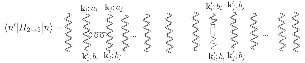
Figure 8: Matrix element given by eq.(80).

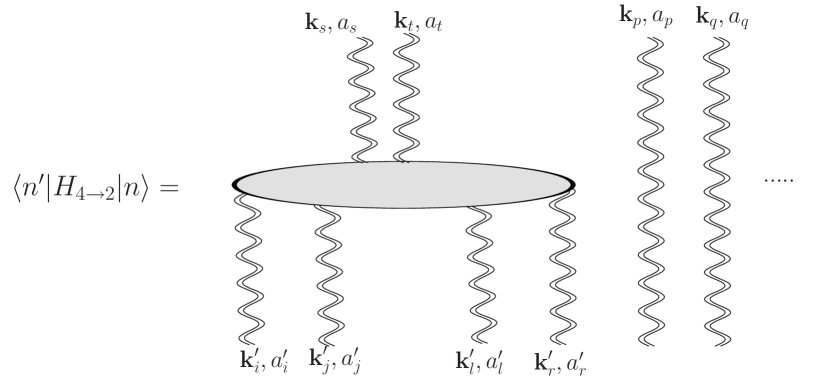
Figure 9: Matrix element given by eq.(81).

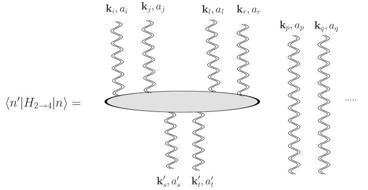
Figure 10: Matrix element given by eq.(82).

In particular, the second term contains the $2\to 4$ transition vertex:

$$\begin{split}\langle n^{\prime}|H_{2\rightarrow 4}|n\rangle=\delta_{n\,n^{\prime}+2}\sum_{s\!>\!t=1}^{n^{\prime}}\sum_{i\!>\!j\!>\!l\!>\!r\!=1}^{n}\bigg{[}{\cal V}^{a_{i}^{\prime}a_{j}^{\prime}a_{l}^{\prime}a_{r}^{\prime};a_{s},a_{t}}(\textbf{k}_{i}^{\prime},\textbf{k}_{j}^{\prime},\textbf{k}_{l}^{\prime},\textbf{k}_{r}^{\prime};\textbf{k}_{s},\textbf{k}_{t})+(\textbf{k}_{s}\leftrightarrow\textbf{k}_{t},a_{s}\leftrightarrow a_{t})\bigg{]}\\ (2\pi)^{3}\delta(\textbf{k}_{i}+\textbf{k}_{j}+\textbf{k}_{l}+\textbf{k}_{r}-\textbf{k}_{i}-\textbf{k}_{j})\frac{1}{(n-4)!}\sum_{\sigma(n-4)}\prod_{p\neq i,j,l,r}^{n}(2\pi)^{3}\delta(\textbf{k}_{p}-\textbf{k}^{\prime}_{p})\delta^{a_{p}a^{\prime}_{p}},\end{split}$$ (81)

whereas the third term allows for four gluon to fuse into two gluons:

$$\begin{split}\langle n^{\prime}|H_{4\rightarrow 2}|n\rangle=\delta_{n\,n^{\prime}-2}\sum_{s\!>\!t}^{n}\!\sum_{i\!>\!j\!>\!l\!>\!r\!=1}^{n^{\prime}}\!\!\!\!\!\bigg{[}{\cal V}^{a_{s}a_{t};a_{i}^{\prime}a_{j}^{\prime}a_{l}^{\prime}a_{r}^{\prime}}(\textbf{k}_{s}^{\prime},\textbf{k}_{t}^{\prime};\textbf{k}_{i},\textbf{k}_{j},\textbf{k}_{l},\textbf{k}_{r})+(\textbf{k}_{s}^{\prime}\leftrightarrow\textbf{k}_{t}^{\prime},a_{s}^{\prime}\leftrightarrow a_{t}^{\prime})\bigg{]}\\ (2\pi)^{3}\delta(\textbf{k}_{i}+\textbf{k}_{j}+\textbf{k}_{l}+\textbf{k}_{r}-\textbf{k}_{s}^{\prime}-\textbf{k}_{t}^{\prime})\frac{1}{(n^{\prime}-4)!}\sum_{\sigma(n^{\prime}-4)}\prod_{p\neq i,j,l,r}^{n^{\prime}}(2\pi)^{3}\delta(\textbf{k}_{p}-\textbf{k}^{\prime}_{p})\delta^{a_{p}a^{\prime}_{p}}.\end{split}$$ (82)

The next two terms on the rhs of (79) belong to the Pomeron $\to$ two Odderon vertex  [22] (restricted to the color singlet channel) and to its inverse, resp. They will not be discussed further. Higher order kernels (indicated by the dots) have not been computed yet. Let us define the $n$ reggeon wave function component of the target at rapidity $y$ in the following way:

$$\psi_{n}^{\{a_{i}\}}(y,\textbf{k}_{1},\textbf{k}_{2}...\textbf{k}_{n})=\langle n|e^{yH}|p\rangle.$$ (83)

Upon differentiation with respect to $y$ we obtain:

$$\frac{\partial\psi^{\{a_{i}\}}_{n}}{\partial y}=\langle n|He^{yH}|p\rangle=\sum_{n^{\prime}}\langle n|H|n^{\prime}\rangle\langle n^{\prime}\!|e^{yH}|\!p\rangle$$

$$=\sum_{n^{\prime}}\langle n|H|\!n^{\prime}\rangle\psi^{\{a_{i}^{\prime}\}}_{n^{\prime}}.$$ (84)

This defines an infinite set of coupled equations. It cannot be closed because, for instance, the equation for the two gluon wave function receives contributions coming from the four gluon wave function:

$$\frac{\partial\psi^{a_{1}a_{2}}_{2}}{\partial y}=\langle 2|H_{2\rightarrow 2}|2\rangle\psi_{2}^{a_{1}a_{2}}-\langle 2|H_{4\rightarrow 2}|4\rangle\psi_{4}^{a_{1}a_{2}}$$ (85)

(the term proportional to (81) vanishes since it requires zero gluons in the initial state).

6.2 The nonlinear equation for the unintegrated gluon density

In order to reach further simplification, we take the large-$N_{c}$ limit. In practice this implies that we group the $n$ gluons into $n/2$ color singlet pairs (Pomerons) and associate with each pair a color singlet projector: this projector acts on the color tensors of the interaction Hamiltonians and leads to color weight factors of the interaction kernels. In particular, in the $2\to 2$ Hamiltonian the color tensor $f_{a_{i}a_{i}^{\prime}c}f_{ca_{j}^{\prime}a_{j}}$ is replaced by the color factor $-N_{c}$, and in the $2\to 4$ Hamiltonian, $H_{2\to 4}$, the $2\to 4$ vertex ${\cal V}^{a_{s}a_{t};a_{i}^{\prime}a_{j}^{\prime}a_{m}^{\prime}a_{n}^{\prime}}$ reduces to the function $V(\textbf{k}_{i}^{\prime},\textbf{k}_{j}^{\prime},\textbf{k}_{m}^{\prime},\textbf{k}_{n}^{\prime})$ (cf. eq.(1)). The evolution equations have to be reformulated in terms of $N$ states of gluon pairs: each pair carries two momentum variables, q and k: q denotes the total tranverse momentum of the two gluon state, and k, $\textbf{q}-\textbf{k}$ are the momenta of the two constituent gluons. The state consisting of $N=n/2$ such pairs is defined as:

$$|N\rangle = \frac{1}{\sqrt{N!}}A^{\dagger}(\textbf{q}_{1},\textbf{k}_{1})...A^{\dagger}(\textbf{q}_{N},\textbf{k}_{N})|0\rangle$$ (86)

$$= |(\textbf{q}_{1},\textbf{k}_{1}),..(\textbf{q}_{N},\textbf{k}_{N})\rangle$$

(we use capital letters to distinguish the pair-basis from the reggeon basis). The normalization follows from

$$[A(\textbf{q},\textbf{k}),A^{\dagger}(\textbf{q}^{\prime},\textbf{k}^{\prime})]=(2\pi)^{6}\textbf{k}^{2}(\textbf{q}-\textbf{k})^{2}\delta(\textbf{q}-\textbf{q}^{\prime})\delta(\textbf{k}-\textbf{k}^{\prime}),$$ (87)

in analogy with the reggeon states. We write the Hamiltonian as

$$H=H_{1\to 1}+H_{1\to 2}+H_{2\to 1},$$ (88)

where

$$\langle 1|H_{1\to 1}|1\rangle=N_{c}\bigg{\{}K_{2\to 2}(\textbf{k}_{i},\textbf{k}_{j};\textbf{k}_{i}^{\prime},\textbf{k}_{j}^{\prime})(2\pi)^{3}\delta(\textbf{k}_{i}+\textbf{k}_{j}-\textbf{k}_{i}^{\prime}-\textbf{k}_{j}^{\prime})$$

$$+\left(\omega(\textbf{k}_{i})+\omega(\textbf{k}_{j})\right)\textbf{k}_{i}^{2}\textbf{k}_{j}^{2}\delta(\textbf{k}_{i}-\textbf{k}_{i}^{\prime})\delta(\textbf{k}_{j}-\textbf{k}_{j}^{\prime})\bigg{\}}+(\textbf{k}_{i}^{\prime}\leftrightarrow\textbf{k}_{j}^{\prime})$$ (89)

and

$$\langle 1|H_{1\to 2}|2\rangle=\bigg{[}V(\textbf{k}_{i}^{\prime},\textbf{k}_{j}^{\prime},\textbf{k}_{l}^{\prime},\textbf{k}_{r}^{\prime};\textbf{k}_{s},\textbf{k}_{t})+(\textbf{k}_{s}\leftrightarrow\textbf{k}_{t},a_{s}\leftrightarrow a_{t})\bigg{]}$$ (90)

$$(2\pi)^{3}\delta(\textbf{k}_{i}+\textbf{k}_{j}+\textbf{k}_{l}+\textbf{k}_{r}-\textbf{k}_{i}-\textbf{k}_{j}).$$ (91)

The amplitudes $\Psi_{N}$ in this basis of gluon pairs are defined in analogy with (83).

Next we invoke the mean field approximation and make the following factorizing ansatz:

$$\Psi_{2}(y,\textbf{k}_{1},\textbf{q}_{1}-\textbf{k}_{1},\textbf{k}_{2},\textbf{q}_{2}-\textbf{k}_{2})=\Psi_{1}(y,\textbf{k}_{1},\textbf{q}_{1}-\textbf{k}_{1})\Psi_{1}(y,\textbf{k}_{2},\textbf{q}_{2}-\textbf{k}_{2}).$$ (92)

This ansatz can be justified for a large nuclear target. It allows to obtain a closed equation for $\Psi_{1}$:

$$\frac{\partial\Psi_{1}}{\partial y}=\langle 1|H_{1\rightarrow 1}|1\rangle\Psi_{1}-\frac{1}{\sqrt{2}}\langle 1|H_{2\rightarrow 1}|2\rangle\Psi_{1}\Psi_{1}.$$ (93)

To obtain the BK equation for the unintegrated gluon density let us define the off-diagonal unintegrated gluon density via:

$${\cal F}(y,\textbf{k}_{1},\textbf{k}_{2})=\Psi_{1}(y,\textbf{k}_{1},\textbf{k}_{2})=\langle 1|e^{-yH}|p\rangle.$$ (94)

Using (80), (81), (89), (93), (94) we obtain the nonlinear evolution equation:

$$\begin{split}\frac{\partial{\cal F}(x,\textbf{q},\textbf{k})}{\partial\ln 1/x}=\!\!\int\!\!\frac{d^{2}\textbf{l}}{(2\pi)^{3}}K(\textbf{l},\textbf{q}-\textbf{l};\textbf{k},\textbf{q}-\textbf{k})\frac{{\cal F}(x,\textbf{q},\textbf{l})}{\textbf{l}^{2}(\textbf{q}-\textbf{l})^{2}}\\ \end{split}$$

$$\begin{split}-\pi\int d^{2}\textbf{r}\frac{d^{2}\textbf{l}}{(2\pi)^{3}}\frac{d^{2}\textbf{m}}{(2\pi)^{3}}V(\textbf{k},-\textbf{k}+\textbf{q};\textbf{l},-\textbf{l}-\frac{\textbf{q}}{2}+\textbf{r},\textbf{m},-\textbf{m}-\frac{\textbf{q}}{2}-\textbf{r})\\ \times\frac{{\cal F}(x,\frac{\textbf{q}}{2}+\textbf{r},\textbf{l})}{\textbf{l}^{2}(-\textbf{l}+\frac{\textbf{q}}{2}+\textbf{r})^{2}}\frac{{\cal F}(x,\frac{\textbf{q}}{2}-\textbf{r},\textbf{m})}{\textbf{m}^{2}(-\textbf{m}+\frac{\textbf{q}}{2}-\textbf{r})^{2}}.\end{split}$$ (95)

The momenta entering the vertex from below are labeled by $\textbf{k}_{1}^{\prime}\!\!=\!\!\textbf{l}$, $\textbf{k}_{2}^{\prime}\!\!=\!\!-\textbf{l}\!-\!\textbf{q}/2+\textbf{r}$, $\textbf{k}_{3}^{\prime}\!\!=\!\!\textbf{m}$, $\textbf{k}_{4}^{\prime}\!\!=\!\!-\textbf{m}-\textbf{q}/2-\textbf{r}$. The variable r stands for the loop momentum. In  [11] it has been shown that this equation coincides with the Balitsky-Kovchegov equation, provided the solutions ${\cal F}$ belong to the Möbius class of functions (i.e. the Fourier transform vanishes when the two coordinates become identical). We make the assumption that the coupling to the proton goes via the form factor (with momentum transfer r)

$$F(\textbf{r},R)=\frac{e^{\frac{-\textbf{r}^{2}R^{2}}{4}}}{2\pi},$$ (96)

(where $R$ has the meaning of the proton radius), and for ${\cal F}(x,\textbf{r},\textbf{k})$ we make the ansatz:

$${\cal F}(x,\textbf{r},\textbf{k})={\cal F}(x,\textbf{k})F(\textbf{r},R).$$ (97)

Then the integration over r on the rhs of (95) will be restricted to small values $\textbf{r}^{2}\leq 1/R^{2}$. Now we restrict ourselves to zero momentum transfer, $\textbf{q}=0$, which corresponds to the integration over the impact parameter, and, as further approximation, we put $\textbf{r}=0$ at the TPV: in the dipole language, this means that the typical dipole size is assumed to be much smaller than the impact parameter $b$. This allows to carry out the r integral, and one easily sees that the function ${\cal F}(x,\textbf{k})$ satisfies the somewhat simpler equation:

$$\begin{split}\frac{\partial{\cal F}(x,\textbf{k})}{\partial\ln 1/x}=\int\frac{d^{2}\textbf{l}}{(2\pi)^{3}}K(\textbf{l},-\textbf{l};\textbf{k},-\textbf{k})\frac{{\cal F}(x,\textbf{l})}{\textbf{l}^{4}}\\ -\pi\frac{1}{2\pi R^{2}}\int\frac{d^{2}\textbf{l}}{(2\pi)^{3}}\frac{d^{2}\textbf{m}}{(2\pi)^{3}}V(\textbf{k},-\textbf{k};\textbf{l},-\textbf{l},\textbf{m},-\textbf{m})\frac{{\cal F}(x,\textbf{l})}{\textbf{l}^{4}}\frac{{\cal F}(x,\textbf{m})}{\textbf{m}^{4}}.\end{split}$$ (98)

In the next step we perform the integrations over the azimuthal angles of l, m, and k. Denoting the integrated function ${\cal F}(x,\textbf{k})$ by $f(x,\textbf{k}^{2})$:

$$f(x,\textbf{k}^{2})=\frac{1}{2\pi}\int\!d\phi{\cal F}(x,\textbf{k})$$ (99)

with

$$xg(x,\textbf{k}^{2})=\int^{\textbf{k}^{2}}\frac{d\textbf{k}^{\prime 2}}{\textbf{k}^{\prime 2}}f(x,\textbf{k}^{\prime 2}),$$ (100)

and using our result (51) for the angular averaged TPV, the nonlinear equation reads[8, 9]:

$$\begin{split}\frac{\partial f(x,\textbf{k}^{2})}{\partial\ln 1/x}=\frac{N_{c}\alpha_{s}}{\pi}\textbf{k}^{2}\int_{0}^{\infty}\frac{d\textbf{l}^{2}}{\textbf{l}^{2}}\bigg{[}\frac{f(x,\textbf{l}^{2})-f(x,\textbf{k}^{2})}{|\textbf{k}^{2}-\textbf{l}^{2}|}+\frac{f(x,\textbf{k}^{2})}{\sqrt{(4\textbf{l}^{4}+\textbf{k}^{4})}}\bigg{]}\\ -\frac{\alpha_{s}^{2}}{2R^{2}}\Bigg{\{}2\textbf{k}^{2}\bigg{[}\int_{\textbf{k}^{2}}^{\infty}\frac{d\textbf{l}^{2}}{\textbf{l}^{4}}f(x,\textbf{l}^{2})\bigg{]}^{2}+2\;f(x,\textbf{k}^{2})\int_{\textbf{k}^{2}}^{\infty}\frac{d\textbf{l}^{2}}{\textbf{l}^{4}}\ln\left(\frac{\textbf{l}^{2}}{\textbf{k}^{2}}\right)f(x,\textbf{l}^{2})\Bigg{\}}.\end{split}$$ (101)

When applying this equation to the scattering of a virtual photon on a nucleus we return to the question raised at the end of the introduction, the question of the most dominant gluon configurations. In the DGLAP approach one has strong ordering in momentum, i.e virtualities of gluons closer to photon are larger than those closer to the target. In the nonlinear evolution equation one then would expect that, at the kernel of the nonlinear term, the upper momenta, $k$, should be larger than the lower ones, $\textbf{l}^{2}$ and $\textbf{m}^{2}$. However, making use of our results for the collinear limit of the TVP and of the structure of the angular averaged vertex, we arrive at the somewhat surprising conclusion that the momenta are ordered in the opposite direction. In more physical terms, the recombination of two smaller gluons ends up in a larger gluon. This suppression of softer gluons below the nonlinear term may explain why, in numerical solutions of the angular averaged BK equation for the unintegrated gluon  [9], the BFKL diffusion into the infrared region is absent.

7 Comparison with other equations

As we have mentioned before, the nonlinear equation (95) coincides with the Balitsky-Kovchegov equation. In  [11], the Fourier transform of (95) has been computed, and it has been shown that, in the class of Möbius functions, it agrees with the BK equation.

Alternatively, one can start  [8, 9, 10] from the Balitsky-Kovchegov equation for the dipole scattering amplitude in coordinate space, and compute the Fourier transform to momentum space. The connection between the momentum space gluon distribution ${\cal F}(x,\textbf{q},\textbf{k})$ and the dipole scattering amplitude is:

$${\cal F}(x,\textbf{q},\textbf{k})=\frac{N_{c}}{4\alpha_{s}\pi^{2}}\textbf{k}^{2}(\textbf{k}-\textbf{q})^{2}\nabla^{2}_{k}\int\frac{d^{2}\textbf{x}_{0}}{2\pi}\int\frac{d^{2}\textbf{x}_{1}}{2\pi}e^{i\textbf{k}\cdot\textbf{x}_{0}}e^{i(\textbf{q}-\textbf{k})\cdot\textbf{x}_{1}}\frac{N(\textbf{x}_{01},\textbf{b},x)}{\textbf{x}_{01}^{2}},$$ (102)

where $\textbf{x}_{01}\!=\!\textbf{x}_{0}-\textbf{x}_{1}$, and $\textbf{b}\!=\!(\textbf{x}_{1}+\textbf{x}_{2})/2$ is the impact parameter. Our steps of approximation described after (95) are equivalent to the factorization ansatz

$$N({\textbf{x}_{01}},{\bf b},x)=N(\textbf{x}_{01},x)S(\textbf{b})$$ (103)

and to the assumption that, in the Balitsky-Kovchegov equation, all dipole sizes are much smaller than the impact parameter $b$. With these approximations one arrives, after angular averaging and integration over impact parameter $b$, at the nonlinear equation (101).

Returning, once more, to the issue of the twist expansion, we have to conclude that the nonlinear BK equation, when restricting to solutions with conformal spin $n=0$, receives all its contributions from ’anticollinear’ terms. This, in connection with corrections to the single-ladder approximation at small $x$, makes the usefulness of a twist expansion some what doubtful.

Let us finally comment on other versions of nonlinear evolution equations. The first nonlinear evolution equation which was a milestone in physics of saturation is the Gribov-Levin-Ryskin, Mueller-Qiu (GLR-MQ) equation [25], [26] (eqn(2.41) in [25], and eqn.(30) in [26]), obtained in the double-logarithmic approximation:

$$\frac{\partial^{2}xg(x,\textbf{k}^{2})}{\partial\ln(1/x)\partial\ln\textbf{k}^{2}}=\frac{\alpha_{s}N_{c}}{\pi}xg(x,\textbf{k}^{2})-C\frac{\alpha_{s}^{2}}{\textbf{k}^{2}R^{2}}[xg(x,\textbf{k}^{2})]^{2}.$$ (104)

(the constant C is not the same in the two papers; however, for our discussion this is not essential). This equation can be rewritten in terms of the unintegrated gluon density $f(x,\textbf{k}^{2})$:

$$\frac{\partial f(x,\textbf{k}^{2})}{\partial\ln 1/x}=\frac{N_{c}\alpha_{s}}{\pi}\int_{k_{0}^{2}}^{\textbf{k}^{2}}\frac{d\textbf{l}^{2}}{\textbf{l}^{2}}f(x,\textbf{l}^{2})-C\frac{\alpha_{s}^{2}}{\textbf{k}^{2}R^{2}}\bigg{[}\int_{\textbf{k}_{0}^{2}}^{\textbf{k}^{2}}\frac{d\textbf{l}^{2}}{\textbf{l}^{2}}f(x,\textbf{l}^{2})\bigg{]}^{2}$$ (105)

The linear term coincides with the BFKL kernel in the collinear approximation. The nonlinear term should be interpreted as the TPV at the collinear limit. Its physical interpretation would support the strong ordering (collinear) picture discussed at the end of the previous section: momenta above ($k^{2}$) are larger than below (${k^{\prime}}^{2}$) the nonlinear interaction. Our analysis, however, does not agree with this form of the nonlinear term. The structure of integrals is totally different. In particular, we have come to the conclusion that, after angular averaging, the TPV does not contribute to the collinear limit.

The GLR paper [25] also presents another nonlinear equation (eq.(2.108)), derived from summing up, at small $x$, single logs of the fan diagrams. It is written directly for the unintegrated gluon density which, in the GLR notation, differs from our definition (eq.(100):

$$xg(x,\textbf{k}^{2})=\int^{k^{2}}\!\!\!d\textbf{k}^{\prime 2}\Phi(x,\textbf{k}^{\prime 2}).$$ (106)

This equation is an attempt to generalize the BFKL equation to the physics of dense systems, and its form is quite close to our equation (101):

$$\frac{\partial\Phi(x,\textbf{k}^{2})}{\partial\ln 1/x}=\frac{N_{c}\alpha_{s}}{\pi}\int^{\infty}_{0}\frac{d\textbf{l}^{2}}{\textbf{l}^{2}}\left[\frac{\Phi(x,\textbf{l}^{2})-\Phi(x,\textbf{k}^{2})}{|\textbf{l}^{2}-\textbf{k}^{2}|}-\frac{\Phi(x,\textbf{k}^{2})}{\sqrt{4\textbf{l}^{4}+\textbf{k}^{4}}}\right]-g_{TPV}\frac{1}{4\pi R^{2}}\left(\frac{\alpha_{s}}{4\pi}\right)^{2}\Phi^{2}(x,\textbf{k}^{2}),$$ (107)

where $g_{TPV}$ is the local approximation of the following TPV vertex:

$$V\otimes\left(\Phi(x,\textbf{l}^{2})\Phi(x,\textbf{m}^{2})\right)=\int\frac{d\textbf{m}^{2}}{\textbf{l}^{2}}\frac{d\textbf{l}^{2}}{\textbf{l}^{2}}\alpha_{s}(\textbf{m}^{2})\alpha_{s}(\textbf{l}^{2})\Phi(x,\textbf{m}^{2})\Phi(x,\textbf{l}^{2})\theta(\textbf{l}^{2}-\textbf{k}^{2})\theta(\textbf{m}^{2}-\textbf{k}^{2}).$$ (108)

This vertex contains the same $\theta$-functions as in (51), and it thus supports the physical picture describes at the end of the previous section. On the other hand, the detailed analytic form of the vertex is different from (101); in particular, it does not contain the disconnected pieces which, in the original derivation of the $2\to 4$ vertex, can be traced back to the reggeization of the gluon (there are also differences in the prefactors).

Despite these differences in the detailed form of the nonlinear equations it may very well be that, as far as the gross features of saturation are concerned, the qualitative behavior of solutions will be similar. It would be interesting to study this in more detail.

8 Conclusions

In this paper we have investigated the momentum space triple Pomeron vertex. In particular, we have studied its collinear and anticollinear limits. This question arises naturally if one studies nonlinear corrections to the linear BFKL evolution in deep inelastic scattering at small $x$: one expects that, at least on the average, transverse momenta decrease when moving from the photon to the proton. In a first step one is then led to consider the limit of strong ordering. Restricting ouselves to solutions with conformal spin zero, we have shown, for the simplest example of a fan diagram with one triple Pomeron vertex in the large-$N_{c}$ limit, that there is no contribution from the configuration of strongly ordered gluons. Beyond the large-$N_{c}$ limit such contributions exist.

We have also constructed a set of evolution equations for the interaction of a photon with a nuclear target, which, in the mean field approximation, reduces to a nonlinear evolution equation for the skewed unintegrated gluon density which, in the forward region, agrees with equation obtained in [8, 9]. We have also compared our momentum space expression for the nonlinear evolution kernel with different other versions discussed in the literature. We agree with the BK equation, but we find disagreement with other earlier versions of nonlinear evolution equations.

Interpretating our results in terms of twist, we have shown that the BK-equation, when restricted to solutions with conformal spin zero, receives all its contributions from ’anticollinear’ configurations, quite in contrast to the expected ordering of transverse momenta.

We also hope that our analysis will help to analyse further the contributions of pomeron loops.

References

- [1] J. Bartels, Z. Phys. C 60 (1993) 471-488.
- [2] J. Bartels, M. Wusthoff, Z. Phys. C 66 (1995) 157.
- [3] I. I. Balitsky, Nucl. Phys. B463 (1996) 99; in *Shifman, M. (ed.): At the frontier of particle physics, vol. 2* 1237-1342. e-Print: hep-ph/0101042.
- [4] I. I. Balitsky, Phys. Rev. Lett. 81 (1998) 2024; Phys. Rev. D60 (1999) 014020; itPhys. Lett. B518 (2001) 235;
- [5] Yu. V. Kovchegov, Phys.Rev D60 (1999) 034008
-
[6]
E. Iancu, D. N. Triantafyllopoulos, Nucl. Phys. A756 (2005) 419-467,
J.-P. Blaizot, E. Iancu, K. Itakura, D.N. Triantafyllopoulos, Phys.Lett. B615 (2005) 253-261,
A. Kovner, M. Lublinsky, Nucl.Phys A767 171-188,2006,
A. Kovner, M. Lublinsky, Phys. Rev. D71 (2005) 085004 - [7] J. Bartels, M.G. Ryskin, G.P. Vacca, Eur. Phys. J.C 27 (2003) 101
- [8] M.A. Kimber, J. Kwieciński and A.D. Martin, Phys. Lett. B 508 (2001) 58.
- [9] K. Kutak and J. Kwieciński, Eur. Phys. J.C 29 (2003) 521.
- [10] K. Kutak and A.M. Staśto, Eur. Phys. J.C 41 (2005) 343
- [11] J. Bartels, L. Lipatov, J. P. Vacca, Nucl.Phys. B 706 (2005) 391-410
- [12] J. Bartels, L. Lipatov, M. Wüsthoff, Nucl.Phys. B464 (1996) 298-318
- [13] M. Braun, J. P. Vacca, Eur. Phys. J.C 6 (1999) 147.
- [14] V.A. Abramovski,V.N. Gribov,O. V. Kanchelli, Sov. Journ. Nucl. Phys. 18 (1973) 595
- [15] J. Bartels, J.P. Vacca, M. Salvadore, Eur. Phys. J.C 42 (2005) 53.
- [16] J. P. Vacca, PhD Thesis arXiv:hep-ph/9803283
-
[17]
L. N. Lipatov, Sov. J. Nucl. Phys.
23 (1976) 338;
E. A. Kuraev, L. N. Lipatov and V. S. Fadin, Sov. Phys. JETP 45 (1977) 199;
I. I. Balitsky and L. N. Lipatov, Sov. J. Nucl. Phys. 28 (1978) 338. - [18] J. Bartels, Nucl. Phys. B175 (1980) 365.
- [19] J. Kwieciński, M. Praszalowicz, Phys. Lett B94 (1980) 413.
- [20] N. N. Nikolaev, B. G. Zakharov, Z. Phys.C 53 (1992) 331
- [21] A.H. Mueller, Nucl.Phys. B335 (1990) 115
- [22] J. Bartels, C. Ewerz, JHEP 9909 (1999) 026
- [23] J. Bartels, M. Ryskin, J. P. Vacca, Eur.Phys.J. C27 (2003) 101-113
- [24] M. Braun, Eur.Phys.J. C16 (2000) 337-347
- [25] L. V. Gribov, E. M. Levin and M. G. Ryskin, Phys. Rep. 100 (1983) 1.
- [26] A. H. Mueller, J. W. Qiu, Nucl. Phys B 268 427 (1986)