How we discovered
the nonet of light scalar mesons

Abstract

As has been confirmed meanwhile by lattice-QCD calculations (see e.g. Ref. [1]), the confinement spectrum of non-exotic quark-antiquark systems has its ground state for scalar mesons well above 1 GeV in the Resonance Spectrum Expansion (RSE). For instance, in the $S$-wave $K\pi$ RSE amplitude, a broad resonance was predicted slightly above 1.4 GeV [2], which is confirmed by experiment as the $K^{\ast}_{0}$(1430). However, a complete nonet of light scalar mesons was predicted [3] as well, when a model strongly related to the RSE and initially developed to describe the $c\bar{c}$ and $b\bar{b}$ resonance spectra [4] was applied in the light-quark sector. Thus, it was found that the light scalar-meson nonet constitutes part of the ordinary meson spectrum, albeit represented by “extraordinary” [5] poles [2]. Similar resonances and bound states appear in the charmed sector [6], and are predicted in the $B$-meson spectrum [7, 8].

A recent work [9] confirmed the presence of light scalar-meson poles in the RSE amplitude for $S$-wave and $P$-wave $\pi\pi$ and $K\pi$ contributions to three-body decay processes measured by the BES, E791 and FOCUS collaborations.

1 Scattering poles

It is generally accepted that resonances in scattering are represented by poles in the “second” Riemann sheet of the complex energy plane [10]. Let us assume here that in a process of elastic and non-exotic meson-meson scattering one obtains scattering poles at

$$E\;=\;P_{0}\,,\;\;P_{1}\,,\;\;P_{2}\,,\;\;\dots\;\;\;.$$ (1)

Simple poles in $S$ may be considered simple zeros in its denominator. Hence, assuming a polynomial expansion, we may [11, 12] represent the denominator $D$ of $S$ by

$$D(E)\;\propto\;\left(E-P_{0}\right)\left(E-P_{1}\right)\left(E-P_{2}\right)\dots\;\;\;.$$ (2)

Unitarity then requires that the $S$-matrix be given by

$$S(E)\;=\;\frac{\textstyle\raisebox{5.0pt}{ $\left(E-P_{0}^{\ast}\right)\left(E-P_{1}^{\ast}\right)\left(E-P_{2}^{\ast}\right)\dots$}}{\textstyle\raisebox{-5.0pt}{ $\left(E-P_{0}\right)\left(E-P_{1}\right)\left(E-P_{2}\right)\dots$}}\;\;\;.$$ (3)

If we assume that the resonances (1) stem from an underlying confinement spectrum, given by the real quantities

$$E\;=\;E_{0}\,,\;\;E_{1}\,,\;\;E_{2}\,,\;\;\dots\;\;\;,$$ (4)

then we may represent the differences $\left(P_{n}-E_{n}\right)$, for $n=0$, 1, 2, $\dots$, by $\Delta E_{n}$. Thus, we obtain for the unitary $S$-matrix the expression

$$S(E)\;=\;\frac{\textstyle\raisebox{5.0pt}{$\left(E-E_{0}-{\Delta E_{0}}^{\ast}\right)\left(E-E_{1}-{\Delta E_{1}}^{\ast}\right)\left(E-E_{2}-{\Delta E_{2}}^{\ast}\right)\dots$}}{\textstyle\raisebox{-5.0pt}{$\left(E-E_{0}-\Delta E_{0}\right)\left(E-E_{1}-\Delta E_{1}\right)\left(E-E_{2}-\Delta E_{2}\right)\dots$}}\;\;\;.$$ (5)

So we assume here that resonances occur in scattering because the two-meson system couples to confined states, usually of the $q\bar{q}$ type, viz. in non-exotic meson-meson scattering. Let the strength of the coupling be given by $\lambda$. For vanishing $\lambda$, we presume that the widths and real shifts of the resonances also vanish (see Fig. 1). Consequently, the scattering poles end up at the positions of the confinement spectrum (4), and so

$$\Delta E_{n}\;\begin{array}[]{c}\\ \longrightarrow\\ \lambda\!\!\downarrow\!0\end{array}\;0\;\;\;\;{\textstyle\mbox{\rm for}}\;\;\;\;n\;=\;0,\;\;1,\;\;2,\;\;\dots\;\;\;.$$ (6)

As a result, the scattering matrix tends to unity, as expected in case there is no interaction.

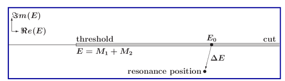
Figure 1: Illustration of a scattering pole and the related energy level $E_{0}$ of the confinement spectrum (4).

An obvious candidate for an expression of the form (5) looks like

$$S(E)\;=\;\frac{\textstyle\raisebox{10.0pt}{$1+\lambda^{2}\,\left\{{\displaystyle\sum_{n}}\frac{\textstyle G(E)^{\ast}}{\textstyle E-E_{n}}\right\}$}}{\textstyle\raisebox{-10.0pt}{$1+\lambda^{2}\,\left\{{\displaystyle\sum_{n}}\frac{\textstyle G(E)}{\textstyle E-E_{n}}\right\}$}}\;\;\;,$$ (7)

where $G$ is a smooth complex function of energy $E$, and where, at least for small values of the coupling constant $\lambda$, one has

$$\Delta E_{i}\;\approx\;-\lambda^{2}\,G\left(E_{i}\right)\;\;\;\;{\textstyle\mbox{\rm for}}\;\;\;\;i\;=\;0,\;\;1,\;\;2,\;\;\dots\;\;\;.$$ (8)

Relation (8) can be easily understood, if we assume that for small $\lambda$ poles show up in the vicinity of the energy values (4) of the confinement spectrum. As a consequence, at the zero $P_{i}$ of the denominator, near the $i$-th recurrency of the confinement spectrum $E_{i}$, the term $n=i$ dominates the summations in formula (7), i.e.,

$$0\;=\;1+\lambda^{2}\,\left\{{\displaystyle\sum_{n}}\frac{\textstyle G\left(P_{i}\right)}{\textstyle P_{i}-E_{n}}\right\}\;\approx\;1+\lambda^{2}\,\frac{\textstyle G\left(E_{i}\right)}{\textstyle\Delta E_{i}}\;\;\;.$$ (9)

For larger values of $\lambda$, one cannot perform the approximation $P_{i}\approx E_{i}$ in Eq. (9). In such cases, the left-hand part of Eq. (9) must be solved by other methods, usually numerically. However, since it is reasonable to assume that poles move smoothly in the lower half of the complex energy plane as $\lambda$ varies, we may suppose that the left-hand part of Eq. (9) has solutions which, when the value of $\lambda^{2}$ is continuously decreased, each correspond to one of the values out of the confinement spectrum (4).

When all scattering poles in expression (5) are known, one can — with unlimited accuracy — determine the function $G$ in formula (7). Once $G$ is known, one can search for poles by solving the left-hand part of Eq. (9). However, further restrictions can be imposed upon expression (7). For a two-meson system, there may exist bound states below the meson-meson scattering threshold. Such states are represented by poles in the analytic continuation of expression (7) to below threshold, on the real axis in the complex energy plane. Consequently, in the case that a confinement state, say $E_{0}$, comes out below threshold, its corresponding pole is, at least for small coupling, expected to be found on the real axis in the complex energy plane. Using formula (8), we obtain

$$G\left(E_{0}\right)\;\;{\textstyle\mbox{\rm real}}\;\;\;\;{\textstyle\mbox{\rm for}}\;\;\;\;E_{0}\,<\,{\textstyle\mbox{\rm threshold.}}$$ (10)

Moreover, in order to ensure that scattering poles come out in the lower-half of the complex energy plane, also using formula (8), we find that above threshold $G$ must be complex, with a positive imaginary part.

2 Partial waves

In different partial waves, resonances come out at different masses. At threshold, where the total invariant mass of the two-meson system equals the sum of the two meson masses, one has additional conditions. For $S$ waves, since cross sections are finite, we must demand that $G$ do not vanish at threshold, whereas, for $P$ and higher waves, as cross sections do vanish, $G$ should vanish as well.

A possible expression that satisfies all imposed conditions reads

$$i\,pa\,j_{\ell}(pa)\,h^{(1)}_{\ell}(pa)\;\;\;\;{\textstyle\mbox{\rm for}}\;\;\;\;\ell\;=\;0,\;\;1,\;\;2,\;\;\dots\;\;\;,$$ (11)

where $p$ represents the linear momentum in the two-meson system and $a$ a scale parameter with the dimensions of a distance. The well-known scattering solutions $j_{\ell}$ and $h^{(1)}_{\ell}$ stand for the spherical Bessel function and the Hankel function of the first kind, respectively.

Thus, we arrive at a good candidate for a scattering amplitude of resonant scattering off a confinement spectrum, reading

$$T_{\ell}(E)\;=\;\frac{1}{2i}\left(S_{\ell}(E)-1\right)\;=\;\frac{\textstyle\raisebox{12.0pt}{$-2\lambda^{2}\,\left\{{\displaystyle\sum_{n}}\frac{\textstyle\raisebox{5.0pt}{$g_{n\ell}^{2}$}}{\textstyle\raisebox{-5.0pt}{$E-E_{n}$}}\right\}\,\mu pa\,j^{2}_{\ell}(pa)$}}{\textstyle\raisebox{-12.0pt}{$1+2i\lambda^{2}\,\left\{{\displaystyle\sum_{n}}\frac{\textstyle\raisebox{5.0pt}{$g_{n\ell}^{2}$}}{\textstyle\raisebox{-5.0pt}{$E-E_{n}$}}\right\}\,\mu pa\,j_{\ell}(pa)\,h^{(1)}_{\ell}(pa)$}}\;,$$ (12)

where we have introduced the two-meson reduced mass $\mu$ and, moreover, relative couplings $g_{n\ell}$, which may be different for different recurrencies of the confinement spectrum.

As it is written, formula (12) seems to allow a lot of freedom, through adjustments of the $g_{n\ell}$ to experiment. In principle, it might even be useful to carry out such data fitting, so as to gain more insight into the details of the coupling between a two-meson system and a confined $q\bar{q}$ state. However, experimental results are so far much too incomplete to make a detailed comparison to our expression possible.

The spin structure of quarks, besides being important for the spectrum of a $q\bar{q}$ system, is also crucial for the short-distance dynamics, hence for the properties of the coupling between $q\bar{q}$ and meson-meson states. In the ${}^{3\!}P_{0}$ model [13, 14], it is assumed that a two-meson system couples to a $q\bar{q}$ state via the creation or annihilation of a new $q\bar{q}$ pair, with vacuum quantum numbers $J^{PC}=0^{++}$. Under this assumption, all relative couplings can be determined from convolution integrals of the wave functions. In Refs. [15, 16], such integrals have been calculated for general quantum numbers, including flavour. The latter results leave no freedom for the coupling constants in formula (12), except for an overall strength $\lambda$, which parametrises the probability of $q\bar{q}$ creation/annihilation.

This way, the full spin structure of the two-meson system is entirely contained in the relative coupling constants $g_{n\ell}$. Yet, direct comparison of the results given in Refs. [15, 16] to experiment would still be of great interest.

The relevant $q\bar{q}\leftrightarrow MM$ coupling-constant book-keeping has been developed in Refs. [15, 16]. The latter scheme not only eliminates any freedom, but also — by construction — restricts the number of possible $MM$ channels that couple to a given $q\bar{q}$ system. Nonetheless, the number of involved channels rapidly grows for higher radial and angular excitations of the $q\bar{q}$ system.

3 Observables

The scattering matrix is not directly observable, but only through quantities like cross sections and production rates. It is straightforward to determine cross sections [17] and, after some algebra, production rates [18] from expression (12). However, a complete modelling of strong interactions is more complex. For example, a $c\bar{c}$ vector state couples, via OZI-allowed decay, to $D\bar{D}$, but also to $DD^{\ast}$, $D^{\ast}D^{\ast}$, $D_{s}\bar{D}_{s}$, … [4]. Consequently, the involved two-meson channels couple to one another as well. So the first extension necessary for a more proper description of strong interactions is the formulation of a multichannel equivalent of expression (12). This issue has been dealt with in Ref. [19]. It involves coupling constants similar to the ones discussed above, but now for each two-meson channel.

A meson-meson channel is characterised by quantum numbers, including flavour and isospin, and the meson masses. However, many of the needed masses are unknown yet, while most mesons only exist as resonances.

In experiment, one can concentrate on one specific channel. On the other hand, in a meaningful analysis all channels that couple must be taken into account. For example, one may argue that for the description of $\pi\pi$ scattering below the $KK$ threshold the channels $KK$, $\eta\eta$, … can be neglected. But then one ignores virtual two-meson channels, which may have a noticeable influence below the $KK$ threshold.

Furthermore, $q\bar{q}$ states may couple to one another via meson loops. Typical examples are: $c\bar{c}$ vector states, which become mixtures of ${}^{3\!}S_{1}$ and ${}^{3\!}D_{1}$ via loops of charmed mesons, and isoscalar $q\bar{q}$ states, where kaon loops mix the $u\bar{u}+d\bar{d}$ and $s\bar{s}$ components. One then obtains different interplaying confinement spectra, which may become visible in production rates. The extension of expression (7) to more than one $q\bar{q}$ channel has been considered in Refs. [3, 20], for the description of the $\sigma$ and $f_{0}$(980) resonances.

4 The parameters

Besides the parameters $\lambda$ and $a$, formula (12) contains an infinite number of parameters $E_{n\ell}$. These represent the unknown and even hypothetical spectra of confined $q\bar{q}$ systems. From experiment, we only have data at our disposal for resonances in meson-meson scattering or production. Formulae like expression (12) are intended to interpolate between the observed resonances and the underlying — largely unknown — confinement spectrum.

In Fig. 2 of Ref. [21] (see Fig. 3), we showed, for $S$-wave isodoublet $K\pi$ scattering, how cross sections determined by the use of formula (12) vary with increasing values of the coupling $\lambda$. For small $\lambda$, the nonstrange-strange ($n\bar{s}$) confinement spectrum is well visible in the latter figure, whereas for the model value of the $q\bar{q}\,\leftrightarrow$ meson-meson coupling experiment is reproduced.

Figure 2: The theoretical values of the central resonance positions for charmonium S and D states for various values of the model parameter $\lambda$, compared to the experimental situation. The various dashed lines indicate the threshold positions of the strong decay channels DD, DD^∗, D_sD_s, D^∗D^∗, D_sD${}_{s}^{*}$ and D${}_{s}^{*}$D${}_{s}^{*}$.

Furthermore, in Fig. 3 of Ref. [22] (see Fig. 2) we showed a similar behaviour as a function of $\lambda$ for $J^{PC}=1^{--}$ $c\bar{c}$ states. For $\lambda=0$, we find the theoretical ground state at 3.46 GeV, whereas for $\lambda=1$ it coincides with the experimentally observed $J/\psi$ mass. The model employed to determine the results of this figure was a multichannel extension of formula (12), taking moreover into account the degeneracy of certain confined $q\bar{q}$ states.

From these results we may conclude that, although there is some connection between the confinement spectrum ($\lambda=0$) and the resonances and bound states of two-meson systems ($\lambda=1$), it is not a simple one-to-one relation. Moreover, the level splittings of the confinement spectrum appear distorted in experiment. In particular, the experimental ground states show up much below the ground states of the hypothetical confinement spectrum.

Over the past decades, many models have been developed for the description of meson spectra. Only very few of those models are based on expressions for two-meson scattering or production. Here, it is stressed that no data for the spectra of confined $q\bar{q}$ systems exist. We only dispose of data for resonances in meson-meson scattering or production [4, 17, 3]. Nevertheless, in order to unravel the characteristics of the $q\bar{q}$ confinement spectrum, we must rely on results from experiment, even though the available data [23] are manifestly insufficient as hard evidence.

We observe from data that the average level splitting in $c\bar{c}$ and $b\bar{b}$ systems equals 350–400 MeV, when the ground states, $J/\psi$, $\eta_{c}$, $\Upsilon(1S)$ and $\eta_{b}$ are not taken into account [4]. Furthermore, mass differences in the positive-parity $f_{2}$ meson spectrum, which are shown in Table 3 of Ref. [24], hint at level splittings of a similar size in the light $q\bar{q}$ spectrum. In Ref. [24], possible internal flavour and orbital quantum numbers for $f_{2}$ states were discussed.

Moreover, the few available mass differences for higher recurrencies indicate that level splittings might turn out to be almost constant for states higher up in the $q\bar{q}$ spectra as well [23, 25], a property shared by the spectrum of a simple non-relativistic harmonic oscillator. Over the past thirty years, we have systematically discussed an ansatz for harmonic-oscillator confinement. A formalism which naturally leads to a harmonic-oscillator-like $q\bar{q}$ confinement spectrum starting from QCD, by exploiting the latter theory’s Weyl-conformal symmetry, can be found in Refs. [26, 27].

Guided by the — not overwhelmingly compelling — empirical evidence that level splittings may be constant and independent of flavour, and given the obvious need to further reduce the parameter freedom in expression (12) for the two-meson elastic $T$-matrix, we simply choose here the $q\bar{q}$ level splittings $E_{(n+1)\ell}-E_{n\ell}$ to be constant and equal to 380 MeV, for all possible $q\bar{q}$ flavour combinations. The remaining set of parameters $E_{00}$, different for each possible $q\bar{q}$ flavour combination, can be further reduced [17], via the choice of effective valence flavour masses and a universal frequency $\omega$. In the future, when more data become available on the spectra of $q\bar{q}$ systems, higher-order corrections to the harmonic-oscillator spectrum may be inferred. At present, this does not seem to be feasible.

5 $S$-wave scattering for $I\!=\!1/2$

(a)	(b)	(c)

Figure 3: Cross section for $S$-wave isodoublet $K\pi$ scattering. Left: For very small values of $\lambda$, one observes the $J^{PC}=0^{++}$ $n\bar{s}$ confinement spectrum. Middle: When $\lambda$ takes about half its model value, one notices some more structure for low invariant masses. Right: At the model’s value of $\lambda$, this structure is dominant and well in agreement with the experimental observations. The data are taken from Ref. [28] (open circles) and Ref. [29] (full circles).

In Fig. 2 of Ref. [21] (see Fig. 3), we compared the result of formula (12) to the data of Refs. [28, 29]. We observed a fair agreement for total invariant masses up to 1.6 GeV. However, one should bear in mind that the LASS data must have larger error bars for energies above 1.5 GeV than suggested in Ref. [29], since most data points fall well outside the Argand circle. Hence, for higher energies, the model should better not follow the data too precisely.

(a)	(b)	(c)

Figure 4: $S$-wave $K\eta$ “cross section” (see text), as a function of total invariant mass. (a): From threshold up to 2.1 GeV. (b): Detail for lower energy. (c): Detail for higher energy.

Now, in order to have some idea about the performance of formula (12) for $I\!=\!1/2\,$ $S$-wave $\pi K$ scattering, we argue that, since in our model there is only one non-trivial eigenphase shift for the coupled $\pi K$+$\eta K$+$\eta^{\prime}K$ system, we may compare the phase shifts of our model for $\eta K$ and $\eta^{\prime}K$ to the experimental phase shifts for $K\pi$. We did this comparison in Figs. 6 and 7 of Ref. [21] (see respectively Figs. 4 and 5), where, instead of the phase shifts, we plotted the cross sections, assuming no inelasticity in either case. The latter assumption is, of course, a long shot. Nevertheless, we observe an extremely good agreement.

Figure 5: $S$-wave $K\eta^{\prime}$ “cross section” (see text), as a function of total invariant mass.

Apparently, we may conclude that the phase motion in the coupled $\pi K$, $\eta K$ and $\eta^{\prime}K$ system is well reproduced by the model. In particular, one could have anticipated that $\pi K$ and $\eta K$ have very similar phase motions, because $\eta K$ has been observed to almost decouple from $\pi K$. This implies that the corresponding $T$-matrix for a coupled $\pi K$+$\eta K$ system is practically diagonal. Knowing, moreover, that this system has only one non-trivial eigenphase, we should then also find almost the same phase motion for $\pi K$ and $\eta K$.

6 The $I\!=\!1/2\,$ $S$-wave poles

Since the model reproduces fairly well the data for the $I\!=\!1/2\,$ $S$-wave, it is justified to study its poles. In Table 1 we collect the five lowest zeros of formula (9).

Pole Position (GeV)	Origin
$0.77-0.28i$	continuum
$1.52-0.10i$	confinement
$1.79-0.05i$	confinement
$2.04-0.15i$	continuum
$2.14-0.07i$	confinement

Table 1: The five lowest zeros of formula (9).

Only three of the five corresponding poles are anticipated from the $J^{P}=0^{+}$ $n\bar{s}$ confinement spectrum, coming out at $1.39$ GeV, $1.77$ GeV, $2.15$ GeV, … . So we expected only three, but find five poles in the invariant-mass region below 2.2 GeV. This shows that the transition from formula (5) to formula (12), is not completely trivial. A forteriori, expression (9) even has more zeros than expression (2). It is amusing that Nature seems to agree with the form of the scattering matrix in formula (12). As a matter of fact, the latter expression can be obtained by a model for confinement [4, 30], whereas formula (5) only expresses one of the many possible ways to obtain poles in the scattering matrix at the positions (1).

The extra poles (continuum poles), which disappear towards negative imaginary infinity when the overall coupling $\lambda$ is switched off, can be observed in the experimental signal by noticing the shoulders at about 1.4 GeV in $\pi K$ scattering (see Fig. 2 of Ref. [21] (Fig. 3)), and at about 1.9 GeV in $\eta^{\prime}K$ (see Figs. 6 and 7 of Ref. [21] (respectively Figs. 4 and 5)). The shoulder in $\pi K$ corresponds to the confinement state at 1.39 GeV, on top of the larger and broader bump of the continuum pole at ($0.77-0.28i$) GeV, while the shoulder in $\eta^{\prime}K$ corresponds to the continuum pole at ($2.04-0.15i$) GeV, on top of the larger and broader bump of the confinement state at 1.77 GeV. Such subtleties in the data may have been overlooked in the corresponding Breit-Wigner analyses.

There is one more observation to be made at this stage. The central resonance peak of the lower enhancement in $S$-wave $\pi K$ scattering (see Fig. 2 of Ref. [21] (Fig. 3)) is at about 830 MeV, whereas the real part of the associated pole is at 772 MeV. Hence, identifying the real part of the pole position with the central peak of a resonance may be quite inaccurate.

With respect to the positions of the poles given in Table 1, it must be stressed again that these are model dependent. So the model (12) only indicates the existence of such poles in the respective regions of total invariant mass. A more sophisticated model, which fits the data even better, will find the poles at somewhat different positions.

References

- [1] H. Wada, T. Kunihiro, S. Muroya, A. Nakamura, C. Nonaka and M. Sekiguchi [SCALAR Collaboration], arXiv:hep-lat/0702023.
- [2] E. van Beveren and G. Rupp, Eur. Phys. J. C 22, 493 (2001) [arXiv:hep-ex/0106077].
- [3] E. van Beveren, T. A. Rijken, K. Metzger, C. Dullemond, G. Rupp and J. E. Ribeiro, Z. Phys. C 30, 615 (1986).
- [4] E. van Beveren, C. Dullemond and G. Rupp, Phys. Rev. D 21, 772 (1980) [Erratum-ibid. D 22, 787 (1980)].
- [5] R. L. Jaffe, arXiv:hep-ph/0701038.
- [6] E. van Beveren and G. Rupp, Phys. Rev. Lett. 91, 012003 (2003) [arXiv:hep-ph/0305035].
- [7] E. van Beveren and G. Rupp, arXiv:hep-ph/0312078.
- [8] E. van Beveren and G. Rupp, Mod. Phys. Lett. A 19, 1949 (2004) [arXiv:hep-ph/0406242].
- [9] E. van Beveren and G. Rupp, J. Phys. G 34, 1789 (2007) [arXiv:hep-ph/0703286].
- [10] R. E. Peierls, in Proceedings of the Glasgow conference on Nuclear and Meson physics (Pergamon Press, New York, 1954), p. 296.
- [11] H. Q. Zheng, Z. Y. Zhou, G. Y. Qin and Z. Xiao, AIP Conf. Proc. 717, 322 (2004) [arXiv:hep-ph/0309242].
- [12] F. Kleefeld, PoS HEP2005, 108 (2006) [arXiv:hep-ph/0511096].
- [13] A. Le Yaouanc, L. Oliver, O. Pène and J. C. Raynal, Phys. Rev. D 8, 2223 (1973).
- [14] M. Chaichian and R. Kögerler, Annals Phys. 124, 61 (1980).
- [15] E. van Beveren, Z. Phys. C 21, 291 (1984) [arXiv:hep-ph/0602247].
- [16] E. van Beveren and G. Rupp, Phys. Lett. B 454, 165 (1999) [arXiv:hep-ph/9902301].
- [17] E. van Beveren, G. Rupp, T. A. Rijken and C. Dullemond, Phys. Rev. D 27, 1527 (1983).
- [18] E. van Beveren and G. Rupp, arXiv:0706.4119 [hep-ph].
- [19] E. van Beveren and G. Rupp, AIP Conf. Proc. 687, 86 (2003) [arXiv:hep-ph/0306155].
- [20] E. van Beveren, D. V. Bugg, F. Kleefeld and G. Rupp, Phys. Lett. B 641, 265 (2006) [arXiv:hep-ph/0606022].
- [21] E. van Beveren, F. Kleefeld and G. Rupp, AIP Conf. Proc. 814, 143 (2006) [arXiv:hep-ph/0510120].
- [22] E. van Beveren, Nucl. Phys. Proc. Suppl. 21, 43 (1991).
- [23] W.-M. Yao et al. [Particle Data Group Collaboration], J. Phys. G 33, 1 (2006).
- [24] E. van Beveren and G. Rupp, Eur. Phys. J. A 31, 468 (2007) [arXiv:hep-ph/0610199].
- [25] X. L. Wang and f. t. B. Collaboration, arXiv:0707.3699 [hep-ex].
- [26] C. Dullemond, T. A. Rijken and E. van Beveren, Nuovo Cim. A 80, 401 (1984).
- [27] E. van Beveren, C. Dullemond and T. A. Rijken, Phys. Rev. D 30, 1103 (1984).
- [28] P. Estabrooks, R. K. Carnegie, A. D. Martin, W. M. Dunwoodie, T. A. Lasinski and D. W. Leith, Nucl. Phys. B 133, 490 (1978).
- [29] D. Aston et al. [LASS Collaboration], Nucl. Phys. B 296, 493 (1988).
- [30] E. van Beveren and G. Rupp, Int. J. Theor. Phys. Group Theor. Nonlin. Opt. 11, 179 (2006) [arXiv:hep-ph/0304105].