Spatial Relationship between Solar Flares and Coronal Mass Ejections

Abstract

We report on the spatial relationship between solar flares and coronal mass ejections (CMEs) observed during 1996-2005 inclusive. We identified 496 flare-CME pairs considering limb flares (distance from central meridian $\geq 45^{\circ}$) with soft X-ray flare size $\geq$ C3 level. The CMEs were detected by the Large Angle and Spectrometric Coronagraph (LASCO) on board the Solar and Heliospheric Observatory (SOHO). We investigated the flare positions with respect to the CME span for the events with X-class, M-class, and C-class flares separately. It is found that the most frequent flare site is at the center of the CME span for all the three classes, but that frequency is different for the different classes. Many X-class flares often lie at the center of the associated CME, while C-class flares widely spread to the outside of the CME span. The former is different from previous studies, which concluded that no preferred flare site exists. We compared our result with the previous studies and conclude that the long-term LASCO observation enabled us to obtain the detailed spatial relation between flares and CMEs. Our finding calls for a closer flare-CME relationship and supports eruption models typified by the CSHKP magnetic reconnection model.

1. Introduction

A solar flare is sudden flash of electromagnetic radiation (suggesting plasma heating) in the solar atmosphere, and a coronal mass ejection (CME) is an eruption of the atmospheric plasma into interplanetary space. Both phenomena are thought to be different manifestations of the same process which releases magnetic free energy stored in the solar atmosphere. The spatial relation between flares and CMEs contains information on the magnetic field configurations involved in the eruptive process and hence is important for modeling them. Many flare-CME models are based on the CSHKP (Carmichael, Sturrock, Hirayama, Kopp & Pneuman) magnetic reconnection model. The model requires that a flare occurs just underneath of an erupting filament which eventually becomes the core of the CME associated with the flare. Normally the core corresponds to the center of the CME, thus the CSHKP model requires that the flare occurs near the center of the CME span.

Full-scale studies on the flare-CME relationship started in the 70s and 80s with the CME observations obtained by the Solwind coronagraph on board P78-1 and the Coronagraph/Polarimeter telescope on board the Solar Maximum Mission (SMM). Harrison (1986) carried out a detailed analysis of three flare-CME events observed by SMM and reported that flares occurred near one foot of an X-ray arch, which is supposed to become a CME. He also analyzed 48 flare-CME events observed by SMM and Solwind and reported that many flares occurred near one leg of the associated CMEs. This result, called the flare-ejection asymmetry, is inconsistent with the CSHKP flare-CME model. Kahler et al. (1989) examined 35 events observed by the Solwind and reported that flare positions did not peak neither at the center nor at one leg of the CMEs. They concurred with Harrison at the point that the observations do not match with the CSHKP model, while disagreeing with the result that flares are likely to occur at one leg of CMEs. They pointed out that the parameter employed by Harrison was biased, and concluded that both observations are compatible with the fact that there is no preferred flare site with respect to the CME span. It should be noted that the two studies applied different criteria for the event selection. Harrison did not apply any criteria on flare X-ray intensity, flare location, and CME span, while Kahler et al. used only strong limb flares ($\geq$ M1 level; central meridian distance (CMD) $\geq 40^{\circ}$) and wide CMEs (angular span $\geq 40^{\circ}$). Different criteria might produce different spatial distributions, but the results in both the studies were inconsistent with the schematic view of the CSHKP type flare-CME model.

The Large Angle and Spectrometric Coronagraph (LASCO; Brueckner et al., 1995) on board the Solar and Heliospheric Observatory (SOHO) mission has observed more than 11,000 CMEs from 1996, which provides a great opportunity to investigate the flare-CME relationship. Harrison (2006) reviewed several flare-CME studies and stated that ”the pre-SOHO conclusions about relative flare-CME locations and asymmetry are consistent with many recent studies.” However, systematic statistical study is needed before reaching a firm conclusion. In this paper we revisit this issue using the large CME data obtained by SOHO LASCO.

Figure 1.— Three CMEs observed by SOHO LASCO to illustrate the measurement of CME span. The top row shows direct images used to measure the main CME body, and the bottom row shows corresponding running difference images used to measure the whole CMEs. $\phi_{1}$ and $\phi_{2}$ indicate the PAs of side edges of the main CME body, and $\phi_{A}$ and $\phi_{B}$ indicate those of the whole CME. Arrows point to the position of the flares associated with the CMEs.

2. Data and Analysis

Solar flares are continuously monitored by the X-ray Sensor (XRS) on board the Geostationary Operational Environmental Satellite (GOES) missions. The XRS observes the whole-sun X-ray flux in the 0.1-0.8 nm wavelength band to detect solar flares. The flare location has been determined by H$\alpha$ images obtained by ground-base observatories and X-ray images obtained by Soft X-ray Imager (SXI) on GOES. All flares have been listed in the Solar Geophysical Data (SGD) and the online solar event report compiled by NOAA Space Environment Center. From the online report we selected limb flares (CMD $\geq 45^{\circ}$) with soft X-ray flare size $\geq$ C3 level.

We used the SOHO LASCO CME Catalog (Yashiro et al., 2004) to investigate the CME associations. The CME candidates associated with a given flare were searched within a 3 hr time window (90 minutes before and 90 minutes after the onset of the flare). However, because the time window analysis by itself could produce false flare-CME pairs, we checked the consistency of the associations by viewing both flare and CME movies in the Catalog. We played movies obtained by the Extreme ultraviolet Imaging Telescope (EIT) on SOHO and Soft X-ray Telescope (SXT) on Yohkoh to look for any eruptive surface activities (e.g., filament eruptions, dimmings, and arcade formations) associated with the flares. All flares can be divided into those with and without CMEs except for some in which the eruptive signatures were obscure. We excluded such uncertain flare-CME pairs from this analysis. From 1996 to 2005, we found 496 definitive flare-CME pairs.

A typical CME consists of a bright frontal structure (leading edge), followed by a dark cavity, and a bright core. This configuration is called the CME three-part structure (Illing & Hundhausen, 1985; Webb, 1988). The bright core corresponds to the erupting filament (Webb & Hundhausen, 1987; Gopalswamy et al., 2003a). There is an issue whether narrow CMEs have the three-part structure or not (e.g. Gilbert et al., 2001), but at least for large CMEs, this structure is fundamental. In this paper we refer to the three-part structure as the main CME body. Some CMEs possess a faint envelope outside of the main CME body. The envelope might be a shock wave driven by the CME (Sheeley et al., 2000; Vourlidas et al., 2003; Ciaravella et al., 2005), thus there is a problem whether the envelope is a part of the CMEs or not (see St. Cyr, 2005). However, since there is no established way to identify a shock by coronagraph observation itself, we have included the envelope structures as a part of the CME and refer to all the CME features as the whole CME.

For the comparison between flare and CME positions, it is ideal if we could measure the position angles (PAs) of the CME edges on the solar limb. The innermost coronagraph C1 is the best, but its data are not available for the most of the CMEs. Since several CMEs did show non-radial motion (Gopalswamy et al., 2000; Zhang et al., 2004), we measured PAs of the CME edges in C2 images as close to the occulting disk as possible.

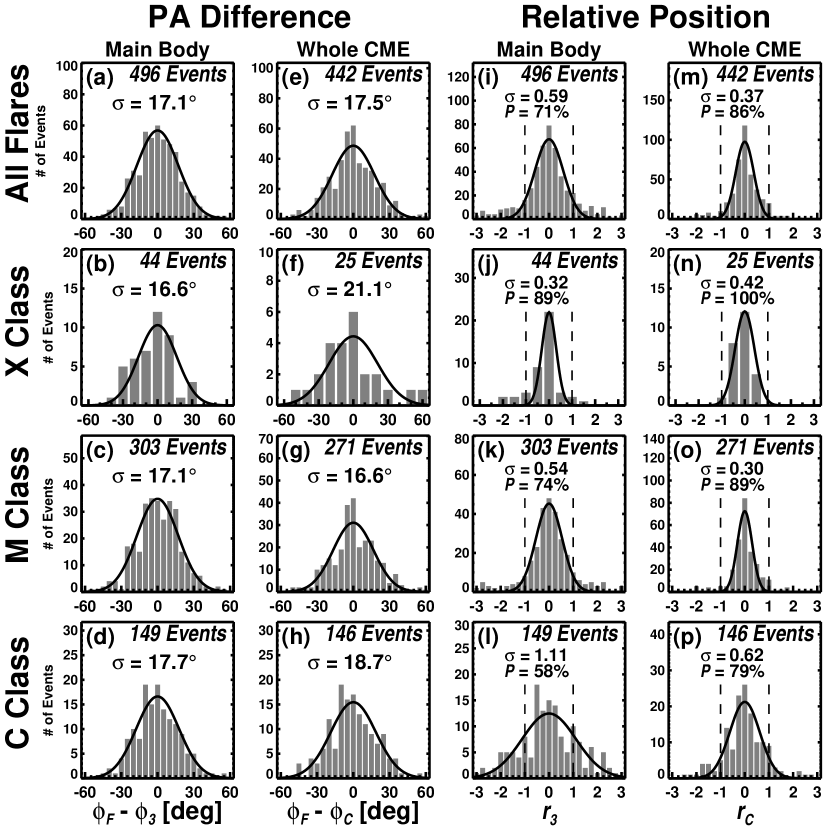
Figure 2.— Distributions of flare positions with respect to the CPA of the CME. The first and second columns show the PA difference in degree for the main CME body and for the whole CME, respectively. The standard deviation ($\sigma$) obtained by Gaussian fit is shown in each plot. The third and forth columns show the distributions of PA differences normalized by the half CME span. The vertical dashed lines mark the two side edges of the CMEs. $P$ is the percentage of the flares lying inside of the CME span. The second, third, and forth rows correspond to the events with X-class, M-class, and C-class flares, respectively.

Figure 1 illustrates how we measured the PAs of the main CME body and the whole CME. Top panels are LASCO C2 images for three CMEs with the corresponding running difference images (previous images are subtracted to enhance the faint structure of the CMEs) in the bottom panels. The side edges of the main CME body (the whole CME) are denoted by $\phi_{1}$ and $\phi_{2}$ ($\phi_{A}$ and $\phi_{B}$). The CME on 1997 November 14 (Figs. 1a and 1b) did not have an envelope, thus the $\phi_{1}$ ($\phi_{2}$) and $\phi_{A}$ ($\phi_{B}$) are identical. On the other hand, the CME on 2000 June 25 had a faint envelope to the north of the main CME body (Figs. 1c and 1d). Since it is hard to see it in print, we traced out the edge of the envelope by a dotted curve on Fig. 1d. The northern edge of the envelope denoted by $\phi_{B}$ is used for the edge of the whole CME. The black-and-white radial features (denoted by $S$) at both sides of the CME are a signature of streamer shift caused by the expansion of the CME. We should note that we did not use them for the determination of the edges of the whole CME. Since we can not see an envelope to the south of the CME, the southern edges of the main CME body and whole CME ($\phi_{1}$ and $\phi_{A}$) are almost identical. The CME on 2005 July 14 appeared in the C2 FOV at 10:54 UT (Figs. 1e and 1f). The CME had a clear three-part structure with a faint envelope. The envelope covered the occulting disk at 11:54 UT, thus the CME is listed as a halo (Howard et al., 1982) in the CME catalog. In this case $\phi_{A}$ and $\phi_{B}$ cannot be defined.

The location of a CME is represented by the central position angle (CPA), which is defined as the mid-angle of the two side edges of the CME in the sky plane. We define the CPA of the main CME body as $\phi_{3}=(\phi_{1}+\phi_{2})/2$ and that of the whole CME as $\phi_{C}=(\phi_{A}+\phi_{B})/2$. The PAs of flares ($\phi_{F}$) are computed from their location in heliographic coordinates listed in NOAA SGD. The angular span of the main CME body ($\omega_{3}$) and the whole CME ($\omega_{C}$) is defined as the difference between the two side edges [$\omega_{3}=\phi_{2}-\phi_{1}$; $\omega_{C}=\phi_{B}-\phi_{A}$].

3. Results

3.1. PA Difference

The distributions of differences between flare PAs and CME CPAs for the main CME body and for the whole CME are shown in Figures 2a and 2e, respectively. Fifty four halo CMEs are not used in Figure 2e since their $\phi_{C}$ cannot be defined. Both the distributions are very similar and are well represented by Gaussians. The standard deviation is 17.1^∘ for the difference between the flares and main CME bodies and 17.5^∘ for the difference between the flares and whole CMEs. The average (median) angular span is 52.2^∘ (43.8^∘) for the main body of CMEs and 89.5^∘ (75.0^∘) for the whole CMEs. Thus the PA differences between flares and CMEs are smaller than the angular span of the CMEs. One might think that the flare site is inherently close to the center of the CME and the non-radial motion below the C2 occulting disk produces the PA differences. In order to explain a difference of 17^∘, a CME needs to erupt 30^∘ away from the radial direction.

We separated the events into three groups according to their flare intensity and made the same plots for each group. The second, third, and forth rows in Figure 2 correspond to the events with X-class, M-class, and C-class flares, respectively. The standard deviation is shown in each plot, which ranges from 16.6^∘-17.7^∘ for the main CME body and 16.6^∘-21.1^∘ for the whole CME. The distributions of PA differences in the three groups are almost identical, suggesting that the events with weak flares (below C3 level) have a similar distribution.

3.2. Relative PA Difference

In order to investigate the flare position with respect to the main CME body (frontal structure), we normalize the PA differences by the half angular span. We define relative flare location $r_{3}=(\phi_{F}-\phi_{3})/0.5\omega_{3}$. The $r_{3}=\pm 1$ indicates the flare is located at either leg of the CME frontal structure. The $r_{3}=0$ indicates that the flare is located at the center of the CME span. The distribution of $r_{3}$ is shown in Figure 2i. It is clear that most of the flares are located under the span of the main CME body. Out of the 496 flares, 350 (or 71%) resided under the span of the main CME body. Figure 2m is the same as the Figure 2i, but for flare locations with respect to the edges of the whole CMEs [$r_{C}=(\phi_{F}-\phi_{C})/0.5\omega_{C}$]. Again, we exclude 54 full halos ($\omega_{C}=360^{\circ}$). Out of the 442 flares, 379 (or 86%) resided under the angular span of the whole CMEs. Both the distributions are well represented by Gaussians with standard deviations of 0.59 for the main CME body and 0.37 for the whole CME. In both the cases, the peak of the Gaussian is around zero, meaning that the flares frequently occur under the center of the CME span, not near one leg (outer edge) of the CMEs.

As we did for the PA difference distributions, we separated the events into three groups according to their flare intensity. The second, third, and forth rows in Figure 2 correspond to events with X-class, M-class, and C-class flares, respectively. $\sigma$ is the standard deviation and $P$ is the percentage of the flares occurring under the CME span. We found that all distributions have a peak around zero, while the width of the distributions is different for different flare levels. The flare-CME events with X-class flares (hereafter X-class events) have a narrower distribution suggesting that many X-class flares lie under the center of the CME span. On the other hand, the C-class events have a broader distribution and a significant number of events occurred outside of the CME span.

We do not see a significant distinction in the PA difference distributions among the three flare levels, but we do see a difference in the relative position distributions. Since the relative position is defined by the PA difference normalized by the CME half span, the distinction shown in Figure 2 results from the difference in CME span. The average angular span of the main CME body (the whole CME) is 87^∘ (224^∘), 54^∘ (124^∘), and 38^∘ (75^∘) for X-, M-, and C-class events, respectively. As reported by the previous studies (e.g., Yashiro et al., 2005), by means of statistics, CMEs associated with stronger flares have larger angular span.

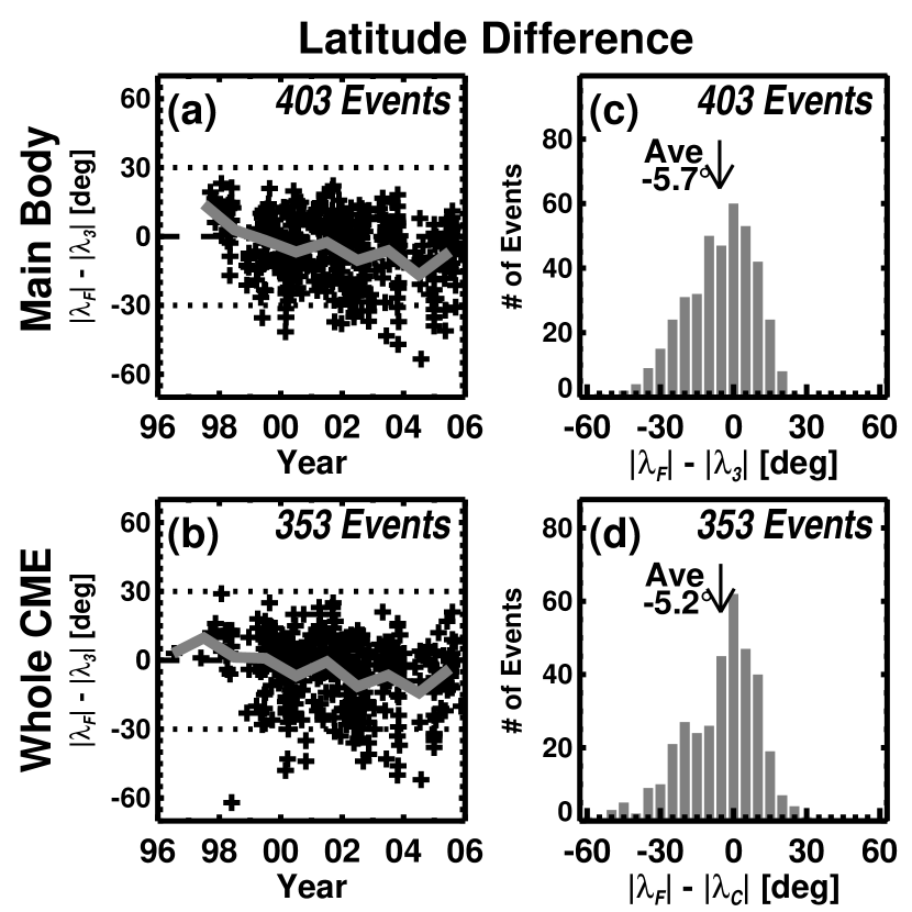
Figure 3.— Solar cycle variation (left) and distribution (right) of the latitude difference between flares and CMEs. $\lambda_{F}$, $\lambda_{3}$, and $\lambda_{C}$ are latitudes of the flares, main CME body, and whole CME, respectively. The flare-CME pairs occuring in different hemispheres (e.g. a flare in the northern hemisphere and a CME in the southern) were excluded.

3.3. Latitude Difference

Even though the flare PAs tend to be close to those of CMEs, we need to point out some systematic offsets between flares and CMEs stemming from the varying influence of the global solar magnetic field as a function of the solar cycle. Gopalswamy et al. (2003a) examined the relationship between prominence eruptions (PEs) and CMEs and found that, during solar minimum, the CPA of CMEs tend to be closer to the equator compared to those of PEs, while no such effect was seen during solar maximum. A similar relation is expected between flares and CMEs. In order to examine whether flare positions are equatorward or polarward with respect to the CMEs, we have shown their latitudinal differences in Figures 3. The CME latitudes ($\lambda_{3}$ and $\lambda_{C}$) were calculated from CPAs of the main CME body ($\phi_{3}$) and whole CME ($\phi_{C}$), respectively. The flare-CME pairs occurring in different hemispheres were excluded.

The gray lines in Figs 3a and 3b show annual average of the latitude difference. In spite of the small data set during solar minimum, we see a positive offset in 1997, meaning that CMEs occurred in lower latitudes as compared to flares. This is consistent with the result of Gopalswamy et al. On the other hand, during solar maximum, we see a negative offset, indicating that flares occurred in lower latitudes as compared to CMEs. This is different from Gopalswamy et al. who reported that no systematic offset exists between PE and CME latitudes. The difference may result from the exclusion of high-latitude flares from our analysis. Since we did not include small flares (below C3 level), the high-latitude flares (e.g. X-ray arcade formations associated with the eruption of polar crown filaments) were excluded. Therefore the sampled flares mainly occurred in active regions, i.e. in low latitudes. We should note that high-latitude CMEs are not associated with active-region flares, but appear frequently during solar maximum (Gopalswamy et al., 2003b). During the declining phase of solar cycle 23, CMEs have gradually started clustering around the equator, while active regions have remained around the equator. This is why we still see the negative offset in 2004 and 2005. The positive offset between flare and CME latitude is likely to resume with the start of solar cycle 24.

One would think that the existence of the latitude offset is inconsistent with the result that flares frequently occur under the center of the CME span. In order to check this, we have shown the distributions of latitude differences in figures 3c and 3d. Because of the exclusion of the flare-CME events from different hemispheres, the distributions became narrower since the excluded events have relatively larger PA differences. We can see that both the distributions are asymmetric with a broad tail on the left. However, the most frerqent bin stays as 0^∘ and the average (median) difference is -5.7^∘ (-3.9^∘) for the main CME body and -5.2^∘ (-2.0^∘) for the whole CME. We conclude that there are systematic offsets between flares and CMEs, but such an offset is only a small fraction ($\sim 10\%$) of the CME span.

4. Summary & Discussion

We investigated the spatial relationship between solar flares and CMEs for 496 pairs occurring from 1996 to 2005. It is found that the distribution of the difference between flare PA and CME CPA can be represented by Gaussian centered at zero with a standard deviation of $\sim 17^{\circ}$, and the distribution does not change with the flare level. We examined the flare positions with respect to the CME span and found that the most probable flare site is the center of the CME span for all flare levels, but the width of the distributions is different for different flare levels. For C-class events, the flare positions widely scattered with respect to the CME span, while for X-class events, most of the flares lie under the center of the CME span. The result is suitable for flare-CME models typified by the CSHKP reconnection model.

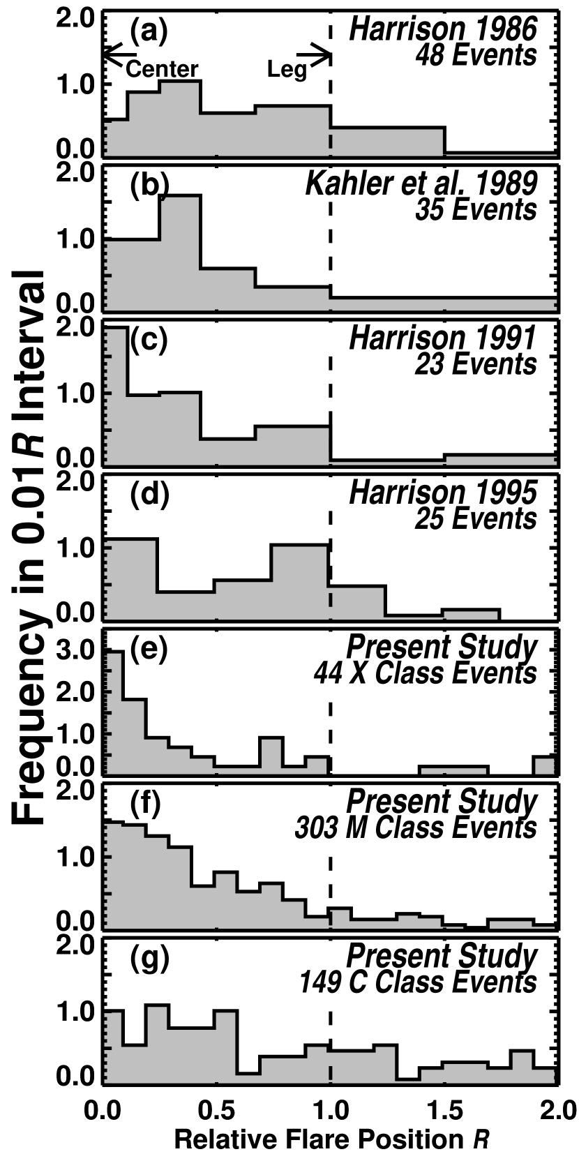
Figure 4.— Flare position ($R$) with respect to the CME span. $R=0$ for a flare centered under the CME, $R=1$ for a flare at one leg of the CME, and $R>1$ for a flare lying outside of the CME span.

Table 1Summary of studies on the spatial relationship between flares and CMEs

	# of Events	Satellite	Data Period	Remarks
Harrison 1986 (H86)	48	Solwind and SMM	$1979-82$	$\cdots$
Kahler et al. 1989 (K89)	35	Solwind	$1979-82$	$I_{P}$ $\geq$ M1; CMD $\geq 45^{\circ}$; WD $\geq 40^{\circ}$
Harrison 1991 (H91)	23	SMM	$1984-87$	$\cdots$
Harrison 1995 (H95)	25	SMM	$1986-87$	CMD $\geq 40^{\circ}$
Present Study	496	SOHO	$1996-05$	$I_{P}\geq$ C3; CMD $\geq 45^{\circ}$

4.1. Comparison with Previous Studies

Let us compare our results with four previous studies, Harrison (1986, hereafter H86), Kahler et al. (1989, hereafter K89), Harrison (1991, hereafter H91), and Harrison (1995, hereafter H95). All previous studies examined flare positions with respect to the CME span using data obtained by Solwind or SMM. Since the observational capability of the pre-SOHO coronagraphs is thought to be lower, it is possible that they did not detect the faint envelope around the three-part CME structure. Therefore, for the proper comparison, we used $r_{3}$, the flare positions with respect to the main CME body.

H86 employed the parameter $\alpha=(\phi_{2}-\phi_{F})/(\phi_{F}-\phi_{1})$ (In Figure 4 of H86, $\phi_{2}$, $\phi_{F}$, and $\phi_{1}$ correspond to letters $A$, $B$, and $C$). He found a significant peak at $\alpha=0-0.19$, meaning that flares often occur at the one leg of the CMEs. However, K89 pointed out that the bin size in equal $\alpha$ is biased; the smallest bin ($\alpha=0-0.19$) is about 3 times more probable than the largest bin ($\alpha=0.8-1.0$) for the random distribution of flare positions. They employed the parameter $R=|\phi_{F}-\phi_{3}|/0.5\omega_{3}$, which is the absolute of $r_{3}$. The relation between parameters $\alpha$ and $R$ is $R=(1-\alpha)/(1+\alpha)$.

In order to compare the previous studies properly, we converted the distributions in equal $\alpha$ into those in equal $R$. For each $\alpha$ bin, the frequency ($f$) in 0.01 $R$ intervals in percentage is computed by dividing the number of events ($n$) by both the total number of events ($N$) and the interval of $R$ ($dR$), i.e. $f=n/N/dR$. For example, H86 examined 48 flare-CME events and found that 3 of them are in the bin of $\alpha=0.8-1.0$, which corresponds to $R=0-0.11$ ($N=48$, $n=3$, and $dR=0.12$). Then we obtained the frequency for $R=0-0.11$ bin to be 0.52 (=3/48/0.12). We carried out the same conversion for other bins. However, treatment of the $\alpha=0-0.19$ bin is not easy. Harrison used 30 Solwind events compiled by Sheeley et al. (1984) and 18 SMM events compiled by Sawyer. We examined the Sheeley et al.’s list and found 7 events lying outside the CME span. Such flares should have negative $\alpha$, but there is no corresponding bin in Fig. 5 of H86. Thus we supposed that the 7 events were included in $\alpha=0-0.19$ bin, and determined their $R$ using the Sheeley et al’s list. Unfortunately we could not locate Sawyer’s 18 events. Thus we assumed that the same fraction of the events in the bin inherently lied outside of the CME span. The result of this analysis is shown in Figure 4a. By the conversion of equal $\alpha$ to equal $R$ distribution and the special treatment of $\alpha=0-0.19$ bin, the peak at the $\alpha=0-0.19$ bin in Fig. 5 of H86 disappeared. For K89, we obtained the $R$ distribution from their Table 3. They reported 7 out of the 35 flares occurring outside the CME span. However we could not find out how far apart the flares were located from the nearest CME leg. Thus we assumed that the 7 events resided in $R=1.01-2.00$. The $R$ distribution of K89 is shown in Figure 4b. H91 has a histogram of the $\alpha$ distribution and their conversion to the $R$ distribution was straightforward (Fig. 4c). H95 does not have a histogram of spatial distribution, but has the scatter plots of $R$ vs. flare intensity and $R$ vs. flare duration. We read the $R$ value from the plots and made a histogram of the $R$ distribution (Fig. 4d). For the present study, we plotted the $R$ distribution for the X-class, M-class, and C-class events in Figure 4e, 4f, and 4g, respectively.

As we showed in Section 3.2, the $R$ distribution varies according to the scale of the flare-CME events. Therefore, in the comparison with previous studies, we should pay attention to their data source and selection criteria, which are summarized in Table 1. The second and third columns show that the number of events and satellites used in each study. The forth column shows the study period. H86 and K89 used data during solar maximum, while H91 and H95 used data during solar minimum. The present study covers the almost whole of the solar cycle 23, but many events were obtained during solar maximum. The last column is for event selection criteria in each study. K89 and the present study used only strong flares ($\geq$ M1 and $\geq$ C3, respectively), but other studies by Harrison did not eliminate weak flares. K89, H95, and the present study used limb events only, which reduces the projection effects.

Except for H95 (Fig. 4d), the three previous studies show a trend that the flare occurred near the center of CMEs rather than at the edges. The majority of the events in H95 were C-class flares, thus we should compare the result of H95 with our C-class events (Fig. 4g). The C-class events in our data show a trend that flare occurred near the CME center, but the trend is very weak. Therefore it is not surprising that the examination of the 25 events can not see such weak trend. On the other hand, H91 shows a strong peak at the center of the CME even though the data were obtained during solar minimum (1984-87). We could not find a statement of exclusion of disk events, thus the projection effects might produce the peak (Apparent CME span becomes larger than inherent span if the distance from the limb is farther). Except for the lack of flares under the center of the CME span ($R<0.25$), the $R$ distribution of K89 (Fig. 4b) is similar to that of our M-class events (Fig. 4f), which can be explained by their selection criterion about flare intensity ($\geq$ M1 level). By the same token, because 30% and 57% of the H86 events were X-class and M-class flares, respectively, Fig. 4a should be the similar to Fig. 4e or Fig. 4f. However the distribution is similar to that of C-class events (Fig. 4g). Additionally H86 also lacks flares under the center of the CME span ($R<0.25$). The average CME span of H86 events (64^∘) is larger than that of our M-class events (56^∘), suggesting that the different capability between SOHO LASCO and previous coronagraphs does not explain the H86 lack of flares under the center of the CME span. Except for this discrepancy, all the flare position distributions reported in the previous studies are consistent with our results. The long-term LASCO observation enabled us obtain a large number of flare-CME pairs from small to large events for the first time that revealed the detailed spatial relation between flares and CMEs.

4.2. Flare-CME Geometry

The flare-CME asymmetry found by H86 has been the basis of the claim that flare-CME observations are inconsistent with the schematic picture of the CSHKP type flare-CME models. In this paper we show that most of the X-class flares are located at the center of the CME span while a significant number of C-class flares reside near the edge or even outside of the CME span. The CSHKP type flare-CME models are well suited for strong events, but may not be applicable for the many weak events. The other extreme is the non-eruptive (or compact) flares which do not involve any mass motion, and hence their geometry may not be appropriate for CSHKP models.

The flare-CME geometry is possibly different between weak (narrow) and strong (wide) events. This is related to the issue whether narrow CMEs are physically distinct from general CMEs (Kahler et al., 1989, 2001). Reames (2002) presented two types of flare-CME geometry which are responsible for two types of solar energetic particle (SEP) events, i.e. impulsive and gradual events. The gradual SEP events are associated with large CMEs, which fit CSHKP type models, while the impulsive SEPs are associated with narrow CMEs that fit the X-ray jet model (Shimojo & Shibata, 2000). Bemporad et al. (2005) reported that blob-like narrow CMEs in a streamer (called ”streamer puffs”) differ from general CMEs (see also Moore & Sterling, 2007). The streamer puffs are associated with weak flares (below C4 level) and their schematic picture clearly explains the flare-CME asymmetry.

Even X-class events, some of them showed the clear flare-CME asymmetry. A good example is the event on 2002 May 20. The X2.1 flare at 15:21 UT located at one edge of the CME at 15:50 UT. Another example is the event on 2003 November 3 (The X2.7 flare at 01:09 UT and the CME at 01:59 UT). In both cases EIT dimmings were clearly observed only on the CME side of the flares. It is important to investigate the flare-dimming asymmetry for understanding the origin of such flare-CME asymmetry.

We examined the flare positions with respect to CME spans using LASCO data and found that most frequent flare site is the center of the CME span. However, since we examined the spatial relationship using limb events, our finding can apply only in the latitudinal direction. The flare-CME geometry in the longitudinal direction has never been examined. The Solar TErrestrial RElations Observatory (STEREO) mission started to observe CMEs in stereoscopic view. Three-dimensional structure of the CMEs and their relation to the associated flares should be tested again using STEREO data.

References

- Bemporad et al. (2005) Bemporad, A., Sterling, A. C., Moore, R. L., & Poletto, G. 2005, ApJ, 635, L189
- Brueckner et al. (1995) Brueckner, G. E., et al. 1995, Sol. Phys., 162, 357
- Ciaravella et al. (2005) Ciaravella, A., Raymond, J. C., & Kahler, S. W. 2005, ApJ, 621, 1121
- Gilbert et al. (2001) Gilbert, H R., Serex, E. C., Holzer, T. E., MacQueen, R. M., & McIntosh, P. S. 2001, ApJ, 550, 1093
- Gopalswamy et al. (2000) Gopalswamy, N., Hanaoka, Y., & Hudson, H. S. 2000, Adv. Sp. Res., 25(9), 1851
- Gopalswamy et al. (2003a) Gopalswamy, N., Shimojo, M., Lu, W., Yashiro, S., Shibasaki, K., & Howard, R. A. 2003a, ApJ, 586, 562
- Gopalswamy et al. (2003b) Gopalswamy, N., Lara, A., Yashiro, S., & Howard, R. A. 2003b, ApJ, 598, L63
- Harrison (1986) Harrison, R. A. 1986, A&A, 162, 283
- Harrison (1991) Harrison, R. A. 1991, Adv. Space Res., 11, 25
- Harrison (1995) Harrison, R. A. 1995, å, 304, 585
- Harrison (2006) Harrison, R. A. 2006, in Solar Eruptions and Energetic Particles, AGU Monograph 165, 73
- Howard et al. (1982) Howard, R. A., Michels, D. J., Sheeley, N. R., & Koomen, M. J. 1982, ApJ, 263, L101
- Illing & Hundhausen (1985) Illing, R. M. E. & Hundhausen, A. J. 1985, J. Geophys. Res., 90, 275
- Kahler et al. (1989) Kahler, S. W., Sheeley, N. R., & Ligget, M. 1989, ApJ, 344, 1026
- Kahler et al. (2001) Kahler, S. W., Reames, D. V., & Sheeley, N. R. 2001, ApJ, 562, 558
- Moore & Sterling (2007) Moore, R. L. & Sterling, A. C. 2007, ApJ, 661, 543
- Reames (2002) Reames, D. V. 2002, ApJ, 571, L63
- Sheeley et al. (2000) Sheeley, N. R., Hakala, W. N., & Wang, Y.-M. 2000, J. Geophys. Res., 105, 5081
- Shimojo & Shibata (2000) Shimojo, M. & Shibata, K. 2000, ApJ, 542, 1100
- St. Cyr (2005) St. Cyr, O. C. 2005, Eos Trans. AGU, 86(30), 281
- Vourlidas et al. (2003) Vourlidas, A., Wu, S. T., Wang, A. H., Subramanian, P., & Howard, R. A. 2003, ApJ, 598, 1392
- Webb (1988) Webb, D. F. 1988, J. Geophys. Res., 93, 1749
- Webb & Hundhausen (1987) Webb, D. F. & Hundhausen, A. J. 1987, Sol. Phys., 108, 383
- Yashiro et al. (2004) Yashiro, S., Gopalswamy, N., Michalek, G., St. Cyr, O. C., Plunkett, S. P., Rich, N. B., & Howard, R. A. 2004, J. Geophys. Res., 109, 7105
- Yashiro et al. (2005) Yashiro, S., Gopalswamy, N., Akiyama, S., Michalek, G., & Howard, R. A. 2005, J. Geophys. Res., 110, A12S05
- Zhang et al. (2004) Zhang, J, Dere, K. P., Howard, R. A., & Vourlidas, A. 2004, ApJ, 604, 420