Effect of electron-electron interaction on the Fermi surface topology of doped graphene.

Abstract

The electron-electron interactions effects on the shape of the Fermi surface of doped graphene are investigated. The actual discrete nature of the lattice is fully taken into account. A $\pi$-band tight-binding model, with nearest-neighbor hopping integrals, is considered. We calculate the self-energy corrections at zero temperature. Long and short range Coulomb interactions are included. The exchange self-energy corrections for graphene preserve the trigonal warping of the Fermi surface topology, although rounding the triangular shape. The band velocity is renormalized to higher value. Corrections induced by a local Coulomb interaction, calculated by second order perturbation theory, do deform anisotropically the Fermi surface shape. Results are compared to experimental observations and to other theoretical results.

I Introduction

Since its discovery Novoselov and Geim (2004); Novoselov et al. (2005); Zhang et al. (2005) graphene, a two-dimensional (2D) single crystal thermodynamically stable formed by a single-layer of carbon atoms ordered in a honeycomb lattice, has been thoroughly investigated. It forms the basic block of carbon nanotubes, fullerenes, graphite, and graphite intercalation compounds. The 2D electronic properties are well described by a $\pi$-band tight-binding (TB) model Wallace (1947). The valence and conduction $\pi$-bands touch only at the six corners, K, of the 2D Brillouin zone (BZ); the degeneracy point of the valence and conduction bands is often termed Dirac point. At half-filling, undoped graphene, the Fermi level $E_{F}$ lies at the Dirac point. The low-energy physics of a perfect graphene sheet is described by the relativistic Dirac equation. The dispersion relation turns up to be isotropic and linear near $E_{F}$. The low-energy excitations of the system are Dirac fermions with zero effective mass and a vanishing density of states at the K points. Because of these peculiarities, graphene is considered a model system to investigate basic questions of quantum mechanics. Due to its transport properties graphene is a promising material for nanoelectronic applicationsNeto et al. (2007).

Improvements in experimental resolution have led to high precision measurements of the Fermi surface (FS), and also to the extraction of the many-body effects from the spectral function, as reported by angle resolved photoemission spectroscopy (ARPES) experiments Damascelli et al. (2003) in different materials. The recent isolation of an atomic layer of graphite, graphene, has renewed the interest in the physics of the three-dimensional (3D) graphite and new aspects of the electronic properties of 3D graphite have been observed with improved experimental techniquesKopelevich and Esquinazi (2007).

In a high resolution ARPES study of disordered graphite samples, coexistence of sharp quasiparticle dispersions and disordered features was found Zhou et al. (2005), and was explained in terms of Van Hove singularities (VHS) in the angular density of states. Later on, by using ARPES, the linear and isotropic dispersion of the bands, near the three-dimensional BZ corners (H points) of graphite, has been directly observed coexisting with parabolic dispersion bands Zhou et al. (2006). The constant energy maps taken near the H point present circular shape from $E_{F}$ to $-0.6$eV. This circular shape combined with the linear dispersion found near the BZ corners H suggests that the dispersion shows a cone-like behavior near each point H, similar to that expected for graphene. The constant energy maps start to deviate from the circular shape at $-0.9$eV, and at $-1.2$eV a rounded triangular shape is observed. A linear energy dependence of the quasiparticle life-time has been as well measured by ultrahigh resolution ARPES on high quality crystals of graphite Sugawara et al. (2007). The low-energy excitations seem to be dominated by phonons, while those for higher energies are characterized by the electron-hole pair creationSugawara et al. (2007). The quasiparticle life-time had been studied as well by ultrafast time resolved photoemission spectroscopy (TRPES) Xu et al. (1996) and a linear $\omega$ dependence was reported. Anisotropy of quasiparticle life-times has been reported by TRPES in highly oriented pyrolytic graphite (HOPG) as well as an anomaly in the energy dependence between $1.1$ and $1.5$eV, in the vicinity of a saddle point in the graphite band structure Moos et al. (2001).

A linear energy dependence of the quasiparticle lifetime had been theoretically predicted for graphiteGonzález et al. (1996a) neglecting the interlayer hopping. Even including an interlayer hoping of $0.25$eV, an anomalous quasiparticle life-time was obtained in graphiteSpataru et al. (2001) within the $GW$ approximation, with a linear energy dependence along the $\bf{K\Gamma}$ direction for energies well above the interlayer hoping. A discussion about the interlayer coupling strength in graphite can be found in Refs.López-Sancho et al. (2007); Kopelevich and Esquinazi (2007), along side with an overview of recent experiments in both graphene and graphite samples.

In a combined ARPES and theoretical ab-initio quasiparticle study of the $\pi$-band structure and the Fermi surface in graphite single crystals, it is found that electron-electron correlation plays an important role in semi-metallic graphite and should be taken into account for the interpretation of experimental results Grüneis et al. (2008). The electronic correlations renormalize the electronic dispersion increasing the Fermi velocity. The equi-energy contours of the photoemission intensity show trigonal warping (higher by a factor of about 1.5 if compared to graphene) around the KH direction of the graphite 3D BZ, in both Local Density Approximation (LDA) and TB-$GW$ calculations, from $-0.1$eV. Correlation effects are found to be stronger as the energy increases and differences between LDA and $GW$ results are more noticeable at $-0.4$eV than at $-0.1$eV Grüneis et al. (2008).

The recently available 2D graphene samples have been intensively investigated. From the experimental point of view graphene presents advantages with respect to other 2D systems. Graphene can be controlled externally and exposed to vacuum therefore can be directly probed by different techniques Novoselov and Geim (2004); Novoselov et al. (2005); Zhang et al. (2005). Electron-electron interactions in graphene are expected to play an important role due to its low dimensionality and many-body effects have received great attention. The quasiparticle dynamics in graphene samples has been addressed by high-resolution ARPES Bostwick et al. (2007). It was found that the conical bands are distorted due to many-body interactions, which renormalize the band velocity and the Dirac crossing energy $E_{D}$. Electron-hole pair generation effects are important near the Fermi energy and electron-phonon coupling contribution to the self-energy is also important in the Fermi level region: an electron-phonon coupling constant of $\lambda\approx 0.3$ is deduced with the standard formalismBostwick et al. (2007). Around $E_{D}$, electron-plasmon coupling is invoqued to explain the peak in the imaginary part of the self-energy ${\rm Im}\Sigma$, found just below $E_{D}$, whose width (and intensity) scales with $E_{D}$. Although the three scattering mechanisms contribute to strongly renormalize the bands, in Ref. Bostwick et al. (2007) it is claimed that the quasiparticle picture is valid over a spectacularly wide energy range in graphene. More recently, the doping dependence of graphene electronic structure has been investigated by ARPES in graphene samples at different dopings McChesney et al. (2007). Upon doping with electrons, the Fermi surface grows in size and deviates from the circular shape showing the trigonal warping, finally evolving into a concave triangular shape. An electron-phonon coupling to in-plane optical vibrations is proposed to explain the experimental results. The electron-phonon coupling constant, extracted from the data, presents a strong dependence on $\vec{\bf k}$, with maximal value along the KM direction. The presence of a Van Hove singularity in the KMK direction, confirmed upon doping, could be a possible explanation of the enhancement of the electron-phonon couplingMcChesney et al. (2007).

The layered nature of graphite/graphene as well as the presence of the VHS in the density of states near the $E_{F}$, which would enhance many-body effects, make contact with the physics of cuprates superconductors. The similarities between graphene and the cuprates have been already noticed Bena and Kivelson (2005) and the important role of many-body effects in the basic physics of graphene has been investigated earlier González et al. (1993).

ARPES investigation of graphene samples epitaxially grown on SiC substrate, have reported the observation of an energy gap of $\approx 0.26eV$ at the K point Zhou et al. (2007). It is proposed that the opening of the gap is induced by the interaction with the substrate on which graphene is grown, that breaks the A and B sublattice symmetry Zhou et al. (2007).

From the theoretical point of view, graphene offers many possibilities and the electron-electron interaction induced effects have been widely analyzed. The self-energy have been object of special interest, since it gives relevant information from fundamental properties. Furthermore, theoretical results can be compared to recent ARPES reported self-energies. Many approximations have been followed to investigate the self-energy in graphene. The inelastic quasiparticle lifetimes have been obtained within the $G_{0}W$ approximation Hwang et al. (2007) with a full dynamically screened Coulomb interaction. The scattering rates calculated for different carrier concentrations are in good agreement with ARPES data from Bostwick $et\,\,al.$ Bostwick et al. (2007) without including phonon effects, contrary to the experimental interpretation of the data Bostwick et al. (2007). The nature of the undoped and doped graphene has been as well discussed theoretically in terms of the behavior of the imaginary part of the self-energy Sarma et al. (2007a): a Fermi liquid behavior is found for doped graphene while the zero doping case exhibits a quasiparticle lifetime linear and a zero renormalization factor indicating that, close to the Dirac point, undoped graphene behaves as marginal Fermi liquid, in agreement with previous theoretical workGonzález et al. (1996a); González et al. (1999).

By evaluating exchange and random-phase-approximation (RPA) correlation energies, an enhancement of the quasiparticle velocities near the Dirac point is found in lightly doped graphene taking into account the eigenstate chirality Barlas et al. (2007). The role of electron-electron interactions in the ARPES spectra of a n-doped graphene sheet has been theoretically investigated Polini et al. (2007) by evaluating the self-energy within the RPA and turned out to be important when interpreting experimental data. Recently Mishchenko (2007); Sarma et al. (2007b) the validity of the RPA in the calculation of graphene self-energy has been discussed. The approximation is shown to be valid and controlled for doped graphene where the Fermi level is shifted up or down from the Dirac point. The RPA fails for undoped graphene, where $E_{F}$ lies at $E_{D}$. In most of the self-energy studies graphene is described by the massless Dirac equation in the continuum limit.

In this work, we calculate the corrections induced by the electron-electron interaction on the electronic band structure. We focus on the corrections to the Fermi surface shape of doped graphene. The Fermi surface is one of the key features needed to understand the physical properties of a material and its shape provides important information. Due to the 2D character of graphene, electronic interaction should be important. We consider the $\pi$-band tight-binding model taking into account the discrete nature of the honeycomb lattice in order to investigate doped graphene and possible correlation effects in the trigonal warped topology of the Fermi surface. We calculate first the exchange self-energy considering long- and short-range Coulomb interactions. Besides the renormalization of the band velocities, a deformation of the trigonal warped Fermi surface is found at this level. The second-order self-energy induced by an onsite Coulomb interaction is as well calculated. The corrections to the Fermi surface shape are found to be anisotropic.

The paper is organized as follows. In section II the model is presented and we explain the self-energy calculation method. Section III presents the results of the calculation and Section IV contains a discussion of the results compared to experimental data and to other theoretical results and the main conclusions of the work.

II The method

II.1 The model for the graphene layer

Graphene is an atomic layer of carbon atoms arranged in a honeycomb lattice with two atoms per unit cell, as shown in Fig.1. The distance between nearest neighbor atoms is $a=1.42{\rm\AA}$, and the primitive lattice vectors are $\vec{\bf a}_{1}$ and $\vec{\bf a}_{2}$. The Brillouin zone is an hexagon, as depicted in Fig.1. We adopt the $\pi$-band tight-binding model with only nearest-neighbor hoppingWallace (1947), since it captures the main physics of the system as probed by more realistic models and by experimental results.

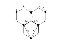
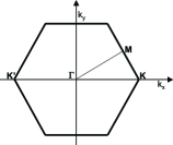
Figure 1: (a) Schematic representation of the structure of the honeycomb lattice, open and solid points represent the two inequivalent atoms. The basic vectors $\vec{\bf a}_{1}$ and $\vec{\bf a}_{2}$ of the lattice are shown. The three $\vec{\tau_{i}}$ connect nearest neighbor atoms. (b) First Brillouin zone of the honeycomb lattice.

The kinetic term of the Hamiltonian, considering only nearest-neighbor hopping, will be (we choose $\hbar=1$ throughout this paper)

$${\cal H}_{kin}=-t\sum_{\langle ij\rangle,\sigma}{\hat{a}}^{\dagger}_{i,\sigma}{\hat{b}}_{j,\sigma}+h.c.$$ (1)

where $t=2.82$eV is the nearest-neighbor hopping parameter, and the site energy of the $2p_{z}$ atomic orbital is taken as zero. The operator ${\hat{a}}^{\dagger}_{i,\sigma}$ (${\hat{a}}_{i,\sigma}$) is the creation (annihilation) operator of an electron at site ${\vec{\bf R}}_{i}$ on sublattice A with spin $\sigma$ ($\sigma=\uparrow,\downarrow$) (an equivalent definition corresponds to sublattice B). By Fourier transformation to the momentum space we have

$${\cal H}_{kin}(\vec{\bf k})=t\left(\begin{array}[]{cc}0&g(\vec{\bf k})\\ g^{*}(\vec{\bf k})&0\\ \end{array}\right)$$ (2)

The function $g(\vec{\bf k})$

$$g(\vec{\bf k})=-\left(e^{-ik_{y}a}+2e^{ik_{y}a/2}\cos\left(\dfrac{\sqrt{3}}{2}k_{x}a\right)\right).$$ (3)

is the structure factor of the honeycomb lattice. Diagonalizing Eq.(2) the energy dispersion relation $\epsilon^{0}_{\lambda}(\vec{\bf k})=\lambda t|g(\vec{\bf k})|$ is obtained

$$\epsilon^{0}_{\lambda}\!(\vec{\bf k})\!\!=\!\!\lambda t\sqrt{\!1\!\!+\!\!4\cos\!\!\left(\!\dfrac{3}{2}ak_{y}\!\right)\!\!\cos\!\!\left(\!\dfrac{\sqrt{3}}{2}ak_{x}\!\right)\!\!+\!\!4\cos^{2}\!\!\left(\!\dfrac{\sqrt{3}}{2}ak_{x}\!\right)}$$ (4)

where $\lambda=-(+)$ for the valence (conduction) band. The two bands are degenerated at the six corners of the BZ, $\bf{K}$ points. The corresponding Bloch wave functions are

$$\Psi_{\vec{\bf k};\lambda}(\vec{\bf r})=\frac{1}{\sqrt{2}}\left({\cal K}_{1\vec{\bf k}}(\vec{\bf r})+\lambda\frac{g^{*}(\vec{\bf k})}{|g(\vec{\bf k})|}{\cal K}_{2\vec{\bf k}}(\vec{\bf r})\right)$$ (5)

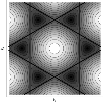
Figure 2: Constant energy contours obtained with Eq.(4). The thick black lines corresponds to the Van Hove filling.

The tight-binding functions are built from the atomic $2p_{z}$ orbitalsBlinowski et al. (1980) $\phi_{z}(\vec{\bf r})$

$${\cal K}_{i\vec{\bf k}}(\vec{\bf r})=\sqrt{\frac{A}{S}}\sum_{\vec{\boldsymbol{\rho}}_{n}}e^{\imath\vec{\bf k}\cdot(\vec{\boldsymbol{\rho}}_{n}+\vec{\boldsymbol{\tau}}_{i})}\phi_{z}(\vec{\bf r}-\vec{\boldsymbol{\rho}}_{n}-\vec{\boldsymbol{\tau}}_{i})$$ (6)

where $A$ and $S$ stand for the area of the unit cell and the crystal respectively; $\vec{\boldsymbol{\rho}}_{n}=n_{1}\vec{\bf a}_{1}+n_{2}\vec{\bf a}_{2}$ is the lattice vector, and $\vec{\boldsymbol{\tau}}_{1,2}$ define the position of the two inequivalent atoms in the unit cell. We use $\vec{\boldsymbol{\tau}}_{1}=0$ and $\vec{\boldsymbol{\tau}}_{2}=\frac{1}{3}(\vec{\bf a}_{1}+\vec{\bf a}_{2})$ (see Fig.1). At half-filling (undoped graphene) the Fermi energy lies at the common point of the two bands (we take this energy as our zero energy) and the Fermi surface is formed by six points at the six BZ corners. The constant energy contours for the dispersion relation Eq.(4) are depicted in Fig.2. These six isolated points (only two of them are inequivalent) are known as Dirac points because around them, by a long-wavelength expansion, the kinetic energy term of the Hamiltonian can be approximated by the 2D Dirac equation for massless fermions. Upon doping, by following the constant energy maps shown in Fig.2, the FS points develop into circles and, eventually, the FS adopt the rounded triangular shapes . As can be seeing in Fig.2, around each of the six BZ corners the energy lines are the same but rotated with respect each other. Therefore, in the following, we will show the results in the vicinity of one of the corners of the BZ.

The electron interaction term of the Hamiltonian ${\cal H}_{int}$ includes the Coulomb interaction $e^{2}/\epsilon_{0}|\vec{\bf r}_{ij}|$, where $|\vec{\bf r}_{ij}|$ indicate distances between sites of the honeycomb lattice and $\epsilon_{0}$ is the dielectric constant. We will study the two limiting cases, long- and short-range Coulomb repulsion. Among the short-range interactions, we consider interactions between electrons on neighbor atoms of the honeycomb lattice.

We also analyze corrections due to an on-site Coulomb repulsion $U$ between electrons with opposite spin on the same $p_{z}$ atomic orbital. Although graphene is considered a weakly correlated system, the effects of an on-site Coulomb interaction, Hubbard term, on the electronic properties of the honeycomb lattice have been investigated in different scenarios. The phase diagram of the Hubbard model in the honeycomb lattice has been studied by a variety of techniques. Different instabilities have been found, from the Mott-Hubbard transition Sorella and Tosatti (1992), charge- and spin-density wave Tchougreeff and Hoffmann (1992); López-Sancho et al. (2001), to superconductivity and magnetic phases Perfetto et al. (2002); Herbut (2006, 2007). In our calculation we consider small values of the on site repulsion, of the order of the hopping parameter for graphene.

II.2 Calculation of the self-energy

II.2.1 Long- and short-range Coulomb interaction: exchange self-energy.

Figure 3: (a) First-order self-energy diagram corresponding to the exchange contribution. (b) Second-order self-energy diagram.

We calculate first the exchange self-energy contribution, that corresponds to the one-loop diagram shown in Fig.3(a). The self-energy has the form:

$$\Sigma^{x}_{\lambda}(\vec{\bf k},i\omega_{n})\!\!=\!-\!\!\!\!\!\sum_{\lambda^{\prime}=\pm}\!\!\sum_{\vec{\bf q}}\!\!\frac{1}{\beta}\sum_{i\nu_{n}}G^{0}_{\lambda^{\prime}}(\vec{\bf k}+\vec{\bf q},i\omega_{n}+i\nu_{n})v_{\lambda\lambda^{\prime}}(\vec{\bf k},\vec{\bf k}+\vec{\bf q})$$ (7)

where $\beta=1/k_{B}T$, $\omega_{n}$ and $\nu_{n}$ are fermionic and bosonic Matsubara frequencies respectively, and $G_{\lambda}^{0}(\vec{\bf k},i\omega_{n})$ is the bare single-particle Green’s function of an electron with momentum $\vec{\bf k}$ and band-index $\lambda$. The Coulomb interaction matrix elements $v_{\lambda\lambda^{\prime}}(\vec{\bf k},\vec{\bf k}+\vec{\bf q})$ between states $|\vec{\bf k},\lambda\rangle$ and $|\vec{\bf k}+\vec{\bf q},\lambda^{\prime}\rangle$, are given by

$$v_{\lambda,\lambda^{\prime}}(\vec{\bf k},\vec{\bf k}+\vec{\bf q}) = \int d\vec{\bf r}_{1}\int d\vec{\bf r}\langle\Psi_{\vec{\bf k},\lambda}(\vec{\bf r}_{1})|\langle\Psi_{\vec{\bf k}+\vec{\bf q},\lambda^{\prime}}(\vec{\bf r}_{1}-\vec{\bf r})|\frac{e^{2}}{r}|\Psi_{\vec{\bf k},\lambda}(\vec{\bf r}_{1}-\vec{\bf r})\rangle|\Psi_{\vec{\bf k}+\vec{\bf q},\lambda^{\prime}}(\vec{\bf r}_{1})\rangle$$ (8)

$$= V(\vec{\bf q})F_{\lambda\lambda^{\prime}}(\vec{\bf k},\vec{\bf k}+\vec{\bf q})$$

where $V(\vec{\bf q})$ is the 2D Fourier transform of the Coulomb interaction

$$V^{lr}(\vec{\bf q})=\frac{2\pi e^{2}}{\epsilon_{0}|\vec{\bf q}|}.$$ (9)

We are also interested in the effects of short-range Coulomb interactions between electrons on neighbor atoms of the honeycomb lattice. The Coulomb interaction in momentum space between neighbor sites (matrix elements), described in Appendix A, can be expressed as

$$V^{sr}\!(\vec{\bf q})\!=\!V\!\!\left(\!2\cos(q_{y}a)+4\cos\left(\frac{\sqrt{3}}{2}q_{x}a\right)\cos\left(\frac{1}{2}q_{y}a\right)\!\right).$$ (10)

We take $V=t$ for the nearest-neighbor interaction strength. The function $F_{\lambda\lambda^{\prime}}(\vec{\bf k},\vec{\bf k}^{\prime})$ in Eq.(8) arises from the overlap of the wave functions obtained by diagonalizing the $\pi$-band tight-binding HamiltonianBlinowski et al. (1980); Shung (1986); Lin et al. (1997),

$$F_{\lambda\lambda^{\prime}}(\vec{\bf k},\vec{\bf k}+\vec{\bf q})=\frac{1}{4}I^{2}(|\vec{\bf q}|)\left|1+\lambda\lambda^{\prime}\frac{g(\vec{\bf k})g^{*}(\vec{\bf k}+\vec{\bf q})}{|g(\vec{\bf k})g(\vec{\bf k}+\vec{\bf q})|}\right|^{2}$$ (11)

Therefore the correct symmetry of the lattice is included in $v_{\lambda\lambda^{\prime}}(\vec{\bf k},\vec{\bf k}+\vec{\bf q})$. $I(\vec{\bf q})$ comes from the matrix elements that contain the $2p_{z}$ wave function of carbon atoms $\phi_{z}(r)$ and can be approximated by the unityShung (1986). The function $F_{\lambda\lambda^{\prime}}(\vec{\bf k},\vec{\bf k}+\vec{\bf q})$, close to the Dirac points, reduces to the form,

$$F_{\lambda\lambda^{\prime}}(\vec{\bf k},\vec{\bf k}+\vec{\bf q})=(1+\lambda\lambda^{\prime}cos\theta_{\vec{\bf k},\vec{\bf k}+\vec{\bf q}})/2$$ (12)

where $\theta_{\vec{\bf k},\vec{\bf k}+\vec{\bf q}}$ is the angle between $\vec{\bf k}$ and $\vec{\bf k}+\vec{\bf q}$. The form of the sublattice overlap matrix element for graphene, $F_{\lambda\lambda^{\prime}}(\vec{\bf k},\vec{\bf k}+\vec{\bf q})$, given in Eq.(12) appears in the theoretical studies based on graphene massless Dirac equation continuum model Hwang et al. (2007); Hwang and Sarma (2007); Polini et al. (2007); Sarma et al. (2007b); Wunsch et al. (2006).

Considering the $T=0$ limit, after performing the summation of Matsubara frequencies, we can write

$$\Sigma^{x}_{\lambda}(\vec{\bf k})\!\!=\!-\!\!\!\!\sum_{\lambda^{\prime}=\pm}\!\!\int_{BZ}\frac{d\vec{\bf q}}{(2\pi)^{2}}V(\vec{\bf q})F_{\lambda,\lambda^{\prime}}(\vec{\bf k},\vec{\bf k}+\vec{\bf q})\Theta(\mu-\epsilon^{0}_{\lambda^{\prime}}(\vec{\bf k}+\vec{\bf q}))$$ (13)

where $\Theta$ is the Heaviside unit step function. The calculation of $\Sigma^{x}_{\lambda}(\vec{\bf k})$ requires a momentum integral over the first BZ. Note that, since we are considering the discreteness of the lattice, the $\vec{\bf q}$-integral does not have the logarithmic ultraviolet divergences appearing in the continuum model. To carry out the integral in momentum space we divide the hexagonal BZ in two regions: the central region with small momenta $\vec{\bf q}$, where the contribution of the long-range interaction is important, and the rest of the BZ with larger momenta, where short-range interactions, namely, nearest-neighbor interactions, are dominant. In the boundary between both regions the potential functions are smoothly matched. Details are given in Appendix B. As stated above, the matrix elements $F_{\lambda\lambda^{\prime}}$ corresponding to intraband ($\lambda=\lambda^{\prime}=+$ and $\lambda=\lambda^{\prime}=-$) and interband ($\lambda=+$ and $\lambda^{\prime}=-$) excitations are calculated by Eq.(11). Finally the correction of the dispersion relation due to the interactions can be calculated from:

$$\epsilon_{\lambda}(\vec{\bf k})=\epsilon^{0}_{\lambda}(\vec{\bf k})+\Sigma^{x}_{\lambda}(\vec{\bf k})$$ (14)

where $\epsilon^{0}_{\lambda}(\vec{\bf k})$ was given in Eq.(4).

¿From Eq.(14) we obtain the corrections to the FS shape for finite values of the doping. Notice that we address the corrections to the conduction band, taking into account the lattice symmetry.

II.2.2 Local Coulomb interaction: second-order self-energy.

In order to study the effects induced by local interactions in the Fermi surface topology we compute the second-order self-energy. There are two diagrams that renormalize the one-particle Green’s function up to second-order in perturbation theory. The Hartree diagram gives a contribution independent of momentum and energy and, hence, does not deform the FS. The two-loop diagram, depicted in Fig.3(b), modifies the FS topology through its $\vec{\bf k}$ dependence and changes the quasiparticle weight through its $\omega$ dependence.

We follow here the method explained in ref.Roldán et al. (2006), studying the interplay between the electron correlation and the FS topology. We assume that the effect of high-energy excitations on the quasiparticles near the FS is integrated out, leading to a renormalization of the parameters of the Hamiltonian. Since we are interested in low-temperature and low-energy processes, only the particle-hole excitations within the energy scale about the Fermi line defined by the cutoff $\Lambda$, are taken into account. We compute the second order self-energy assuming that a FS, dressed by the corrections due to the momentum independent interaction $U$, can be defined. We consider electron doped graphene, thus the FS lies at the conduction band. No singularities are reached for the values of the doping considered.

We will perform an analytical calculation of the second-order self-energy. We begin by momentum expanding the function $g(\vec{\bf k})$ given in Eq.(3), around two inequivalent Dirac points, obtaining

$$g(\vec{\bf k})\approx\left\{\begin{array}[]{ccc}\frac{3}{2}a(k_{x}+\imath k_{y})-\frac{3}{8}a^{2}(k_{x}-\imath k_{y})^{2}&{\rm around}&{\rm K}\\ -\frac{3}{2}a(k_{x}-\imath k_{y})-\frac{3}{8}a^{2}(k_{x}+\imath k_{y})^{2}&{\rm around}&{\rm K}^{\prime}\\ \end{array}\right.$$ (15)

where ${\bf\rm K}=\left(4\pi/3\sqrt{3}a,0\right)$ and ${\bf\rm K}^{\prime}=\left(-4\pi/3\sqrt{3}a,0\right)$. After diagonalizing the non-interacting Hamiltonian, we find the simplified dispersion relation

$$\xi^{0}_{\lambda,\nu}(\vec{\bf k})\approx\lambda\frac{3}{2}at\sqrt{k^{2}+\frac{1}{16}a^{2}k^{4}-\nu\frac{1}{2}a(k_{x}^{3}-3k_{x}k_{y}^{2})}$$ (16)

where again $\lambda=\pm$ for the conduction and valence band, $\nu=\pm$ for valley $\bf{K}$ and $\bf{K^{\prime}}$ respectively, and $k=|\vec{\bf k}|$. To second order in perturbation theory the renormalized FS is given by the solution of the equation:

$$\mu-\xi^{0}_{\lambda,\nu}(\vec{\bf k})-{\rm Re}\Sigma^{(2)}_{\lambda,\nu}(\vec{\bf k},\omega=0)=0$$ (17)

where ${\rm Re}\Sigma^{(2)}_{\lambda,\nu}(\vec{\bf k},\omega)$ is the real part of the self-energy of an electron of the $\lambda$ band with momentum $\vec{\bf k}$ and valley index $\nu$. The ${\rm Re}\Sigma^{(2)}_{\lambda,\nu}(\vec{\bf k},\omega)$ for a momentum independent interaction as the Hubbard $U$ has been computed from the imaginary part of the self-energy following the method explained in Roldán et al. (2006) and turns up to be,

$${\rm Re}\Sigma_{\lambda,\nu}(\vec{\bf k},\omega=0)=-\frac{3}{32}\frac{U^{2}a^{4}}{\sqrt{2}\pi^{3}}\frac{\Lambda^{2}{\rm sgn}(b(\vec{\bf k}))}{v_{F}^{3}(\vec{\bf k})b(\vec{\bf k})}$$ (18)

where the frequency integral has been restricted to the interval $0\leq\omega\leq\Lambda$, $\Lambda$ being the high energy cutoff taken of the order of $t$. The Fermi velocity $v_{F}(\vec{\bf k})$ and the curvature $b(\vec{\bf k})$ of the non interacting FS are given by the first and second derivative of $\xi^{0}_{\lambda,\nu}(\vec{\bf k})$ with respect to the momentum, respectively. Both, $v_{F}(\vec{\bf k})$ and $b(\vec{\bf k})$, are related to the parameters of the Hamiltonian. For consistency we consider a weak local interaction $U\lesssim\Lambda$, below the energy cutoff. Forward and backward scattering channels are considered in the calculation. As explained in Roldán et al. (2006), this method of calculation of the self-energy corrections does not depend on the microscopic model used to obtain the electronic structure and the FS. Simple analytical expressions of the effects induced by the interactions are deduced from local features of the Fermi surface.

III Results

III.1 Corrections induced by the exchange self-energy

We now explain the numerical results obtained for the exchange self-energy calculated from the formula Eq.(13). As stated above, in the momentum integration we consider the long-range Coulomb interaction in a region of the BZ around $\Gamma$, and the nearest-neighbor interaction in the rest of the BZ. The results show that the self-energy gives the stronger corrections at the boundary lines of the BZ, keeping the symmetry of the lattice. The corrections to the FS topology are found to be small, but not negligible, as can be observed in Fig.4 for a doping density of $n\approx 5\times 10^{14}$ electrons per cm² correspondingdop to a $\mu=2.4$eV. The self-energy corrections enhance the curvature of the sides and round the vertices of the triangular FS. This result agrees with the renormalization of the warping term found in Ref. Aleiner et al. (2007) within one-loop renormalization group. One of the conclusions reached in Aleiner et al. (2007) is that the Coulomb interaction tends to suppress the warping term making the energy surfaces more isotropic.

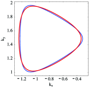
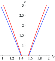
Figure 4: Color online. (a) Non-interacting (blue) and interacting (red) Fermi lines around the $\bf{K}$ point for a doped graphene layer with $\mu\approx 2.4$eV due to the exchange self-energy. The origin of the coordinate system is at the $\Gamma$ point of the BZ. (b) Bare (blue) and renormalized (red) bands for $\mu=0.5$eV.

The self-energy effects are more noticeable in the band slope, as can be observed in Fig.4, where the dispersion relation, calculated without and including the self-energy corrections, is shown. The exchange self-energy enhances the velocity of the bands by a $20\%$ for the used parameter values ($V=t=2.82$eV), renormalizing the kinetic energy. The enhancement of the velocity has been obtained Sarma et al. (2007a); González et al. (1999); Barlas et al. (2007); Polini et al. (2007) previously. Calculating the self-energy within the on-shell approximation, a renormalization of the the velocity compatible with Fermi liquid behavior was obtained for doped graphene Sarma et al. (2007a). The increase of the velocity in lightly-doped graphene has been attributed to the loss in exchange energy when crossing the Dirac point, switching the quasiparticle chirality, by evaluating exchange and RPA correlation energiesBarlas et al. (2007); Polini et al. (2007). All these theoretical works are based on the massless Dirac model for the low-energy excitations of graphene. We find that the exchange energy effects on the FS topology are small for doped graphene, in good agreement with the ARPES results about the evolution of the graphene FS shape with dopingZhou et al. (2006); McChesney et al. (2007).

III.2 Corrections induced by a local interaction

In this section we analyze the corrections induced by a local interaction. The real part of the self-energy is computed from Eq.(18) which gives the second order perturbation theory renormalization of the Green’s function. As explained in Ref.Roldán et al. (2006) this electron-electron interaction self-energy depends on local features of the non-interacting FS, as the Fermi velocity and the curvature of the Fermi line. We limit ourselves to the weak coupling regime as seems generally accepted for graphene, and where the perturbation approach is justified. In Fig.5 the Fermi surfaces, at two different doping levels, have been represented around the corner K of the BZ. It should be notice that the K’ counterpart has to be considered, (see Fig.2 where the hexagonal BZ is represented) in order to include all the possible scattering channels.

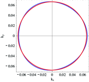
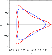
Figure 5: Color online. (a) Non-interacting (blue) and interacting (red) Fermi lines around the $\bf{K}$ point for a doped graphene layer with $\mu\approx 0.2$eV due to a local Coulomb repulsion. (b) Same as (a) but for $\mu\approx 2.4$ eV. Notice the different scales of the coordinate axes. The origin of the coordinate system for this case is placed at the $\bf K$ point.

At low doping, for $\mu\approx 0.2$eV corresponding to a doping density of about $3.9\times 10^{12}$ electrons per cm², the FS has a circular shape and the correction found is small but appreciable. The correction depends on $\vec{\bf k}$, as shown in Fig.5. By increasing the doping level the FS adopts the round triangular shape. At a doping density of $n\approx 6\times 10^{14}$ per cm², corresponding to a chemical potential of $\mu\approx 2.4$eV, the effects of the self-energy are noticeable, and present a strong anisotropy. The deformation of the Fermi surface is maximum along the $\bf{KM}$ direction of the BZ, as can be observed in Fig.5. The topology of the FS is changed by the correction to a concave shape. The underlying hexagonal symmetry ($2\pi/3$ rotation around $\Gamma$ point) is preserved. This correction, with a maximum along the $\bf{KM}$ direction, is consistent with the Renormalization Group analysis inGonzález et al. (1996b), which shows that the Van Hove point defines a stable fixed point, so that interactions deform the Fermi surface towards the saddle point in the band dispersion. Surprising enough, this deformation, induced by pure electron-electron interaction self-energy, presents a strong similarity with the deformation found by ARPES McChesney et al. (2007) in graphene. On Fig.3(a) from Ref.McChesney et al. (2007) the plot of the Fermi contours derived from curvefitting the data, obtained at various dopings, are presented. The anisotropic deformation of the Fermi contours are attributed to electron-phonon coupling to the graphene in-plane optical vibrations. The electron-phonon coupling constant $\lambda_{\pi}(\vec{\bf k})$ extracted from experimental data shows a strong anisotropy (around 5:1 ratio at highest doping) and a much higher strength than would be expected for $\pi$-bands and optical phonons in graphene. It is argued that the abruptness of the kink (change of the band velocity) and the broadening of the bands suggest a strong mass renormalization by electron-phonon coupling. The divergence of $\lambda_{\pi}(\vec{\bf k})$ along the $\bf{KM}$ direction is explained as due to the VHS along the $\bf{KMK}$ boundary line of the BZ, which is reached upon further doping McChesney et al. (2007). The discrepancy between the experimental and theoretical electron-phonon coupling constants has been addressed in ref. Calandra and Mauri (2007a) by using electron-phonon matrix elements extracted from density functional theory simulations. It was found that, including finite resolution effects, the discrepancy between theory and experiment was reduced from a factor of 5.5 to 2.2.

The presence of the strong VHS reveals some similarity to the cupratesDessau et al. (1993). The similarities between graphene and the cuprates have been already remarked by Bena and KivelsonBena and Kivelson (2005) not only because of the VHS but as well because of the similarity between the band structure of graphite and that of the nodal quasiparticles in the cuprate superconductors. The existence of an extended VHS, as probed by the flatness of the bands in both graphene and cuprates, is important because of its effects on the divergences of the density of states. The VHS is related with the interactions which can be enhanced in its proximity and could increase the superconducting critical temperature McChesney et al. (2007), in both cuprates and in graphite intercalated compounds, when $E_{F}$ is placed at the VHS.

In our calculated self-energy, considering only a weak local electron interaction, the proximity to the VHS enhances its correction and it reaches its maximum at the Van Hove band filling, where the Fermi level reaches the VHS ($\mu=t$). Therefore, at low doping, when the FS lies very close to the $\bf K$ point, the corrections to the FS shape are very small since the circular line lies far from the VHS location. On the other hand, at higher doping the Fermi line lies close to the VHS, specially the vertices of the triangle, and therefore the deformation is higher in these directions. In Ref.McChesney et al. (2007) by studying the evolution of the coupling parameter $\lambda_{\pi}(\vec{\bf k})$ with the doping level it is found that, while the minimum coupling strength grows only slowly with doping, the maximum coupling parameter diverges as the corresponding segment of the Fermi contour approaches the VHS at the M point.

The corrections induced by the self-energy calculated from Eq.(18) depend on local features of the non-interacting FS such as the Fermi velocity $v_{F}$ and the curvature of the Fermi line. The main self-energy effects in the square lattice were found to occur when the FS reaches the border of the BZ, where the real part of the self-energy presents pronounced dips close to the saddle points because the $v_{F}$ vanishes at the VHSRoldán et al. (2006). The same behavior is found here for the honeycomb lattice.

Because of the relation between the real and imaginary part of the self-energy, a large self-energy correction to the FS implies a large quasiparticle decay rate in the vicinity that region.

IV Discussion and Concluding Remarks

We have calculated the corrections induced by electron-electron interactions in the band structure of graphene. We limit ourselves to the weak coupling regime, as it is generally assumed to be appropriate for graphene. At first order and zero temperature, the exchange self-energy induces a deformation which contrarest the trigonal warping of the Fermi surface of moderately doped graphene, in agreement with one-loop renormalization group calculations Aleiner et al. (2007). The self-energy corrections round the triangular shape. We find that the effect of the long-range Coulomb repulsion is stronger at low dopings, when the Fermi level lies near the Dirac point. Due to the circular shape of the FS at these fillings, the corrections to the Fermi surface topology are small and only a renormalization of the chemical potential is relevant at this level. On the other hand, the Fermi velocity is enhanced.

The self-energy calculated by second-order perturbation theory, considering a local Hubbard interaction, shows a strong $\vec{\bf k}$-dependence, therefore the deformation induced in the FS topology is anisotropic. The deformation is highest in the $\bf{KM}$ direction of the BZ, and the maximum value is reached near the Van Hove filling, when the Fermi level is very close to the VHS ($\bf M$ point in Fig.1). This deformation of the FS shape appears to be consistent with the anisotropic deformation found by ARPES attributed to a coupling to the graphene in-plane optical phononsMcChesney et al. (2007). A different origin is proposed in Calandra and Mauri (2007b), where the large and anisotropic values of the apparent electron-phonon coupling measured by ARPES in graphene samples doped with K and Ca McChesney et al. (2007), are explained by the strong non-linearity in one of the $\pi^{*}$ bands below E_F due to its hybridization with the dopant Ca atomsCalandra and Mauri (2007b). In the present work, it is induced by a purely electronic interaction. The difficulties in the determination of the origin of some features of the ARPES spectra have been discussed on a theoretical basis in ref. Calandra and Mauri (2007a).

We now comment on the connection between our work and recent theoretical work on correlation effects on graphene. Most of the calculations of the self-energy Sarma et al. (2007a); González et al. (1999); Barlas et al. (2007); Polini et al. (2007) have been carried out for undoped or lightly doped graphene, in the continuum limit, where the conical shape of the bands holds. The effect of the graphene lattice has been included in a recent calculation of the self-energy within the renormalized-ring-diagram approximationYang and Ting (2007). Both doped and undoped graphene present an imaginary part of the self-energy that, near the chemical potential, varies as quadratic in the energy concluding that electrons in graphene behave like a moderately correlated Fermi liquidYang and Ting (2007).

The role of electron-electron interactions in ARPES spectra of graphene has been investigated within the RPA and it is shown to be important on the $vk_{F}$ scale Polini et al. (2007) suggesting that, varying the carrier density, the effects of electron-electron interaction can be separated from electron-phonon interaction effects. The anisotropy of graphene energy-constant maps in ARPES has been proposed to characterize quasiparticle properties Mucha-Kruczynski et al. (2007) from the electronic chirality on monolayer graphene to the magnitude and sign of the interlayer coupling on bilayer graphene. Information about substrate-induced asymmetry may also be extracted from ARPES constant energy patternsMucha-Kruczynski et al. (2007).

Due to the high potential of photoemission to characterize graphene samples, the knowledge of the many-body effects is crucial to interpret some feature in the experimental spectra. The topology of the Fermi surface is related with fundamental properties of the material. To keep track of the different factors involved in the experimental data is needed when comparing theory and experiment. As far as we know, corrections to the FS topology of 2D doped graphene, the main focus of the present work, have not been specifically addressed so far. We conclude that our results highlight the importance of electronic correlation in graphene.

Acknowledgments. Funding from MCyT (Spain) through grants FIS2005-05478-C02-01 and from the European Union Contract No. 12881 (NEST) is acknowledged. We are grateful to E. Rotenberg for illuminating discussions. RR appreciates useful conversations with A. Cortijo.

Appendix A Coulomb interaction between nearest neighbor atoms in the honeycomb lattice.

The Coulomb interaction between electrons in nearest-neighbor atoms in graphene has the form

$$V(\vec{\bf r}_{i}-\vec{\bf r}_{j})=\left\{\begin{array}[]{cc}V=\frac{e^{2}}{a}&\,\,\,{\rm if}\,\,\,|\vec{\bf r}_{i}-\vec{\bf r}_{j}|=a\\ 0&\,\,\,\,\,\,{\rm otherwise}\\ \end{array}\right.$$ (19)

where $\vec{\bf r}_{i,j}$ stand for lattice vectors in the two distinct A and B sites of the honeycomb lattice. Each atom of the sublattice A have three nearest neighbor atoms in the sublattice B, and viceversa, $\vec{\bf r}_{j}=\vec{\bf r}_{i}+\vec{\boldsymbol{\tau}}_{j}$, where $\vec{\boldsymbol{\tau}}_{j}$ are vectors connecting nearest-neighbors sites on the sublattice B from the sublattice A (see Fig.1). The nearest-neighbor interaction term of the Hamiltonian is given by (we omit spin indices)

$${\cal H}_{V}=\frac{1}{2}\sum_{\vec{\bf R}}\sum_{j=1}^{3}V{\hat{b}}^{\dagger}_{\vec{\bf R}+\vec{\boldsymbol{\tau}}_{j}}{\hat{a}}^{\dagger}_{\vec{\bf R}}{\hat{a}}_{\vec{\bf R}}{\hat{b}}_{\vec{\bf R}+\vec{\boldsymbol{\tau}}_{j}}$$ (20)

where $\vec{\bf R}=n_{1}\vec{\bf a}_{1}+n_{2}\vec{\bf a}_{2}$ is the position of an A atom in the lattice, with $n_{1,2}$ integer numbers. The above operators in the momentum space are expressed as

$${\hat{a}}^{\dagger}_{\vec{\bf R}} = \frac{1}{\sqrt{N}}\sum_{\vec{\bf k}\in BZ}e^{-i\vec{\bf k}\cdot\vec{\bf R}}{\hat{a}}^{\dagger}_{\vec{\bf k}}$$

$${\hat{b}}^{\dagger}_{\vec{\bf R}+\vec{\boldsymbol{\tau}}_{j}} = \frac{1}{\sqrt{N}}\sum_{\vec{\bf k}\in BZ}e^{-i\vec{\bf k}\cdot(\vec{\bf R}+\vec{\boldsymbol{\tau}}_{j})}{\hat{b}}^{\dagger}_{\vec{\bf k}}$$

where $N$ is the number of unit cells. The nearest-neighbor Coulomb interaction is found to be

$${\cal H}_{V} = \frac{V}{2}\sum_{j=1}^{3}\sum_{\begin{subarray}{c}\vec{\bf k}\end{subarray},\vec{\bf p},\vec{\bf q}\in BZ}e^{i\vec{\bf q}\cdot\vec{\boldsymbol{\tau}}_{j}}{\hat{b}}^{\dagger}_{\vec{\bf k}}{\hat{a}}^{\dagger}_{\vec{\bf p}}{\hat{a}}_{\vec{\bf p}-\vec{\bf q}}{\hat{b}}_{\vec{\bf k}+\vec{\bf q}}$$

$$= \frac{V}{2}\sum_{\begin{subarray}{c}\vec{\bf q}\end{subarray}\in BZ}f(\vec{\bf q}){\hat{\rho}}^{A}_{-\vec{\bf q}}{\hat{\rho}}^{B}_{\vec{\bf q}}$$

where $f(\vec{\bf q})=\sum_{j=1}^{3}e^{i\vec{\bf q}\cdot\vec{\boldsymbol{\tau}}_{j}}$ and the sublattice density operators are defined as ${\hat{\rho}}_{\vec{\bf q}}^{A}=\sum_{\vec{\bf k}\in BZ}{\hat{a}}^{\dagger}_{\vec{\bf k}+\vec{\bf q}}{\hat{a}}_{\vec{\bf k}}$ (an equivalent definition for ${\hat{\rho}}_{\vec{\bf q}}^{B}$). The operators given in Eq.(A) are related to the creation operators in the subband basis by the rotation ${\hat{c}}^{\dagger}_{\vec{\bf k},\lambda}=1/\sqrt{2}\left(e^{-i\theta_{\vec{\bf k}}/2}{\hat{a}}^{\dagger}_{\vec{\bf k}}+\lambda e^{i\theta_{\vec{\bf k}}/2}{\hat{b}}^{\dagger}_{\vec{\bf k}}\right)$. In this basis, the interacting Hamiltonian can be written as

$${\cal H}_{V}=\sum_{\lambda,\lambda^{\prime}=\pm}\sum_{\begin{subarray}{c}\vec{\bf q}\end{subarray}\in BZ}V^{sr}(\vec{\bf q}){\hat{\rho}}^{\lambda}_{-\vec{\bf q}}{\hat{\rho}}^{\lambda^{\prime}}_{\vec{\bf q}}$$ (23)

with the expression given in Eq.(10) for $V^{sr}(\vec{\bf q})$. Note that, in addition, the overlap matrix elements of the electronic wave-functions must be taken into account in the computation of the exchange self-energy.

Appendix B Integral in momentum space.

In order to calculate the exchange self-energy from Eq.(13) we carry out a momentum integral in the first Brillouin zone. We divide the BZ in two different regions as shown in Fig.6. The long-range interaction dominates in the central region while the nearest-neighbor interaction is important in the outer region of the BZ. The circle centered in $\Gamma$, $0\leq|\vec{\bf q}|\leq\frac{1}{3}\frac{\pi}{\sqrt{3}a}$ is the boundary between the two regions.

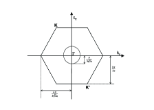
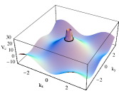
Figure 6: (a) Integration regions in the hexagonal Brilluoin zone. (b) Schematic plot of the Coulomb potential used in the calculation. The black circle separates the inner region where the long-range interaction is dominant from the outer region where the short range-interaction dominates.

The interpolated potential considered in the calculation is schematically plotted in Fig.6. The total potential, resulting from the combination of the long and short range interactions, is a continuous function consistent with the lattice symmetry.

References

- Novoselov and Geim (2004) K. Novoselov and A. Geim, Science 306, 666 (2004).
- Novoselov et al. (2005) K. S. Novoselov, A. K. Geim, S. V. Morozov, D. Jiang, M. Katsnelson, I. Grigorieva, S. Dubonos, and A. Firsov, Nature 438, 197 (2005).
- Zhang et al. (2005) Y. Zhang, Y.-W. Tan, H. Stormer, and P. Kim, Nature 438, 201 (2005).
- Wallace (1947) P. R. Wallace, Phys. Rev. 71, 622 (1947).
- Neto et al. (2007) A. H. C. Neto, F. Guinea, N. M. R. Peres, K. S. Novoselov, and K. A. Geim (2007), eprint arXiv:0709.1163.
- Damascelli et al. (2003) A. Damascelli, Z. Hussain, and Z.-X. Shen, Rev. Mod. Phys. 63, 473 (2003).
- Kopelevich and Esquinazi (2007) Y. Kopelevich and P. Esquinazi, Adv. Mater. (Weinheim, Ger.) 19, 4559 (2007).
- Zhou et al. (2005) S. Y. Zhou, G. H. Gweon, C. D. Spataru, J. Graf, D.-H. Lee, S. G. Louie, and A. Lanzara, Phys. Rev. B 71, 161403(R) (2005).
- Zhou et al. (2006) S. Y. Zhou, G. H. Gweon, J. Graf, A. V. Fedorov, C. D. Spataru, R. D. Diehl, Y. Kopelevich, D. H. Lee, S. G. Louie, and A. Lanzara, Nature Physics 2, 595 (2006).
- Sugawara et al. (2007) K. Sugawara, T. Sato, A.Souma, T. Takahashi, and H. Suematsu, Phys. Rev. Lett. 98, 036801 (2007).
- Xu et al. (1996) S. Xu, J. Cao, C. C. Miller, D. A. Mantell, R. J. D. Miller, and Y. Gao, Phys. Rev. Lett. 76, 483 (1996).
- Moos et al. (2001) G. Moos, C. Gahl, R. Fasel, M. Wolf, and T. Hertel, Phys. Rev. Lett. 87, 267402 (2001).
- González et al. (1996a) J. González, F. Guinea, and M. A. H. Vozmediano, Phys. Rev. Lett. 77, 3589 (1996a).
- Spataru et al. (2001) C. D. Spataru, M. A. Cazalilla, A. Rubio, L. X. Benedict, P. M. Echenique, and S. G. Louie, Phys. Rev. Lett. 87, 246405 (2001).
- López-Sancho et al. (2007) M. P. López-Sancho, M. A. H. Vozmediano, and F. Guinea, Eur. Phys. J. Special Topics 148, 73 (2007).
- Grüneis et al. (2008) A. Grüneis, C. Attaccalite, T. Pichler, V. Zabolotnyy, H. Shiozawa, S. L. Molodtsov, D. Inosov, A. Koitzsch, M. Knupfer, J. Schiessling, et al., Phys. Rev. Lett. 100, 037601 (2008).
- Bostwick et al. (2007) A. Bostwick, T. Ohta, T. Seyller, K. Horn, and E. Rotenberg, Nature Physics 3, 36 (2007).
- McChesney et al. (2007) J. L. McChesney, A. Bostwick, T. Ohta, K. V. Emtsev, T. Seyller, K. Horn, and E. Rotenberg (2007), eprint arXiv:0705.3264.
- Bena and Kivelson (2005) C. Bena and S. A. Kivelson, Phys. Rev. B 72, 125432 (2005).
- González et al. (1993) J. González, F. Guinea, and M. A. H. Vozmediano, Nucl. Phys. 406, 771 (1993).
- Zhou et al. (2007) S. Y. Zhou, G. H. Gweon, A. V. Fedorov, P. First, W. de Heer, D.-H. Lee, F. Guinea, A. C. Neto, and A. Lanzara, Nature Materials 6, 770 (2007).
- Hwang et al. (2007) E. H. Hwang, B. Y.-K. Hu, and S. D. Sarma, Physical Review B 76, 115434 (2007).
- Sarma et al. (2007a) S. D. Sarma, E. H. Hwang, and W.-K. Tse, Phys. Rev. B 75, 121406 (2007a).
- González et al. (1999) J. González, F. Guinea, and M. A. H. Vozmediano, Phys. Rev. B 59, R2474 (1999).
- Barlas et al. (2007) Y. Barlas, T. Perg-Barnea, M. Polini, R. Asgari, and A. H. MacDonald, Phys. Rev. Lett. 98, 236601 (2007).
- Polini et al. (2007) M. Polini, R. Asgari, G. Borghi, Y. Barlas, T. Pereg-Barnea, and A. MacDonald (2007), eprint arXiv:0707.4230v1.
- Mishchenko (2007) E. G. Mishchenko, Phys. Rev. Lett. 98, 216801 (2007).
- Sarma et al. (2007b) S. D. Sarma, B. Y.-K. Hu, E. H. Hwang, and W.-K. Tse (2007b), eprint arXiv:0708.3239.
- Blinowski et al. (1980) J. Blinowski, N. H. Hau, C. Rigaux, J. P. Vieren, R. L. Toullec, G. Furdin, A. Herold, and J. Melin, J. Phys. (Paris) 41, 47 (1980).
- Sorella and Tosatti (1992) S. Sorella and E. Tosatti, Europhys. Lett. 19, 699 (1992).
- Tchougreeff and Hoffmann (1992) A. L. Tchougreeff and R. Hoffmann, J. Phys. Chem. 96, 8993 (1992).
- López-Sancho et al. (2001) M. P. López-Sancho, M. C. Muñoz, and L. Chico, Phys. Rev. B 63, 165419 (2001).
- Perfetto et al. (2002) E. Perfetto, G. Stefanucci, and M. Cini, Phys. Rev. B 66, 165434 (2002).
- Herbut (2006) I. F. Herbut, Phys. Rev. Lett. 97, 146401 (2006).
- Herbut (2007) I. F. Herbut, Phys. Rev. Lett. 99, 206404 (2007).
- Shung (1986) K. W. K. Shung, Phys. Rev. B 34, 979 (1986).
- Lin et al. (1997) M. F. Lin, C. S. Huang, and S. Chuu, Phys. Rev. B 55, 13961 (1997).
- Hwang and Sarma (2007) E. H. Hwang and S. D. Sarma (2007), eprint arXiv:0708.1133v1.
- Wunsch et al. (2006) B. Wunsch, T. Stauber, F. Sols, and F. Guinea, New Journal of Physics 8, 318 (2006).
- Roldán et al. (2006) R. Roldán, M. P. López-Sancho, F. Guinea, and S.-W. Tsai, Europhysics Letters 76, 1165 (2006), ; Phys. Rev. B 74, 235109 (2006).
- (41) The carrier density, for a given chemical potential, is calculated from where is the unit cell area and is the density of states at the energy . Our calculated values of doping densities and corresponding , are in good agreement with the experimental data of the electron density reported for graphene chemically doped by potasium adsorption in Ref.Bostwick et al., 2007 where, for the carrier density is of per cm2 and we found an electron density of per cm2 for the same value of .
- Aleiner et al. (2007) I. L. Aleiner, D. E. Kharzeev, and A. M. Tsvelik, Phys. Rev. B 76, 195415 (2007).
- González et al. (1996b) J. González, F. Guinea, and M. A. H. Vozmediano, Europhys. Lett. 34, 711 (1996b).
- Calandra and Mauri (2007a) M. Calandra and F. Mauri, Phys. Rev. B 76, 205411 (2007a).
- Dessau et al. (1993) D. S. Dessau, Z.-X. Shen, D. M. King, D. S. Marshall, L. W. Lombardo, P. H. Dickinson, A. G. Loeser, J. DiCarlo, C.-H. Park, A. Kapitulnik, et al., Phys. Rev. Lett. 71, 2781 (1993).
- Calandra and Mauri (2007b) M. Calandra and F. Mauri, Phys. Rev. B 76, 161406 (2007b).
- Yang and Ting (2007) X.-Z. Yang and C. S. Ting (2007), eprint arXiv:0705.2752.
- Mucha-Kruczynski et al. (2007) M. Mucha-Kruczynski, O. Tsyplyatyev, A. Grishin, E. McCann, and V. Fal’ko (2007), eprint arXiv:0711.1129.