A transient low-frequency QPO from the black hole binary GRS 1915+105

Abstract

We present the results of the timing analysis of five Rossi X-ray Timing Explorer observations of the Black Hole Candidate GRS 1915+105 between 1996 September and 1997 December. The aim was to investigate the possible presence of a type-B quasi-periodic oscillation (QPO). Since in other systems this QPO is found to appear during spectral transitions from Hard to Soft states, we analyzed observations characterized by a fast and strong variability, in order to have a large number of transitions. In GRS 1915+105, transitions occur on very short time scales ($\sim$ sec): to single them out we averaged Power Density Spectra following the regular path covered by the source on a 3D Hardness-Hardness-Intensity Diagram. We identified both the type-C and the type-B quasi-periodic oscillations (QPOs): this is the first detection of a type-B QPO in GRS 1915+105. As the spectral transitions have been associated to the emission and collimation of relativistic radio-jets, their presence in the prototypical galactic jet source strengthens this connection.

1 Introduction

Systematic variations in the energy spectra and intensity of transient Black-Hole Candidates (BHC) have been recently identified in terms of the pattern described in an X-ray Hardness-Intensity diagram (HID, see Homan et al. 2001, Homan et al. 2005b, Belloni et al. 2005). Four main bright states (in addition to the quiescent state) have been found to correspond to different branches/areas of a square-like HID pattern. In this framework much importance is given to the intermediate states (called Hard Intermediate State, HIMS, and Soft Intermediate State, SIMS) and to the transitions between them, identified from the behaviour in several bands of the electromagnetic spectrum (from radio to hard X-rays, see also Fender, Belloni & Gallo 2004 and Homan et al. 2005b) and from the timing properties of the X-ray light curve.

Low-frequency Quasi-Periodic Oscillations (LFQPOs) with centroid frequency ranging from mHz to tens of Hz have been observed in the X-ray flux of many galactic BHCs since the ’80s (see van der Klis 2006; McClintock & Remillard 2006 and references therein). Three main types of LFQPOs, dubbed Type-A, -B and -C respectively, originally identified in the light curve of XTE J1550-564 (Wijnands et al. 1999; Remillard et al. 2002), have been seen in several sources (see Casella et al. 2005 and references therein). We summarize their properties in Table 1.

In the context of the state classification outlined above, it is possible to ascribe the three LFQPOs to different spectral conditions (see Table 1, Homan et al. 2001, Homan & Belloni 2005, Belloni et al. 2005).

The type-C QPO is associated to the (radio loud) HIMS and to the low/hard state. It is a common QPO seen in almost all BHCs with a variable centroid frequency correlated with the count rate, a high fractional variability and a high coherence ($Q=\nu/$FWHM$\sim$10).

The type-B QPO has been seen only in few systems, although it is being seen in a growing number of sources (see Casella et al. 2005 and references therein). It is a transient QPO associated to spectral transitions from the (radio loud) HIMS to the (radio quiet) SIMS. Its features are a $\sim$ fixed centroid frequency (around $\sim$6 Hz), lower fractional variability and $Q$ than type-C. Some authors (Fender, Belloni & Gallo 2004; Casella et al. 2004) suggested that these spectral transitions are in turn associated to the emission and collimation of transient superluminal relativistic jets visible in radio band. These jets are seen in a number of sources (GRS 1915+105, XTE J1550-564, GX 339-4, XTE J1859+226, GRO J1655-40, etc.). However, not in all of these sources we could resolve the spectral transition to see the transient QPO.

Table 1: Summary of type-A, -B and -C LFQPOs properties (from Casella et al. 2005).

Properties	Type-C	Type-B	Type-A
Frequency (Hz)	$\sim 0.1-15$	$\sim 5-6$	$\sim 8$
Q($\nu/$FWHM)	$\sim 7-12$	$\gtrsim 6$	$\lesssim 3$
Amplitude (% rms)	3-16	$\sim 2-4$	$\lesssim 3$
Noise	strong flat-top	weak red	weak red
Phase laga @$\nu_{QPO}$	soft$/$hardb	hard	soft
Phase lag @2$\nu_{QPO}$	hard	soft	…
Phase lag @$\nu_{QPO}/2$	soft	soft	…

• With “hard lag” we mean that hard variability lags the soft one.

• Trend towards soft lags for increasing QPO frequencies

The spectral properties connected to type-A QPO are similar to those introduced for the type-B. This QPO has been seen in few systems (Casella et al. 2005). It is broader, weaker and less coherent than the type-B QPO.

GRS 1915+105 is a transient BHC discovered on August 15 1992 with the WATCH instrument on board GRANAT (Castro-Tirado et al. 1992, 1994). It is the first galactic source observed to have apparently superluminal transient relativistic radio jets (Mirabel & Rodriguez 1994), commonly interpreted as ejection of ultra-relativistic plasma, with a speed close to the speed of light (up to $\sim 98$%). Its radio variability was discovered to correlate with the hard X-ray flux (Mirabel et al. 1994). Thanks to VLA-radio observations of these jets, Rodriguez et al. (1995) estimated a distance of 12.5 kpc; more recent estimates attest a distance of $6.5\pm 1.6$ kpc (Kaiser et al. 2005). The mass of the compact object was estimated through IR spectroscopic studies (Greiner, Cuby & McCaughrean 2001, Harlaftis & Greiner 2004) to be $14.0\pm 4M_{\odot}$ which unambiguously makes GRS 1915+105 a BHC.

The various and rich phenomenology of this source was classified by Belloni et al. (2000): they analyzed 163 RXTE observations, showing that the complex behaviour of GRS 1915+105 can be described in terms of spectral transitions between three basic states, A, B and C (not to be confused with the name of the LFQPOs introduced before), that give rise to 12 variability classes. The non standard behaviour of GRS 1915+105 (it is a very bright transient source continuing the same outburst started in 1992) was interpreted as that of a source that spends all its time in Intermediate States (both in its hard and soft flavors), never reaching the LS or the quiescence (see e.g. Fender & Belloni, 2004).

GRS 1915+105 also shows strong time variability on time scales of fractions of second, revealing low- and high-frequency QPOs (see Morgan et al. 1997) whose properties (frequency and fractional variability) are tightly correlated with the spectral parameters (Morgan et al. 1997; Muno et al. 1999; Markwardt et al. 1999; Rodriguez et al. 2002a, 2002b; Vignarca et al. 2003). In particular, all LFQPOs observed from this system can be classified as type-C QPOs. Although GRS 1915+105 makes a large number of fast state transitions, which have been positively associated to radio activity and jet ejections, no type-B QPO has been observed to date.

Table 2: Log of the 5 RXTE/PCA observations analyzed in this work

N∘	Obs. Id.	Date	Starting MJD	Exp. (s)	Classification
1	10408-01-35-00	1996 Sep 09	50348.271	9448	$\mu$
2	20402-01-45-03 (#1, 2, 3)	1997 Sep 09	57700.250	10038	$\beta$
3	20402-01-53-00	1997 Oct 31	50752.013	9656	$\beta$
4	20402-01-53-01 & 20402-01-53-02(#1)	1997 Nov 04-05	50756.412	6322	$\mu$
5	20402-01-59-00	1997 Dec 17	50799.091	9784	$\beta$

In this paper we present the discovery with RXTE of the type-B QPO in the X-ray light curve of GRS 1915+105. The QPO was present during fast spectral transitions that we identify with the HIMS to SIMS transition observed in other BHCs.

2 Observations and data analysis

We analyzed five RXTE/PCA observations GRS 1915+105 collected during AO1 and AO2, between 1996 September 22 and 1997 December 17 (see Table 2). We chose observations belonging to variability classes $\mu$ and $\beta$ (according to the classification of Belloni et al. 2000, see Figure 1 for two examples of light curves). Restriction to AO1 and AO2 is due to three reasons: first, AO1 and AO2 observations are those for which a thorough classification was made by Belloni et al. (2000), which removes the need for a complete classification of observations throughout the archive, a task beyond the scope of the present paper; second, AO1 and AO2 were in average characterized by a higher number of working PCUs compared to more recent epochs (this improves the statistics) and third, using data from different epochs, you get different hardness-intensity and color-color diagrams. We chose class $\mu$ and $\beta$ observations because they correspond to intervals when frequent fast transitions among the three spectral states are observed.

Figure 1: 2-13 keV light curves for the two variability classes examined here. Bin size is 1 second.

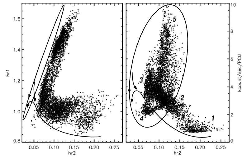
Figure 2: Two-dimensional projections of the hardness-hardness-intensity diagram (HHID) for observation #5. Left side panel: color-color diagram; right side panel: hardness-intensity diagram. Definitions for the colors can be found in §2, the count rate is the 2-13 keV energy band. The arrows follow the source’s regular and repetitive movement. Numbers correspond to the regions discussed in the text (see Figure 3).

The rationale behind this choice was to analyze a large number of spectral transitions from hard (C) to soft states (A and B), when a type-B QPO would be expected. The transitions being fast, the QPO would not be detected for a single transition, but adding a large number of data corresponding to the same transition, the signal could become detectable. The total amount of usable exposure was 44648 seconds. For each observation we produced light curves in the PCA energy channels 0-35 (corresponding to the energy range 2-13 keV) and two color curves defined as the ratio between the counts in the 5-13 and 2-5 keV bands (HR1, absolute channels 14-35 and 0-13) and between the counts in the 13-38 and 2-5 keV bands (HR2, absolute channels 36-103 and 0-13). The bin size was 2 seconds for all these curves. Given the high count rates we did not subtract the background. In addition, for each 2-second time interval we accumulated a power density spectrum (PDS) in the 2-5 keV, 5-13 keV and 13-38 keV energy ranges. All the PDS were extracted with a time resolution of $1/128$ s (corresponding to a Nyquist frequency of 64 Hz). The PCA data modes used to produce the PDS were Binned and Event Data. For an explanation of the different PCA modes see for example Jahoda et al. (1996).

For each observation, we created a 3-dimensional hardness-hardness-intensity diagram (HHID), where the source follows a regular path. For each observation we averaged PDS on a variable number of points ($\sim$100-800, to have enough statistics), following the whole diagram. The selections were made using the free software for multi-variable management XGOBI (http://www.research.att.com/areas/stat/xgobi/). For each selection we rebinned the average PDS logarithmically, and the Poissonian noise, including the Very Large Events (VLE) contribution (Zhang 1995, Zhang et al 1995), was subtracted. The PDS were normalized to square fractional rms (see Belloni & Hasinger 1990) and fitted with a combination of Lorentzians (see Nowak 2000; Belloni et al. 2002). In a few cases (all the PDS of observation #1 and one PDS of observation #3) the Poissonian subtraction left flat residuals at high frequencies, hence we decided to account for it adding an additive constant to the model. The fitting was carried out with the standard XSPEC v11.3 fitting package, by using a one-to-one energy-frequency conversion and a unit response.

For each 2-s interval, we also produced a cross-spectrum between the 2-4.5 keV (absolute channels 0-11) and 4.5-11 keV (absolute channels 12-29) light curves. We then calculated averaged cross-spectrum vectors for all the different selected regions of each observation, from which we derived phase lag spectra (for details on the phase lag analysis see e.g. Casella et al. 2004). We defined phase lags as positive when the hard X-ray variability follows the soft one. In order to quantify the phase-lag information for each detected QPO component we integrated the lags in a range centered on the QPO centroid frequency with a width equal to the FWHM of the QPO peak itself (see Reig et al. 2000). Notice that the estimate of the QPO lags depends on the relative power of the continuum and of the QPO itself. When the continuum power contribution is significantly larger than the QPO power the lags of the continuum may dominate.

3 Results

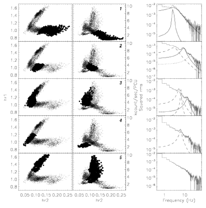
Figure 3: Left panels: Two-dimensional projections of the HHID (see Fig. 2). The tick points mark the five main regions. Right panel: Examples of five corresponding typical power density spectra. For each power spectrum we also plot the best-fit Lorentzian components corresponding to the significant QPOs/bumps ($\sigma\geq 3$). Dashed lines: type-B QPOs, continuous lines: type-C QPOs, dotted lines: harmonics. In the PDS in region 4 the Lorentzian fitting a bump identified as the harmonic of the type-B QPO ($\nu=13.84$ Hz) has not been reported since it has been detected with a significance $\sigma<3$.

Figure 4: Evolution of QPOs/bumps (with significance $\sigma\geq 3$) centroid frequencies as a function of the position in the HHID in Figure 3, for all the analyzed observations. Adopted criteria are explained in the text.

Table 3: QPO types detected in the five regions for all considered observations. Region 1 is not present in observations # 2 and 3. We indicated with “Bump-B” peaks with $Q<2$.

	Regions in figure 3
Obs. #	1	2	3	4	5
1	-	Bump-B, C	C, B	B	No peaks
2	C	C	C, B	No peaks	No peaks
3	C	Bump-B, C	C, B	No peaks	No peaks
4	-	C	C, B	B	No peaks
5	C	Bump-B, C	C, B	B	No peaks

An example of HHID is shown in the two-dimensional projections in Fig. 2 (from observation #5, class $\beta$). The regular and repetitive movement followed by the source is marked by the arrows. Starting from the bottom-right corner of both projections, the PDS properties were found to change smoothly thorough the diagram. We could identify five main average behaviours of the PDS corresponding to five regions in the diagram. In Figure 3 we show the five regions in the two-dimensional projections of the HHID of observation #5, together with five corresponding examples of PDS. In Figure 4 we show the evolution of the frequencies of all significant peaks (with significance $\sigma\geq 3$) for all the observations, moving through the HHID following the arrows in Figure 2. The x axis has been chosen in such a way to have an equal spacing between different selections in the same region, since the same region in different observations has been divided in a different number of selections. This point can be clarified by looking tables 4 to 8 in appendix A, where we reported all the significant peaks different from a continuum fitted in all the selections of the five observations. For each selection (in figure 4) we reported the peak frequency obtained from the energy range where the feature was more significant. In four cases we found that the same feature was detected at more than 3 sigma as a QPO (i.e. with a quality factor $Q\geq 2$) in one energy band and, with a higher significance, as a bump ($Q<2$) in another. In these cases we decided to report the frequency obtained from the QPO. We considered two peaks as harmonics of each other if (i) their centroid frequencies, fitted independently, are consistent with being harmonically related or (ii) fixing their centroid frequency to an harmonic ratio we could obtain a very good fit. We will no longer consider harmonic peaks in our discussion.

In Figure 3 we can easily identify the presence of two peaks evolving in frequency thorough the diagram from region 1 to region 4 (see Table 3 for a summary of their properties):

1. the first peak is detected (superimposed to a broad-band noise) since region 1. It increases in frequency (from $\sim$2 Hz to $\sim$15 Hz) and quality factor $Q$ (from 0.64 to 7.39) and decreases in fractional rms amplitude (from 22.86 to 1.16) while moving thorough the diagram from region 1 to 2 until it disappears at high count rates at the end of region 3. Its fractional rms is higher in the hardest band (13-38 keV);

2. a second peak is detected in region 2 (in three observations, see table 3) with properties markedly different from the first one. It has initially (in region 2) a frequency between 2.44 Hz and 2.84 Hz and a quality factor $Q<2$. In regions 3 and 4 it shows a much less variable frequency than the first peak (slowly increasing from $\sim$4 to 7 Hz) and a $Q>2$. Its fractional rms is higher in the hardest band (13-38 keV), is lower than that of the first peak and is independent on the centroid frequency (see Fig. 5).

All five analyzed observations follow the average behaviour described above, with three main exceptions:

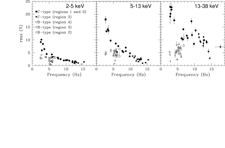
Figure 5: Fractional rms of the detected Bumps/QPOs in all observations as function of their frequency for energy bands 2-5 keV (PCA channels 0-13, left panel), 5-13 keV (PCA channels 14-35, center panel) and 13-38 keV (PCA channels 36-103, right panel). Error bars are estimated at 1 $\sigma$ confidence level. Arrows indicate 3 $\sigma$ upper limits for type-C QPOs only. Filled symbols indicate type-C QPOs, open symbols type-B.

(a) region 1, which correspond to the long hard intervals in the light curve of class $\beta$ (see Fig. 1, upper panel), are not present in the two class $\mu$ observations (#1 and #4). Since this is the main macroscopic difference between the two classes, and since a detailed analysis of the long hard intervals of class $\beta$ light curves is beyond the scope of this work, in the following of the paper we will consider the two classes as a single class.

(b) No QPO is detected in the PDS from region 4 of observations #2 (class $\beta$) and #3 (class $\mu$). In region 4 of observation #3, only in the highest energy band, we find a non-significant QPO ($\sigma$=2.4) with the following properties: $\nu$ = 5.85$\pm$0.26 Hz, $Q$ = 3.21$\pm$2.43, rms = (6.26$\pm$1.35)%. Both the rms amplitude value and the centroid frequency are consistent with those of the peak found in region 4 in the 36-103 keV energy band for observations #1, 4 and 5, but the uncertainty on the quality factor $Q$ and the low significance ($<$3 $\sigma$) does not allow us to claim the real detection of a QPO.

(c) In region 2, we detected two significant peaks in observations # 2, 3 and 5, while just one significant peak in observations #2 and 4. In region 2 of observation #4, we find a non-significant QPO ($\sigma$=2.44) with the following properties (values from 14-35 keV energy band): $\nu$ = 3.46$\pm$0.18 Hz, $Q$ = 2.44$\pm$1.03, rms = (3.68$\pm$0.93)%. Its properties are consistent with those of the low-frequency peak found in region 2 for observations #1, 3 and 5, but the significance ($<$3 $\sigma$) does not allow us to claim the real detection of a QPO.

We will refer to the peak with centroid frequency ranging from $\sim$2 up to 15 Hz as type-C QPO and to the peak with 2.44–7 Hz frequency detected in regions 2, 3 and 4 as type-B QPO. This identification will be motivated below. In Figure 5 we show the fractional rms amplitude of all the detected Bumps/QPOs as a function of their centroid frequency, for each of the three energy bands analyzed. In a few cases QPOs were detected only in one or two energy ranges. In these cases in order to obtain a more reliable estimate of the peak amplitude also in the energy range where it was not significant we fixed its centroid and FWHM to the values obtained from the energy range in which it was more significant.

The points with large errors in frequency correspond to detections where we need two Lorentzian components to obtain a satisfactory fit. For these points we plot the average of the two centroid frequencies with an error estimated as the sum between the two errors (we considered this the most conservative approach possible). In order to check whether these double peaks are due to the frequency variability of the QPO we tried to select smaller regions in the HHID. However we could not detect the QPO in such selections, due to the low statistics of the resulting PDS.

From Figure 3 we can relate the presence of the QPO-types to different zones of the source path in the HHID but we do not have any detailed information about the time evolution of the source position in that diagram. We know that $\mu$ and $\beta$ classes are characterized by fast and strong variability and frequent spectral transitions but we do not know precisely between which spectral states the transitions happen and when. A light curve where parts corresponding to different regions in the HHID are marked with different symbols can help us to clarify this point (see Figure 6). We chose a 300-second interval representative of the source behaviour. With the identifications Downward Triangles = Reg. 1, Circles = Reg. 2, Stars = Reg. 3, Upward Triangles = Reg. 4 and Squares = Reg. 5 we have the following regions sequence: 2345 345 532. Class $\beta$ observations are also characterized by the presence of long hard intervals (region 1), occasionally occurring when the source maps the hard tail in the bottom-right part of both the diagrams in Figure 2, always between region-2 intervals. If, using the state classification presented in Belloni et al. (2000), we make the identifications Reg. 2 = C-state, Reg. 4 = A-state, Reg. 5 = B-state and we consider Reg. 3 as a Transition (T) state, we have the following state sequences: C T AB T AB T C. In this framework region 1 is the hardest part of the C-state.

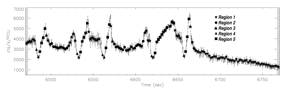
Figure 6: 300-second light curve (2-13 keV energy band) for observation # 5. Bin size is 0.125 sec. Every symbol is averaged on 2 seconds. Different symbols correspond to different regions in the HHID in Figure 3.

3.1 Phase lags

Phase lags for all the detected peaks are reported in Tables 9 and 10 in appendix A. In Figure 7 we show phase lags vs. frequency for the type-C QPO in two observations. If the QPO was fitted with two Lorentzians we estimated the phase lag integrating on a peak centered on the centroid frequency of the Lorentzian with the highest rms amplitude and with the FWHM of the same component. For observation # 1, a negative trend for increasing QPO frequencies is visible, although one point is completely out of this trend. For observation # 5 the phase lag of the QPOs are always negative and consistent with being constant.

In Figure 8 we show two examples of power density spectra (upper panels) and phase-lag spectra (bottom panels) from regions where a type-B QPO was detected. In the left panel (observation #4), even thought the errors on phase lags are large, a turn towards positive lag values in correspondence of the QPO frequency is apparent. However, extracting the phase lags over the whole peak width (i.e. over the frequency range $\nu_{p}\;\pm\;$FWHM/2) we obtain a negative value of the lags (although consistent with zero, $\phi$ = -0.07$\pm$0.05 rad). In the right panel (observation #1) we have a much better statistics and the phase lags are clearly negative ($\phi$ = -0.11$\pm$0.007 rad) in correspondence of the type-B QPO (when integrated over the whole peak width).

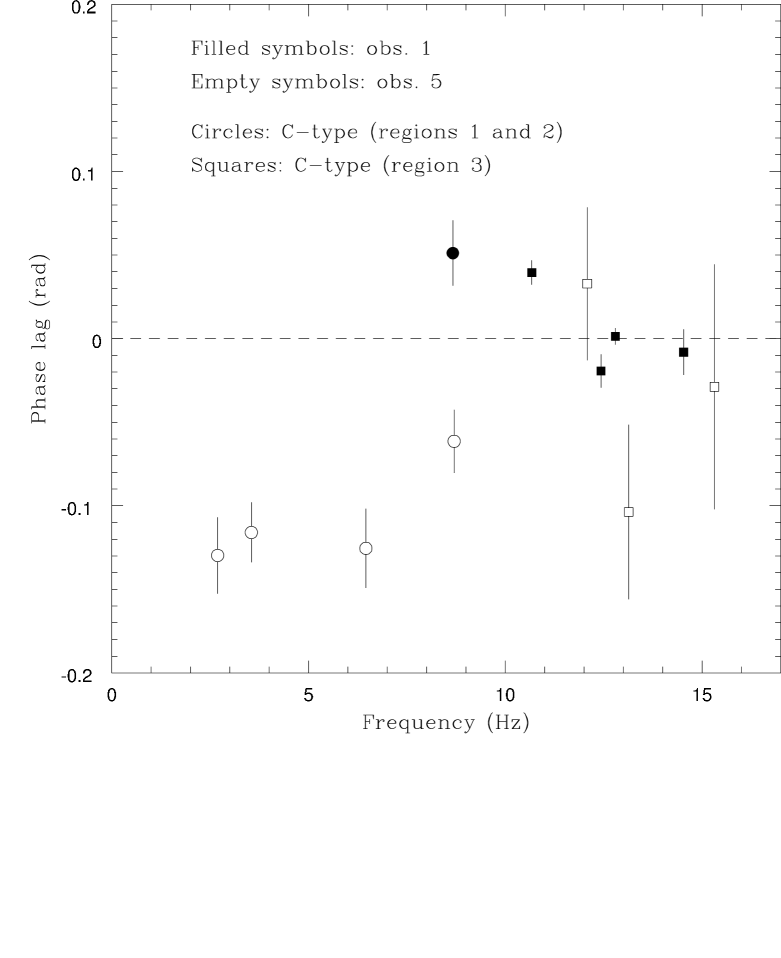
Figure 7: Phase lags of type-C QPOs detected in two representative observations. For each QPO we extracted the phase lag in a range centered at the QPO peak frequency and corresponding to the width itself ($\nu_{p}\,\pm\,FWHM/2$). Errors bar on the X-axis are not shown for clarity.

Figure 8: Power density spectra and phase-lag spectra of two different observations/regions where a type-B QPO was detected. The dashed line marks the QPO frequency, the dotted lines mark $\nu\pm HWHM$. Left panel: type-B QPO detected averaging power spectra (121 points) in region 4 of observation # 5. Right panel: type-B QPO detected averaging power spectra (842 points) in region 3 of observation # 1.

4 Discussion and conclusions

We analyzed 5 RXTE/PCA observations collected during the first two years of the mission. In the power density spectra of all five observations we detected several peaks which we identify with two different types of QPO already seen in many other BHCs: the type-C and type-B QPOs. This is the first identification of a type-B QPO in GRS 1915+105. To detect it, we looked in detail at spectral transitions in observations characterized by a fast and intense variability. Spectral transitions in GRS 1915+105 are usually very fast, often occurring on timescales of $\sim$ seconds. This is at variance with most of other black-hole binaries in which spectral transitions are observed to last hours or days. In order to study the spectral transitions in GRS 1915+105 we performed an energy-dependent timing analysis by averaging power spectra on the pattern the source recursively tracks in the 3-dimensional hardness-hardness-intensity diagram.

Applying this method, we found a type-B QPO in all five observations. In all of them, we detected the type-B QPO together with the type-C, in region # 3 of the HHID (see Tab. 3). In three of them, we also detected a type-B QPO alone, in region # 4 of the HHID. Two of these observations belong to class $\mu$ and one to class $\beta$, which excludes any relation between the class of variability and the presence of the type-B QPO. This means that the presence of the long hard intervals (which differentiate the $\beta$-class from the $\mu$-class light curves) does not influence the fast timing properties of the source outside these intervals. We could not find any property (as e.g. hardness, rate) correlated with the presence of the type-B QPO alone in region 4 of the HHID. In three observations we also found a type-B bump in region 2. No correlations were found neither between the presence of the type-B bump and the type-B QPO in region 4 nor with the hardness and the count rate.

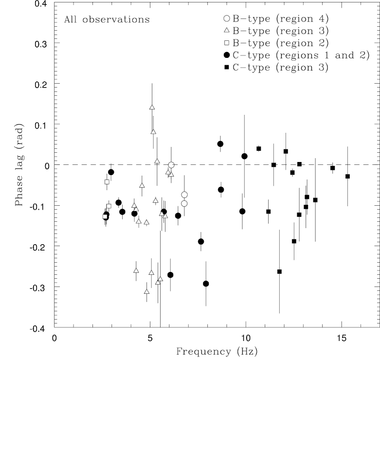
Figure 9: Phase lags of the detected QPOs in all observations. For each QPO we extracted the phase lag in a range centered at the QPO peak frequency and corresponding to the width itself ($\nu_{p}\,\pm\,FWHM/2$). Errors bar on the X-axis are not shown for clarity.

4.1 QPOs identification

In order to identify the two types of QPO that we found in our data sets, we compare them with the known LFQPOs in BHCs. In particular we first analyze their position and behaviour in the Hardness-Intensity diagram (right panel of Figure 2). When the source moves through regions #1 and #2 up to region #3 the first QPO shows a behaviour very similar to that of type-C QPOs: its frequency is correlated with the count rate and is inversely correlated with the hardness. At a certain hardness, this QPO disappears. A second type of QPO is also detected: as in the case of type-B QPOs, this second QPO appears in a narrow frequency range (often around $\sim$6 Hz) and in a limited range in hardness.

Its frequency and quality factor appear to be slightly correlated with the count rate, particularly when at its lowest frequencies (2.44-2.84 Hz). We interpret this as the first evidence of an increase of the coherence of the type-B QPO from $Q<2$ when at low frequencies to $Q>2$ when reaching frequencies around $\sim$6 Hz, possibly suggesting the presence of a resonance at this frequency (see Casella et al. 2004).

The combined evolution of the QPOs in GRS 1915+105 is strongly reminiscent of the known behaviour of type-C and type-B QPOs in BHCs (see Casella et al. 2005 and references therein).

To verify this identification, we plot in Figure 5 the rms fractional variability of the detected QPOs as a function of their frequency for three energy bands. The two QPO types have a somewhat similar energy dependency (being stronger at high energy) but they clearly show different behaviours in these diagrams. In each of the three panels, two well-identified groups of points are evident. A comparison of these two groups with Figure #3 of Casella et al. 2004 helps to classify the observed QPO in GRS 1915+105: the first group is diagonally spread across the plots, covering the whole frequency range between $\sim 2$ and $\sim 15$ Hz and a large range in rms (particularly at high energies, see the right panel of Figure 5). The second group is clustered both in frequency (between $\sim 2.5$ and $\sim 7$ Hz) and in fractional rms. The observed behaviour is clearly consistent with that known to be typical of type-C and type-B QPOs in BHCs (see Casella et al. 2004, 2005).

4.2 Phase lags

The association between QPO-type and phase lag in literature is not conclusive: although an average behaviour can be identified (see Tab. 1, Casella et al. 2005 and reference therein) there are a number of exceptions (see e.g. Belloni et al. 2005 and Homan et al. 2005a). Nevertheless we performed a phase-lag analysis in order to have a comprehensive view of the behaviour of the QPOs in GRS 1915+105.

On the basis of the analyzed data it is not possible to characterize unambiguously the phase lag behaviour of any of the two types of QPO we observe: lags appear to vary between different observations, although both types show in average negative values of phase lag (see Fig. 9).

This can possibly due to the fast variability of the analyzed light curves: we extracted power spectra over time intervals 2 seconds long, without applying any procedure to detrend the variability on longer time scales. However, this variability is very strong (see Fig. 1), which results in a leakage at higher frequencies as strong as to actually dominate the phase-lag continuum.

4.3 GRS 1915+105 as a “normal” source

The type-B QPO was detected in a few BHCs (see Casella et al. 2005), and associated to spectral transitions from HIMS to SIMS (Homan & Belloni 2005, Belloni et al. 2005 and reference therein). Some authors (Gallo et al 2003; Fender, Belloni & Gallo 2004) suggested a relation between these spectral transitions and the emission and collimation of transient relativistic radio jets: if we consider the type-B QPO as the signature of radio jet emission, we have this “signature” also in the prototypical galactic jet source. As already pointed out by Belloni et al. (2005), the non-detection of a type-B QPO in GRS 1915+105 was rather interesting, especially if you interpret the X-ray$/$radio correlation in this source and in other transients in the framework of the same model (Fender, Belloni & Gallo 2004). In GRS 1915+105 the association between X-ray and radio activity is well known (Pooley & Fender 1997, Mirabel et al. 1998, Fender & Belloni 2004 and references therein). Belloni et al. 2005 suggested that the elusiveness of this QPO (in GRS 1915+105) could be due to high velocity of the movement of the source through the HID. The result presented in this work thus strengthens the interpretation of GRS 1915+105 in the framework of the same model of other BHCs: a type-B QPO appears in correspondence of spectral transition from the B-state to the A-state (Transition, Region 3, Stars in Figure 6) and when the source is in the A-state (Region 4, Upward Triangles in Figure 6). In the light curve in Figure 6 we see state oscillations CTAB TAB TAB that we can identify as fast passages between the HIMS and the SIMS of the other BHCs (Casella et al. 2004; Fender, Belloni & Gallo 2004). The type-B QPO appears also in correspondence of the transition from the B-state to the C-state (Squares-Stars-Circles in Figure 6), therefore not in an oscillation event but in a transition from a soft to a hard state.

Furthermore, GRS 1915+105 is at present the heaviest black hole (although uncertainties on BH mass values are rather large, see McClintock & Remillard 2006 and references therein) in which a type-B QPO has been observed at 6 Hz (when its quality factor $Q>2$). This strengthens the already known independence of this type of QPO on the mass of the compact object (see Casella et al. 2005).

4.4 X-ray$/$radio association

Klein-Wolt et al. (2002) made a detailed study of simultaneous radio$/$X-ray observations of GRS 1915+105, focusing in particular on radio oscillation events, and found that $\beta$ class observations are usually associated to strong radio oscillations, while $\mu$ class observations are usually associated to a weak steady radio activity. These authors point out that the long hard intervals (which are the main macroscopic difference between the two variability classes) appear to be directly linked to the production of radio oscillations. We found the type-B QPO in both classes $\beta$ and $\mu$. We could not find any timing property (on time scales shorter than 2 seconds) clearly differentiating the two classes. This apparently weakens the link between the presence of the type-B QPO and radio activity. Unfortunately, the lack of radio coverage during the analyzed RXTE observations does not allow any conclusive result. In order to clarify this issue it will be fundamental to extend our analysis to RXTE observations for which a radio coverage is available.

Appendix A Fit results and phase lags

Here we report five tables containing the fit results for the analysed observations and two tables with the results of the phase lag analysis.

Table 4: Fit results for Obs. #1. We accounted for the Poissonian noise adding an additive constant to the model (see §2). In the first column the bold number indicates the region, the second number indicates the selection within the region and it increases following the arrows in figure 2. For peaks fitted with two Lorentzians, both the components are reported. If the difference between the negative and the positive error was smaller than 0.1, we reported just the value of the largest error (in absolute value). With “Fixed fit” we refer to those cases when QPOs were detected only in one or two energy ranges: in these cases we fixed the centroid frequency and the $FWHM$ to the values obtained from the energy range in which the peak was more significant (see §3).

Observation #1
Sel.	Type	Freq. (Hz)	$FWHM$	Sign. ($\sigma$)	rms ($\%$)
2-5 keV
2-1	B	2.75$\pm$0.16	1.72${}_{-0.36}^{+0.42}$	4.68	4.18$\pm$0.45
2-1	C	9.35$\pm$0.33	1.67${}_{-0.68}^{+1.07}$	3.10	2.04$\pm$0.39
3-1	B	3.99$\pm$0.07	2.21$\pm$0.21	13.26	3.46$\pm$0.13
3-1	C	10.92$\pm$0.32	4.33${}_{-0.73}^{+0.88}$	7.00	2.05$\pm$0.16
3-2	B	5.04$\pm$0.06	2.39$\pm$0.21	16.13	3.15$\pm$0.10
3-2	C	13.09${}_{-0.60}^{+0.48}$	4.10${}_{-1.53}^{+2.12}$	3.45	1.25$\pm$0.23
3-3	B	5.65$\pm$0.09	2.70$\pm$0.27	14.00	3.33$\pm$0.12
3-3	C	12.43	4.39	Fixed fit	0.91$\pm$0.20
3-4	B	6.01$\pm$0.16	2.68$\pm$0.49	8.53	2.06$\pm$0.13
3-4	C	14.53	2.66	Upp. lim.d	0.70
3-5	B	5.94	5.51	Upp. lim.d	1.47
4-1	B	6.39$\pm$0.20	1.99${}_{-0.62}^{+0.91}$	4.48	3.07$\pm$0.41
5-13 keV
2-1	B	2.75	1.72	Fixed fit	5.23$\pm$0.52
2-1	C	8.67$\pm$0.27	5.42${}_{-0.83}^{+0.95}$	7.87	7.02$\pm$0.45
3-1	B	4.27$\pm$0.04	1.84$\pm$0.10	23.23	5.60$\pm$0.12
3-1	C	10.67$\pm$0.10	3.95$\pm$0.27	19.09	3.70$\pm$0.10
3-2	B-1st	4.81$\pm$0.08	1.39$\pm$0.18	5.56	-a
3-2	B-2nd	5.72$\pm$0.06	1.03$\pm$0.11	5.01	5.23$\pm$0.50b
3-2	C	12.80$\pm$0.40	8.92${}_{-1.36}^{+1.56}$	6.74	2.40$\pm$0.18
3-3	B-1st	5.28$\pm$0.12	1.81$\pm$0.20	8.08	-a
3-3	B-2nd	6.34$\pm$0.06	0.82$\pm$0.14	4.48	6.38$\pm$0.52b
3-3	C	12.43$\pm$0.58	4.39${}_{-1.52}^{+2.26}$	3.56	1.58$\pm$0.27
3-4	B	6.10$\pm$0.05	2.32$\pm$0.15	21.58	4.20$\pm$0.10
3-4	C	14.53$\pm$0.35	2.66${}_{-0.72}^{+1.10}$	4.27	1.16$\pm$0.16
3-5	B	5.94${}_{-0.50}^{+0.37}$	5.51${}_{-0.89}^{+1.12}$	6.39	3.42$\pm$0.35
4-1	B	6.78$\pm$0.08	0.63${}_{-0.21}^{+0.80}$	5.43	3.66${}_{-0.34}^{+1.55}$
13-38 keV
2-1	B	2.74	1.72	Upp. lim.d	4.38
2-1	C	9.08$\pm$0.30	4.01${}_{-0.84}^{+0.96}$	7.43	17.25$\pm$1.20
3-1	B	4.27	1.84	Fixed fit	4.92${}_{-0.50}^{+1.35}$
3-1	C	11.24$\pm$0.10	3.53$\pm$0.39	10.91	12.32$\pm$0.56
3-2	B	5.77$\pm$0.15	1.37${}_{-0.42}^{+0.54}$	3.93	4.80$\pm$0.69
3-2	C	12.65$\pm$0.13	2.77${}_{-0.48}^{+0.54}$	5.19	8.70$\pm$0.87
3-2	Cc	17.88${}_{-2.77}^{+3.48}$	19.96${}_{-7.88}^{+0.04}$	3.76	10.12${}_{-1.35}^{+1.58}$
3-3	B	5.65	2.70	Fixed fit	6.82$\pm$0.50
3-3	C	14.53	2.66	Fixed fit	2.89$\pm$0.53
4-1	B	6.78	0.63	Fixed fit	7.83$\pm$0.67

• Peak fitted with two Lorentzians. The value of the rms is reported at the next line

• Sum of the rms of the two Lorentzians fitting this peak

• Harmonic peak

• Estimated at 3$\sigma$ confidence level

Table 5: Fit results for Obs. #2. See caption of Table 6 for an explanation.

Observation #2
Sel.	Type	Freq. (Hz)	$FWHM$	Sign. ($\sigma$)	rms ($\%$)
2-5 keV
1-1	C	2.86$\pm$0.06	1.25$\pm$0.19	6.46	5.94$\pm$0.46
1-1	Cc	4.99$\pm$0.43	3.41$\pm$0.68	4.68	4.36${}_{-0.47}^{+0.69}$
1-2	C	4.27$\pm$0.08	1.77$\pm$0.29	6.99	4.54$\pm$0.42
1-3	C	6.06$\pm$0.13	1.74$\pm$0.33	5.98	3.37$\pm$0.28
2-1	C	7.72$\pm$0.13	1.92$\pm$0.40	7.06	2.77$\pm$0.20
2-2	C	9.98$\pm$0.19	2.98$\pm$0.55	7.11	2.11$\pm$0.15
3-1	B	5.54$\pm$0.15	1.07${}_{-0.28}^{+0.38}$	4.68	1.72$\pm$0.24
3-1	C	12.57${}_{-0.33}^{+0.22}$	1.70${}_{-0.54}^{+0.95}$	3.01	1.24$\pm$0.21
3-2	B	5.10	0.98	Fixed fit	0.83${}_{-0.23}^{+0.63}$
3-2	C	12.72	5.51	Upp. lim.d	0.90
5-13 keV
1-1	C	2.96$\pm$0.58	1.43$\pm$0.13	11.34	13.36$\pm$0.60
1-1	Cc	5.25$\pm$0.61	5.44$\pm$0.61	5.16	8.23${}_{-0.81}^{+1.10}$
1-2	C	4.18$\pm$0.06	2.15$\pm$0.21	11.76	9.73$\pm$0.47
1-3	C	6.06$\pm$0.07	1.25$\pm$0.19	9.75	5.31$\pm$0.31
2-1	C	7.91$\pm$0.06	1.74$\pm$0.16	25.56	5.29${}_{-0.10}^{+0.20}$
2-1	Cc	15.17${}_{-2.18}^{+1.35}$	15.48${}_{-3.62}^{+4.51}$	4.68	3.55${}_{-0.39}^{+0.58}$
2-2	C	9.81$\pm$0.08	2.41$\pm$0.26	14.20	3.62$\pm$0.13
2-2	Cc	21.15$\pm$0.92	7.31${}_{-2.32}^{+3.80}$	4.68	1.68${}_{-0.18}^{+0.32}$
3-1	B-1st	5.75$\pm$0.01	$<$0.5e	8.07	-a
3-1	B-2nd	4.57$\pm$0.10	1.39$\pm$0.23	7.09	4.59$\pm$0.33b
3-1	C	12.78$\pm$0.12	2.1$\pm$50.34	9.09	2.23$\pm$0.13
3-2	B	5.10$\pm$0.10	0.98$\pm$0.21	7.08	3.80$\pm$0.27
3-2	C	11.75$\pm$0.18	1.72${}_{-0.38}^{+0.48}$	5.47	1.83$\pm$0.19
13-38 keV
1-1	C	2.89$\pm$0.06	1.67$\pm$0.21	6.56	20.17$\pm$1.57
1-2	C	4.01$\pm$0.17	3.54$\pm$0.43	6.06	17.62$\pm$1.46
1-3	C	6.55$\pm$0.10	1.59$\pm$0.35	6.02	10.24$\pm$0.85
1-3	Cc	13.19${}_{-2.67}^{+2.26}$	11.33${}_{-3.26}^{+3.66}$	3.37	7.85${}_{-1.18}^{+1.58}$
2-1	C	7.97$\pm$0.13	1.72$\pm$0.39	4.10	10.74${}_{-1.31}^{+1.04}$
2-2	C	9.84$\pm$0.14	1.73$\pm$0.35	5.19	8.47${}_{-0.82}^{+0.93}$
3-1	B	5.16$\pm$0.26	1.07${}_{-0.55}^{+0.68}$	5.45	7.04$\pm$0.71
3-1	C	12.94$\pm$0.18	5.05$\pm$0.33	10.36	9.92$\pm$0.48
3-2	B	4.74$\pm$0.245	1.36${}_{-0.21}^{+0.56}$	6.07	8.10${}_{-0.67}^{+1.40}$
3-2	C	12.72${}_{-0.29}^{+0.43}$	5.51${}_{-1.06}^{+0.86}$	7.07	9.92${}_{-0.71}^{+0.52}$

• Peak fitted with two Lorentzians. The value of the rms is reported at the next line

• Sum of the rms of the two Lorentzians fitting this peak

• Harmonic peak

• Estimated at 3$\sigma$ confidence level

• Our resolution is 0.5 s (we extracted power density spectra on 2-second intervals, see §2)

Table 6: Fit results for Obs. #3. In the first column the bold number indicates the region, the second number indicates the selection within the region and it increases following the arrows in figure 2. For peaks fitted with two Lorentzians, both the components are reported. If the difference between the negative and the positive error was smaller than 0.1, we reported just the value of the largest error (in absolute value). With “Fixed fit” we refer to those cases when QPOs were detected only in one or two energy ranges: in these cases we fixed the centroid frequency and the $FWHM$ to the values obtained from the energy range in which the peak was more significant (see §3).

Observation #3
Sel.	Type	Freq. (Hz)	$FWHM$	Sign. ($\sigma$)	rms ($\%$)
2-5 keV
1-1	C	2.72	2.29	Fixed fit	10.12$\pm$0.35
1-2	C	3.58$\pm$0.09	2.41$\pm$0.28	6.57	6.42$\pm$0.53
1-3	C	5.80$\pm$0.10	1.93$\pm$0.28	8.66	4.36$\pm$0.26
1-3	Cc	13.41${}_{-0.61}^{+0.71}$	5.60${}_{-1.98}^{+3.28}$	3.74	2.48${}_{-0.33}^{+0.45}$
2-1	B	2.44$\pm$0.28	2.24$\pm$0.49	3.06	2.95${}_{-0.48}^{+0.68}$
2-1	C	7.57$\pm$0.07	2.28$\pm$0.24	21.08	3.14$\pm$0.13
2-1	Cc	15.91${}_{-4.00}^{+3.26}$	19.98${}_{-1.42}^{+0.02}$	5.01	2.01 ${}_{-0.20}^{+0.30}$
3-1	B	5.03$\pm$0.33	2.62${}_{-0.61}^{+0.92}$	4.00	1.77${}_{-0.22}^{+0.33}$
3-1	C	11.00$\pm$0.21	3.66${}_{-0.57}^{+0.69}$	6.94	1.84$\pm$0.13
3-2	B	5.91$\pm$0.09	0.71$\pm$0.18	5.46	1.47$\pm$0.13
3-2	C	12.59$\pm$0.27	3.69$\pm$0.84	6.79	1.70$\pm$0.15
3-3	B	5.53	0.75	Fixed fit	0.41$\pm$0.28
3-4a	B	5.37	1.45	Fixed fit	0.51$\pm$0.10
5-13 keV
1-1	C	2.72$\pm$0.14	4.01$\pm$0.23	15.77	18.04$\pm$0.58
1-2	C	3.35$\pm$0.08	2.80$\pm$0.22	8.23	14.13${}_{-0.86}^{+1.03}$
1-3	C	5.71$\pm$0.09	2.13$\pm$0.21	9.09	8.61$\pm$0.47
1-3	Cc	13.90$\pm$0.54	10.36${}_{-1.10}^{+1.23}$	9.81	5.58$\pm$0.31
2-1	B	2.64$\pm$0.21	2.24$\pm$0.38	3.50	4.40${}_{-0.63}^{+0.76}$
2-1	C	7.65$\pm$0.04	1.94$\pm$0.10	24.82	5.74$\pm$0.12
2-1	Cc	14.85${}_{-0.92}^{+0.77}$	15.89${}_{-1.66}^{+1.82}$	9.05	3.88$\pm$0.25
3-1	B-1st	5.77$\pm$0.03	$<$0.5f	6.93	-b
3-1	B-2nd	4.17$\pm$0.12	2.31$\pm$0.41	5.42	4.04$\pm$0.43d
3-1	C	11.17$\pm$0.12	3.89$\pm$0.29	15.98	3.13$\pm$0.10
3-1	-e	25.00${}_{-1.43}^{+1.30}$	9.37${}_{-2.23}^{+3.35}$	3.80	1.27$\pm$0.20
3-2	B-1st	5.17$\pm$0.06	1.00$\pm$0.14	13.78	-b
3-2	B-2nd	6.25$\pm$0.02	$<$0.5f	8.23	3.97$\pm$0.18d
3-2	C	13.19$\pm$0.16	3.66$\pm$0.45	13.39	2.41$\pm$0.11
3-3	B	5.53$\pm$0.05	0.75$\pm$0.23	8.14	1.99$\pm$0.13
3-4a	B	5.36$\pm$0.16	1.45${}_{-0.29}^{+0.45}$	3.90	0.78$\pm$0.10
13-38 keV
1-1	C	2.80$\pm$0.22	3.42$\pm$0.36	8.13	22.86${}_{-1.42}^{+1.54}$
1-2	C	3.20$\pm$0.10	3.18$\pm$0.20	11.42	21.77$\pm$0.96
1-3	C	6.15$\pm$0.07	1.29$\pm$0.30	5.95	10.61$\pm$0.89
2-1	B	2.64	2.24	Fixed fit	5.29$\pm$0.69
2-1	C	7.71$\pm$0.06	1.58$\pm$0.14	9.84	11.65$\pm$0.59
2-1	Cc	17.72${}_{-2.27}^{+1.92}$	15.29${}_{-3.53}^{+3.97}$	3.55	7.37${}_{-1.05}^{+0.92}$
3-1	B	5.29$\pm$0.21	1.61${}_{-0.44}^{+0.65}$	4.32	4.65${}_{-0.54}^{+0.75}$
3-1	C	11.35$\pm$0.11	4.21$\pm$0.44	7.80	11.05${}_{-0.71}^{+0.45}$
3-1	Cc	20.37${}_{-4.57}^{+3.50}$	19.95${}_{-5.79}^{+0.05}$	3.93	6.48${}_{-0.86}^{+1.41}$
3-2	B	5.38$\pm$0.08	1.47$\pm$0.19	10.34	8.39$\pm$0.43
3-2	C	12.57$\pm$0.19	2.98$\pm$0.54	4.02	7.73${}_{-0.96}^{+0.86}$
3-3	B	4.72$\pm$0.47	3.97${}_{-1.07}^{+1.78}$	4.14	5.47${}_{-0.67}^{+0.88}$
3-4a	B	4.91${}_{-0.53}^{+0.33}$	2.80${}_{-1.04}^{+2.69}$	3.44	2.37${}_{-0.35}^{+0.70}$

• Poissonian noise fitted adding a constant to the model, since the Poissonian noise subtraction left flat residuals at high frequencies (see §2)

• Peak fitted with two Lorentzians. The value of the rms is reported at the next line

• Harmonic peak

• Sum of the rms of the two Lorentzians fitting this peak

• High frequency QPO, not considered in our analysis (see Belloni et al. 2006)

• Our resolution is 0.5 s (we extracted power density spectra on 2-second intervals, see §2)

Table 7: Fit results for Obs. #4. See caption of Table 6 for an explanation.

Observation #4
Sel.	Type	Freq. (Hz)	$FWHM$	Sign. ($\sigma$)	rms ($\%$)
2-5 keV
2-1	C	10.32	3.46	Fixed fit	2.19$\pm$0.27
3-1	B	4.11$\pm$0.07	2.13$\pm$0.23	13.50	3.21$\pm$0.13
3-1	C	11.91$\pm$0.21	3.15${}_{-0.55}^{+0.71}$	8.88	1.81$\pm$0.16
3-2	B	5.04$\pm$0.06	1.96$\pm$0.18	13.76	2.78$\pm$0.10
3-2	C	11.91${}_{-0.52}^{+0.42}$	4.37${}_{-1.26}^{+2.01}$	3.85	1.41$\pm$0.18
3-3	B	5.65$\pm$0.12	2.70${}_{-0.28}^{+0.39}$	10.44	2.96$\pm$0.17
3-3	C	13.63	6.72	Fixed fit	1.02$\pm$0.22
3-4	B	5.56$\pm$0.09	0.99$\pm$0.24	4.54	1.64$\pm$0.18
4-1	B	6.84$\pm$0.15	2.06$\pm$0.42	5.24	3.17$\pm$0.02
4-1	Bc	12.00${}_{-1.19}^{+0.97}$	7.98${}_{-2.12}^{+3.95}$	3.70	2.73${}_{-0.34}^{+0.46}$
5-13 keV
2-1	C	9.92$\pm$0.21	3.09$\pm$0.50	6.70	4.80$\pm$0.36
3-1	B	4.27$\pm$0.04	2.01$\pm$0.10	24.77	6.20$\pm$0.13
3-1	C	11.45$\pm$0.11	4.34$\pm$0.39	18.25	3.71$\pm$0.12
3-2	B-1st	4.82$\pm$0.06	1.38$\pm$0.12	10.15	-a
3-2	B-2nd	5.79$\pm$0.05	0.66$\pm$0.12	4.75	5.93$\pm$0.39b
3-2	C	12.52$\pm$0.57	9.94${}_{-1.56}^{+1.85}$	7.49	2.54$\pm$0.19
3-3	B	5.79$\pm$0.05	1.61$\pm$0.10	22.08	5.87$\pm$0.14
3-3	C	13.63	6.72	Fixed fit	0.97$\pm$0.27
3-4	B	5.61$\pm$0.05	1.74$\pm$0.16	16.41	4.12$\pm$0.13
3-4	Bc	11.13${}_{-0.76}^{+0.62}$	5.65${}_{-1.23}^{+2.20}$	3.89	1.63$\pm$0.27
4-1	B	6.79$\pm$0.07	1.66$\pm$0.22	10.79	6.48$\pm$0.30
4-1	Bc	13.46${}_{-1.49}^{+1.10}$	14.54${}_{-2.13}^{+2.54}$	6.68	5.54$\pm$0.34
13-38 keV
2-1	C	10.32$\pm$0.19	3.46${}_{-0.53}^{+0.63}$	9.84	13.68$\pm$0.71
3-1	B	4.27	2.01	Fixed fit	4.02$\pm$0.99
3-1	C	11.67$\pm$0.13	2.82$\pm$0.44	6.90	9.49$\pm$0.69
3-2	B	4.62$\pm$0.31	2.33${}_{-0.73}^{+0.96}$	3.46	5.28${}_{-0.77}^{+1.00}$
3-2	C	12.67$\pm$0.19	5.91$\pm$0.76	13.31	11.16$\pm$0.45
3-3	B	5.85$\pm$0.30	2.39$\pm$0.63	4.01	7.20${}_{-0.90}^{+0.65}$
3-3	C	13.63$\pm$0.54	6.72${}_{-1.67}^{+2.66}$	6.39	8.97${}_{-0.94}^{+1.68}$
3-4	B	5.41${}_{-0.79}^{+0.62}$	6.01${}_{-2.24}^{+3.50}$	4.66	5.74${}_{-0.65}^{+1.54}$
4-1	B	6.83$\pm$0.14	1.52${}_{-0.35}^{+0.45}$	5.28	10.76${}_{-1.02}^{+1.78}$

• Peak fitted with two Lorentzians. The value of the rms is reported at the next line

• Sum of the rms of the two Lorentzians fitting this peak

• Harmonic peak

Table 8: Fit results for Obs. #5. See caption of Table 6 for an explanation.

Observation #5
Sel.	Type	Freq. (Hz)	$FWHM$	Sign. ($\sigma$)	rms ($\%$)
2-5 keV
1-1	C	2.53$\pm$0.22	3.92$\pm$0.41	7.99	9.20${}_{-0.56}^{+0.37}$
1-2	C	3.17$\pm$0.20	4.61$\pm$0.34	9.50	8.44$\pm$0.45
1-3	C	6.42$\pm$0.05	1.26$\pm$0.13	14.33	3.28$\pm$0.13
1-3	Cc	14.03$\pm$0.65	8.58${}_{-1.74}^{+2.38}$	6.46	2.50$\pm$0.27
2-1	B	2.75$\pm$0.10	2.50$\pm$0.39	13.13	2.87$\pm$0.13
2-1	C	8.40$\pm$0.16	3.14$\pm$0.40	4.42	2.53$\pm$0.38
3-1	B	3.99${}_{-0.52}^{+0.38}$	5.14${}_{-0.73}^{+0.83}$	4.80	3.41$\pm$0.36
3-1	C	11.88$\pm$0.15	1.71${}_{-0.50}^{+0.66}$	3.39	1.25$\pm$0.18
3-2	B	5.59$\pm$0.20	2.59$\pm$0.39	7.71	3.09$\pm$0.23
3-2	C	12.85$\pm$0.33	2.97${}_{-0.61}^{+0.73}$	5.66	1.69$\pm$0.16
3-3	B	5.02$\pm$0.31	2.28${}_{-0.72}^{+1.11}$	3.28	2.26$\pm$0.41
3-3	C	15.31	6.22	Fixed fit	1.46$\pm$0.42
4-1	B	5.96$\pm$0.12	0.76${}_{-0.24}^{+0.36}$	3.50	1.84$\pm$0.32
5-13 keV
1-1	C-1st	2.70${}_{-0.14}^{+0.03}$	$<$0.5e	3.29	-a
1-1	C-2nd	2.69$\pm$0.27	4.27$\pm$0.30	6.26	17.88${}_{-1.53}^{+1.44}$b
1-2	C	3.55$\pm$0.21	3.05$\pm$0.44	4.71	13.58${}_{-1.45}^{+2.16}$
1-3	C	6.46$\pm$0.03	1.58$\pm$0.08	26.59	7.60$\pm$0.14
1-3	Cc	12.86${}_{-0.42}^{+0.22}$	12.36$\pm$0.93	13.58	5.87$\pm$0.24
2-1	B	2.84$\pm$0.12	2.53$\pm$0.26	6.89	4.70$\pm$0.39
2-1	C	8.70$\pm$0.05	3.92$\pm$0.17	26.56	5.63$\pm$0.11
2-1	Cc	18.43$\pm$0.59	11.55${}_{-1.45}^{+1.66}$	8.58	2.94$\pm$0.20
3-1	B-1st	4.40$\pm$0.12	2.85$\pm$0.15	10.30	-a
3-1	B-2nd	6.25$\pm$0.005	$<$0.5e	7.94	5.54$\pm$0.29b
3-1	C	12.08$\pm$0.07	2.27$\pm$0.22	15.28	2.49$\pm$0.08
3-2	B-1st	5.07$\pm$0.08	1.62$\pm$0.30	6.57	-a
3-2	B-2nd	6.42$\pm$0.10	$<$0.5e	3.50	5.52$\pm$0.50b
3-2	C	13.13$\pm$0.25	4.97${}_{-0.69}^{+0.79}$	9.96	2.93$\pm$0.18
3-3	B	5.40$\pm$0.07	1.56$\pm$0.16	12.70	4.87$\pm$0.19
3-3	C	15.31$\pm$0.46	6.22${}_{-1.11}^{+1.33}$	6.13	2.28$\pm$0.19
4-1	B	6.10$\pm$0.10	1.85$\pm$0.55	3.46	4.30${}_{-0.62}^{+0.97}$
13-38 keV
1-1	C	2.80$\pm$0.11	2.06${}_{-0.47}^{+0.33}$	3.21	19.10${}_{-2.99}^{+1.24}$
1-2	C	3.21$\pm$0.22	3.84$\pm$0.35	5.81	22.67${}_{-1.96}^{+1.62}$
1-3	C	6.69$\pm$0.04	1.76$\pm$0.14	13.39	14.15$\pm$0.53
1-3	Cc	10.67${}_{-1.07}^{+0.86}$	9.91${}_{-1.53}^{+1.68}$	5.47	10.00${}_{-0.92}^{+1.25}$
2-1	B	2.84	2.53	Upp. lim.d	1.83
2-1	C-1st	10.17$\pm$0.17	2.67$\pm$0.33	5.81	-a
2-1	C-2nd	8.34$\pm$0.09	1.40$\pm$0.29	4.31	11.92${}_{-1.15}^{+1.28}$b
3-1	B	5.14$\pm$0.29	2.54${}_{-0.58}^{+0.68}$	4.43	6.23${}_{-0.71}^{+0.88}$
3-1	C	11.81$\pm$0.09	2.75$\pm$0.34	8.80	9.18$\pm$0.55
3-2	B	6.04$\pm$0.11	0.97$\pm$0.26	4.57	6.58$\pm$0.72
3-2	C	13.56$\pm$0.23	4.27${}_{-0.61}^{+0.71}$	10.04	9.42$\pm$0.49
3-3	B	5.35$\pm$0.18	2.22${}_{-0.50}^{+0.63}$	5.53	7.06${}_{-0.64}^{+0.70}$
3-3	C	17.65${}_{-1.64}^{+1.35}$	11.76${}_{-2.94}^{+4.12}$	4.86	7.30${}_{-0.77}^{+0.93}$
4-1	B	5.96	0.76	Fixed fit	4.02${}_{-1.01}^{+0.87}$

• Peak fitted with two Lorentzians. The value of the rms is reported at the next line

• Sum of the rms of the two Lorentzians fitting this peak

• Harmonic peak

• Estimated at 3$\sigma$ confidence level

• Our resolution is 0.5 s (we extracted power density spectra on 2-second intervals, see §2)

Table 9: Phase lags for each component detected in the fits for observations # 1, 2 and 3, integrated in a range centered on the peak centroid frequency with a width equal to the $FWHM$ of the peak itself. Centroid frequency values were taken from fits in the 5-13 keV energy band. For peaks fitted with two Lorentzians, we calculated the lag integrating in a range centered on the component with the highest fractional rms (see §2).

Observation #1
Sel.	Type	Freq. (Hz)	Phase lag (rad)
2-1	B	2.75	-0.042$\pm$0.020
2-1	C	8.67$\pm$0.27	0.051$\pm$0.019
3-1	B	4.27$\pm$0.04	-0.110$\pm$0.007
3-1	C	10.67$\pm$0.10	0.040$\pm$0.007
3-2	Ba	4.81$\pm$0.08	-0.142$\pm$0.008
3-2	C	12.80$\pm$0.40	0.001$\pm$0.005
3-3	Ba	5.28$\pm$0.12	-0.089$\pm$0.001
3-3	C	12.43$\pm$0.58	-0.019$\pm$0.001
3-4	B	6.10$\pm$0.05	-0.025$\pm$0.010
3-4	C	14.53$\pm$0.35	-0.008$\pm$0.014
3-5	B	5.94${}_{-0.50}^{+0.37}$	-0.019$\pm$0.013
4-1	B	6.78$\pm$0.08	-0.095$\pm$0.031
Observation #2
1-1	C	2.96$\pm$0.58	-0.018$\pm$0.022
1-1	Cd	5.25$\pm$0.61	-0.023$\pm$0.020
1-2	C	4.18$\pm$0.06	-0.120$\pm$0.020
1-3	C	6.06$\pm$0.07	-0.271$\pm$0.040
2-1	C	7.91$\pm$0.06	-0.293$\pm$0.055
2-1	Cd	15.17${}_{-2.18}^{+1.35}$	-0.285$\pm$0.046
2-2	C	9.81$\pm$0.08	-0.115$\pm$0.044
2-2	C	21.15$\pm$0.92	-0.290$\pm$0.155
3-1	Ba	4.57$\pm$0.10	-0.052$\pm$0.026
3-1	C	12.78$\pm$0.12	-0.123$\pm$0.066
3-2	B	5.10$\pm$0.10	0.140$\pm$0.060
3-2	C	11.75$\pm$0.18	-0.263$\pm$0.103
Observation #3
1-1	C	2.72$\pm$0.14	-0.122$\pm$0.025
1-2	C	3.35$\pm$0.08	-0.093$\pm$0.013
1-3	C	5.71$\pm$0.09	-0.116$\pm$0.028
1-3	Cd	13.90$\pm$0.54	-0.031$\pm$0.053
2-1	B	2.64$\pm$0.21	-0.128$\pm$0.020
2-1	C	7.65$\pm$0.04	-0.189$\pm$0.024
2-1	Cd	14.85${}_{-0.92}^{+0.77}$	-0.202$\pm$0.021
3-1	Ba	4.17$\pm$0.12	-0.101$\pm$0.019
3-1	C	11.17$\pm$0.11	-0.115$\pm$0.029
3-1	-b	25.00${}_{-1.43}^{+1.30}$	-0.168$\pm$0.194
3-2	B	5.17$\pm$0.06	0.080$\pm$0.040
3-2	C	13.19$\pm$0.16	-0.080$\pm$0.043
3-3	B	5.53$\pm$0.05	-0.282$\pm$0.120
3-4c	B	5.36$\pm$0.16	0.008$\pm$0.060

• Peak fitted with two Lorentzians

• High frequency QPO

• Poissonian noise fitted adding a constant to the model

• Harmonic peak

Table 10: Phase lags for each component detected in the fits for observations # 4 and 5. See caption of Table 9 for an explanation.

Observation #4
Sel.	Type	Freq. (Hz)	Phase lag (rad)
2-1	C	9.92$\pm$0.21	0.021$\pm$0.102
3-1	B	4.27$\pm$0.04	-0.262$\pm$0.024
3-1	C	11.45$\pm$0.11	0.0$\pm$0.052
3-2	Ba	4.82$\pm$0.06	-0.313$\pm$0.024
3-2	C	12.52$\pm$0.57	-0.188$\pm$0.046
3-3	B	5.79$\pm$0.05	-0.127$\pm$0.038
3-3	C	13.63b	-0.087$\pm$0.102
3-4	B	5.61$\pm$0.05	-0.122$\pm$0.041
3-4	Bc	11.13${}_{-0.76}^{+0.62}$	-0.160$\pm$0.096
4-1	B	6.79$\pm$0.07	-0.074$\pm$0.048
4-1	Bc	13.46${}_{-1.49}^{+1.10}$	-0.171$\pm$0.040
Observation #5
1-1	Ca	2.69$\pm$0.27	-0.130$\pm$0.023
1-2	C	3.55$\pm$0.21	-0.116$\pm$0.018
1-3	C	6.46$\pm$0.03	-0.125$\pm$0.024
1-3	Cc	12.86${}_{-0.42}^{+0.22}$	-0.060$\pm$0.025
2-1	B	2.84$\pm$0.12	-0.102$\pm$0.014
2-1	C	8.70$\pm$0.05	-0.061$\pm$0.019
2-1	Cc	18.43$\pm$0.59	-0.057$\pm$0.064
3-1	Ba	4.40$\pm$0.12	-0.140$\pm$0.015
3-1	C	12.08$\pm$0.07	0.033$\pm$0.046
3-2	Ba	5.07$\pm$0.08	-0.267$\pm$0.036
3-2	C	13.13$\pm$0.25	-0.104$\pm$0.052
3-3	B	5.40$\pm$0.07	-0.290$\pm$0.050
3-3	C	15.31$\pm$0.46	-0.029$\pm$0.073
4-1	B	6.10$\pm$0.10	-0.0$\pm$0.044

• Peak fitted with two Lorentzians

• Fixed fit (see caption of table 4 for an explanation)

• Harmonic peak

References

- (1) Belloni, T., Hasinger, G., 1990, A&A, 230, 103
- (2) Belloni, T., Klein-Wolt, M., Méndez, M., van der Klis, M., van Paradijs, J., 2000, A&A, 355, 271
- (3) Belloni, T., Psaltis, D., van der Klis, M., 2002, ApJ, 572, 392
- (4) Belloni, T,., Homan, J., Casella, P., van der Klis, M., Nespoli, E., Lewin, W. H. G., Miller, J. M., & Méndez M., 2005, A&A, 440, 207
- (5) Belloni, T., Soleri, P., Casella, P., Méndez, M., Migliari, S., 2006, MNRAS, 369, 305
- (6) Casella, P., Belloni, T., Homan, J., & Stella, 2004, A&A, 426, 587
- (7) Casella, P., Belloni, T., & Stella, 2005, ApJ, 629, 403
- (8) Castro-Tirado, A. J., & Brandt, Lund, N., 1992, IAU Circ. No. 5590
- (9) Castro-Tirado, A. J., Brandt, Lund, N., Laphsov, I., Sunyaev, R. A. et al., 1994, ApJS, 92, 469
- (10) Fender, R. P., Belloni, T., 2004, ARA&A, 42, 317
- (11) Fender, R. P., Belloni, T., & Gallo, E., 2004, MNRAS, 355, 1105
- (12) Gallo, E., Fender, R.P., Pooley, G.G., 2003, MNRAS, 344, 60
- (13) Greiner, J., Cuby, J.G., McCaughrean, M.J., 2001, Nat, 414, 522
- (14) Harlaftis, E.T., Greiner, J., 2004, A&A, 414, 13
- (15) Homan, J., Wijnands, R., van der Klis, M., Belloni, T., van Paradijs, J., Klein-Wolt, M., Fender, R. P., & Méndez M., 2001, ApJ, 132, 377
- (16) Homan, J., Miller, J.M., Wijnands, R., van der Klis, M., Belloni, T., Steeghs, D., Lewin, W.H.G., 2005a, ApJ, 623, 383
- (17) Homan, J., Buxton, M., Markoff, S., Bailyn, C. D., Nespoli, E., Belloni, T., 2005b, ApJ, 624, 295
- (18) Homan, J., & Belloni, T., 2005, to appear in Proc. of “From X-ray binaries to quasars: Black hole accretion on all mass scales”, (Amsterdam, Jul 2004), eds. T. Maccarone, R. Fender, L. Ho
- (19) Jahoda, K., PCA Team, 1996, AAS, dec, 1285
- (20) Kaiser, C. R., Sokoloski, J. L., Gunn, K. F., Brocksopp, C, 2005, AP&SS, 300,283
- (21) Klein-Wolt, M., Fender, R.P., Pooley, G.G., Belloni, T., Migliari, S., Morgan, E.H., van der Klis, M., 2002, MNRAS, 331, 745
- (22) Markwardt, C.B., Swank, J.H., Taam, R.E., 1999, ApJ, 513, 37
- (23) McClintock, , J. E., & Remillard, R. A., 2006, in “Compact Stellar X-ray Sources”, eds. W.H.G. Lewin and M. van der Klis, Cambridge University Press, Cambridge, [arXiv:astro-ph/0306213]
- (24) Mirabel, I. F., Duc, P. A., Rodriguez, L. F., Teyssier, R., Paul, J et al. 1994, A&AL, 282, 17
- (25) Mirabel, I. F., & Rodriguez, L. F., 1994, Nature 371, 46
- (26) Mirabel, I.F., Dhawan, V., Chaty, S., Rodriguez, L.F., Marti, J., Robinson, C.R., Swank, J., Geballe, T., 1998, A&A, 330, 9
- (27) Morgan, E., McClintock, J., Bailyn, C., Orosz, J., 1997, AAS, dec, 1390
- (28) Muno, M.P., Morgan, E.H., Remillard, R.A., 1999, ApJ, 527, 321
- (29) Nowak, M. A., 2000, MNRAS, 318, 361
- (30) Pooley, G.G., Fender, R.P., 1997, MNRAS, 292, 925
- (31) Reig, P., Belloni, T., van der Klis, M., Méndez, M., Kylafis, N.D., Ford, E.C., 2000, ApJ, 541, 883
- (32) Remillard, R. A., Sobczak, G. J., Muno, M. P., & McClintock, J. E., 2002, ApJ, 564, 962
- (33) Rodriguez, L.F., Gerard, E., Mirabel, I.F., Gomez, Y., Velazquez, A., 1995, ApJS, 101, 173
- (34) Rodriguez, L.F., Durouchoux, P., Mirabel, I.F.,Ueda, Y., Tagger, M., Yamaoka, K, 2002a, A&A, 386, 271
- (35) Rodriguez, L.F., Varniére, P., Tagger, M., Durouchoux, P., 2002b, A&A, 387, 487
- (36) van der Klis, M. 2006, in “Compact Stellar X-ray Sources”, ed. W.H.G. Lewin, & M. van der Klis. Cambridge Univ. Press, Cambridge
- (37) Vignarca, F., Migliari, S., Belloni, T., Psaltis, D., van der Klis, M., 2003, A&A, 397, 729
- (38) Wijnands, R., Homan, J., & van der Klis, M.,1999, ApJ, 526,L33
- Zhang (1995) Zhang, W., 1995, XTE/PCA Internal Memo
- Zhang et al. (1995) Zhang, W., Jahoda, K., Swank, J. H., Morgan, E. H., & Giles. A. B., 1995, ApJ, 449, 930