Large Eddy Simulation of Solar Photosphere Convection with Realistic Physics

Abstract

Three-dimensional large eddy simulations of solar surface convection using realistic model physics are conducted. The thermal structure of convective motions into the upper radiative layers of the photosphere, the range of convection cell sizes, and the penetration depths of convection are investigated. A portion of the solar photosphere and the upper layers of the convection zone, a region extending $60\times 60$ Mm horizontally from 0 Mm down to 20 Mm below the visible surface, is considered. We start from a realistic initial model of the Sun with an equation of state and opacities of stellar matter. The equations of fully compressible radiation hydrodynamics with dynamical viscosity and gravity are solved. We use: 1) a high order conservative TVD scheme for the hydrodynamics, 2) the diffusion approximation for the radiative transfer, 3) dynamical viscosity from subgrid scale modeling. The simulations are conducted on a uniform horizontal grid of $600\times 600$, with 168 nonuniformly spaced vertical grid points, on 144 processors with distributed memory multiprocessors on supercomputer MVS-15000BM in the Computational Centre of the Russian Academy of Sciences.

Keldysh Institute of Applied Mathematics, 4, Miusskaya sq., Moscow, Russia

1. Introduction

Convection near the solar surface has a strongly non-local and dynamical character. Hence, numerical simulations provide useful information on the spatial structures resulting from convection and help in constructing consistent models of the physical processes underlying the observed solar phenomena. We conduct an investigation of the temporal evolution and growth of convective modes on scales of mesogranulation and supergranulation in a three-dimensional computational box. In previous work by the author [Ustyugov (2006)] it was shown that collective motion of small convective cells of granulation expels weak magnetic field on the edges of cells at mesogranular scales. The average size of such cells is 15-20 Mm and the lifetime of order 8-10 solar hours. Simulation of solar photosphere convection [Stein & Nordlund (2006)] in a computational domain of size 48 Mm in the horizontal plane and 20 Mm in depth showed that the sizes of convective cells increase with depth. The purpose of this work is to investigate the development and scales of convection in a region of size 60 Mm in the horizontal plane and 20 Mm in depth.

2. Numerical method

The distribution of the main thermodynamic variables with radius was taken from the Standard Solar Model [Christensen-Dalsgaard (2003)] with parameters $(X,Z,\alpha)=(0.7385,0.0181,2.02)$, where $X$ and $Y$ are hydrogen and helium abundances by mass, and $\alpha$ is the ratio of mixing length to pressure scale height in the convection region. We used the OPAL opacity tables and the equation of state for solar matter [Iglesias & Rogers (1996)].

The fully compressible nonideal hydrodynamics equations were solved:

$$\frac{\partial\rho}{\partial t}+\nabla\cdot\rho\vec{v}=0$$ (1)

$$\frac{\partial\rho\vec{v}}{\partial t}+\nabla\cdot\left[\rho\vec{v}\vec{v}+P\hat{I}\right]=\rho\vec{g}+\nabla\cdot\hat{\tau}$$ (2)

$$\frac{\partial E}{\partial t}+\nabla\cdot\left[\vec{v}\left(E+P\right)\right]=\nabla\cdot\left(\vec{v}\cdot\hat{\tau}\right)+\rho\left(\vec{g}\cdot\vec{v}\right)+Q_{rad}$$ (3)

$E=e+\rho v^{2}/2$ is the total energy, $Q_{rad}$ is the energy transferred by radiation and $\hat{\tau}$ is the viscous stress tensor. The influence of small scales on large scale flows was evaluated in terms of the viscous stress tensor and the rate of dissipation was defined from the buoyancy and shear production terms [Canuto et.al. (1994)]. The evolution of all variables in time was found using an explicit TVD[Total Variation Diminishing] conservative difference scheme [Yee et.al. (1990)]:

$$U^{n+1}_{i,j,k}=U^{n}_{i,j,k}-\Delta tL(U^{n}_{i,j,k}),$$ (4)

where $\Delta t=t^{n+1}-t^{n}$ and the operator $L$ is

$$L(U_{i,j,k})=\frac{\tilde{F}_{i+1/2,j,k}-\tilde{F}_{i-1/2,j,k}}{\Delta x_{i}}+\frac{\tilde{G}_{i,j+1/2,k}-\tilde{G}_{i,j-1/2,k}}{\Delta y_{j}}$$

$$+\frac{\tilde{H}_{i,j,k+1/2}-\tilde{H}_{i,j,k-1/2}}{\Delta z_{k}}+S_{i,j,k}\ .$$ (5)

The flux along each direction was defined by the local-characteristic method as

$$\tilde{F}_{i+1/2,j,k}=\frac{1}{2}\left[F_{i,j,k}+F_{i+1,j,k}+R_{i+1/2}W_{i+1/2}\right]\ .$$ (6)

$R_{i+1/2}$ is the matrix whose columns are right eigenvectors of $\partial F/\partial U$ evaluated as a generalized Roe average of $U_{i,j,k}$ and $U_{i+1,j,k}$ for real gases. $W_{i+1/2}$ is the matrix of numerical dissipation. The term $S_{i,j,k}$ represents the effect of gravitational forces and radiation. Time step integration is by third-order Runge-Kutta method [Shu & Osher (1988)]. This scheme is second-order in space and time. Central differences were used for the viscous term, and the diffusion approximation was applied for the radiative term in the energy equation.

We used a uniform grid in the $x$ and $y$ directions and a nonuniform grid in the vertical $(z)$ direction. Periodic boundary conditions were used in the horizontal directions and the top and bottom boundary conditions were chosen to be

$$v_{z,k}=-v_{z,k-1},v_{x,k}=v_{x,k-1},v_{y,k}=v_{y,k-1},dp/dz=\rho g_{z},p=p(\rho),e=const$$

that is, reflection for the $z$ component of velocity, outflow for the $x$ and $y$ components. Pressure and density were derived from the solution of the hydrostatic equation, using the equation of state with a constant value of the internal energy.

3. Results

The numerical simulation of solar photosphere convection was conducted during 24 solar hours. On the upper boundary of the region, which corresponds to optical depth $\tau=1$ near the solar surface in the horizontal plane, the development of small-scale convection structure is clearly seen, with cells of average size 1.5 Mm and lifetime of order 1-2 Min (Figure 1). At depth 1 Mm from the solar surface we observe the appearance of signs of large-scale convective cells at the scale of mesogranulation (Figure 2). With increasing depth the size of big convective cells grows and their number decreases. At depth 2-5 Mm the average size of a cell is 10-15 Mm, whereas it is 15-20 Mm at depths greater than 10 Mm (Figure 3-6). Vertical motion on the edges of convective cells has the maximum values of velocity and become supersonic at cell vertices at depths 3-4 Mm. In the deepest part of the domain the flow of material becomes slower and more laminar.

By looking at the convective flow in a vertical plane we can see three regions, distinctly different in physical character (Figure 7-8). In the turbulent zone at depths 0-2 Mm, small-scale chaotic motion of granules due to the action of strong compressible effects leads to formation of downdrafts of cold blobs of material. There are places with strong vorticity motion where material moves from different directions to one point with the formation of more powerful downdrafts. In the transition zone at depths of 2-5 Mm we find large-scale flow, on the scales of mesogranulation. Here the downdrafts achieve a maximum velocity, on average, of about 4 km/sec with Mach number 1.5. Material moves downwards in the form of narrow jets and upwards in wider regions with an average of size 10-15 Mm. In the third part of the region, at greater depths, we obesrve some points where material reaches the bottom boundary with subsonic velocity. The distances between these points gives us the size of convective cells on the scale of supergranulation, about 20 Mm.

We averaged the velocity components over 4 solar hours for one horizontal plane near the solar surface. We then introduced many Lagrange particles or corks for each cell, uniformly distributed across the plane at some moment of time. After 4 solar hours of simulation we defined the places with the maximum number of corks. From Figure 9 it is clearly seen that large-scale divergent flows from the centers of big convective cells expel corks to their edges. Corks are located in places with converging flows (Figure 9) where we have positive values of the two-dimensional divergence of velocity and at points with strong vorticity motion where we find large negative values of curl velocity. As seen from Figure 10 there are convective cells with the size of supergranulation - about 20 Mm in diameter. Matter move away from the center of these cells with average velocity 1-1.5 km/sec.

Acknoledgments. I am grateful to Rudi Komm, National Solar Observatory and to NASA for financial support for my participation in NSO Workshop 24 at Sacramento Peak, New Mexico, USA.

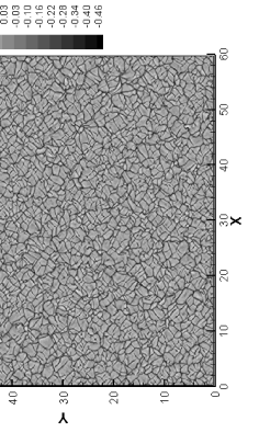
Figure 1.: Contours of the vertical component of velocity at depth 0 Mm .

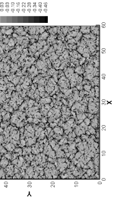
Figure 2.: Contours of the vertical component of velocity at depth 1 Mm.

Figure 3.: Contours of the vertical component of velocity at depth 2 Mm.

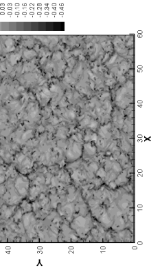
Figure 4.: Contours of the vertical component of velocity at depth 3 Mm.

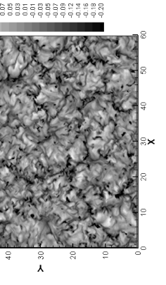
Figure 5.: Contours of the vertical component of velocity at depth 5 Mm.

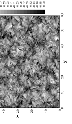
Figure 6.: Contours of the vertical component of velocity at depth 10 Mm.

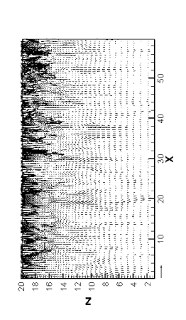
Figure 7.: The velocity field in a vertical plane.

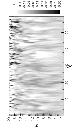
Figure 8.: Contours of vertical component of velocity field.

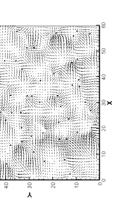
Figure 9.: The velocity field and location of corks.

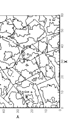
Figure 10.: Null contour of two-dimesional divergence of velocity and boundaries of supergranulation cells.

References

- Ustyugov (2006) Ustyugov, S. D., 2006, Numerical Modeling of Space Plasma Flows: Astronum-2006 ASP Conference Series, Volume 359, Proceedings of the Conference Held 26-30 March, 2006, in Palm Springs, California, USA. Edited by G. P. Zank and N. V. Pogorelov. San Francisco: Astronomical Society of the Pacific., p.226
- Stein & Nordlund (2006) Stein, R. F., & Nordlund, A., 2006, ApJ, 192, 91
- Christensen-Dalsgaard (2003) Christensen-Dalsgaard, J., 2003, Rev.Mod.Phys., 74, 1073
- Iglesias & Rogers (1996) Iglesias, C. A., & Rogers, F. J., 1996, ApJ, 464, 943
- Canuto et.al. (1994) Canuto, V. M., Minotti, F. O., & Schilling, J. L., 1994, ApJ, 425, 303
- Yee et.al. (1990) Yee, H. C., Kloppfer, G. H., & Montagne, J. L., 1990, JCP, 88, 31
- Shu & Osher (1988) Shu, C. W., & Osher, S., 1988, JCP, 77, 439