LSND versus MiniBooNE: Sterile neutrinos with energy dependent masses and mixing?

Abstract

Standard active–sterile neutrino oscillations do not provide a satisfactory description of the LSND evidence for neutrino oscillations together with the constraints from MiniBooNE and other null-result short-baseline oscillation experiments. However, if the mass or the mixing of the sterile neutrino depends in an exotic way on its energy all data become consistent. I explore the phenomenological consequences of the assumption that either the mass or the mixing scales with the neutrino energy as $1/E_{\nu}^{r}$ ($r>0$). Since the neutrino energy in LSND is about 40 MeV, whereas MiniBooNE operates at around 1 GeV, oscillations get suppressed in MiniBooNE and the two results become fully compatible for $r\gtrsim 0.2$. Furthermore, also the global fit of all relevant data improves significantly by exploring the different energy regimes of the various experiments. The best fit $\chi^{2}$ decreases by 12.7 (14.1) units with respect to standard sterile neutrino oscillations if the mass (mixing) scales with energy.

I Introduction

Reconciling the LSND evidence Aguilar:2001ty for $\bar{\nu}_{\mu}\to\bar{\nu}_{e}$ oscillations with the global neutrino data reporting evidence sk-atm ; lbl ; sno ; kamland and bounds karmen ; Astier:2003gs ; Dydak:1983zq ; Declais:1994su ; Apollonio:2002gd ; Boehm:2001ik on oscillations remains a long-standing problem for neutrino phenomenology. Recently the MiniBooNE experiment MB added more information to this problem. This experiment searches for $\nu_{\mu}\to\nu_{e}$ appearance with a very similar $L/E_{\nu}$ range as LSND. No evidence for oscillations is found and the results are inconsistent with a two-neutrino oscillation interpretation of LSND at 98% CL MB . The standard “solution” to the LSND problem is to introduce one or more sterile neutrinos at the eV scale sterile . However, it turns out that such sterile neutrino schemes do not provide a satisfactory description of all data in terms of neutrino oscillations, see Ref. Maltoni:2007zf for a recent analysis including MiniBooNE data; pre-MiniBooNE analyses can be found, e.g., in Refs. early ; strumia ; Maltoni:2002xd ; Sorel:2003hf ; Maltoni:2004ei . Apart from sterile neutrino oscillations, various more exotic explanations of the LSND signal have been proposed, for example, neutrino decay Ma:1999im ; Palomares-Ruiz:2005vf , CPT violation cpt ; strumia , violation of Lorentz symmetry lorentz , CPT-violating quantum decoherence Barenboim:2004wu , mass-varying neutrinos MaVaN , or shortcuts of sterile neutrinos in extra dimensions Pas:2005rb . See Refs. Strumia:2006db ; GonzalezGarcia:2007ib for two recent reviews.

In view of the difficulties to describe all data with “standard” sterile neutrino oscillations I assume in this note that the sterile neutrino is a more exotic particle than just a neutrino without weak interactions. Being a singlet under the Standard Model gauge group it seems possible that the sterile neutrino is a messenger from a hidden sector with some weired properties. I will assume in the following that the mass or the mixing of the fourth neutrino depends in a non-standard way on the neutrino energy. The motivation is that the neutrino energy in LSND is around 40 MeV, whereas MiniBooNE and the CDHS disappearance experiment operate around 1 GeV, and hence changing the energy dependence of oscillations will have some impact on the fit.

To be specific, I am going to assume that either the mass $m_{4}$ or the mixing $U_{\alpha 4}$ ($\alpha=e,\mu$) of the fourth neutrino state depends on the neutrino energy $E_{\nu}$ like

$$\text{MED:}\qquad\qquad m_{4}^{2}(E_{\nu}) =\tilde{m}_{4}^{2}\left(\frac{E_{\mathrm{ref}}}{E_{\nu}}\right)^{r}\,,$$ (1)

$$\text{EDM:}\qquad\quad|U_{\alpha 4}|^{2}(E_{\nu}) =|\tilde{U}_{\alpha 4}|^{2}\left(\frac{E_{\mathrm{ref}}}{E_{\nu}}\right)^{r}\,,$$

where $\tilde{m}_{4}$ and $\tilde{U}_{\alpha 4}$ are the mass and the mixing at a reference energy $E_{\mathrm{ref}}$, and for the exponent $r$ I will consider values in the interval $0\leq r\leq 1$. An energy dependent mass as in Eq. (1) will modify the energy dependence of oscillations from the standard $1/E_{\nu}$ dependence to $1/E_{\nu}^{1+r}$. Therefore, I refer to this effect as modified energy dependence (MED) oscillations, whereas the second case is denoted by energy dependent mixing (EDM). Most likely rather exotic physics will be necessary to obtain such a behaviour, some speculative remarks on possible origins are given in Sec. V. Here I make the assumptions of Eq. (1) without specifying any underlying model, instead I will explore the phenomenological consequences of MED and EDM oscillations for short-baseline neutrino data. I will show that in both cases (i) LSND and MiniBooNE become compatible and (ii) the global fit improves significantly.

It is important to note that Eq. (1) involves only the new fourth mass state, whereas masses and mixing of the three active Standard Model neutrinos are assumed to be constant. Therefore the successful and very robust description of solar, atmospheric, and long-baseline reactor and accelerator experiments sk-atm ; lbl ; sno ; kamland by three-flavour active neutrino oscillations is not altered significantly, since the mixing of the forth mass state with active neutrinos is small.

The outline of this paper is as follows. In Sec. II I discuss in some detail the framework of MED and EDM oscillations and give a qualitative discussion of the expected behaviour of the combined analysis of the relevant short-baseline oscillation data. In Sec. III the results of the numerical analysis are presented. The global fit includes the appearance experiments LSND, MiniBooNE, KARMEN and NOMAD, as well as various disappearance experiments. In Sec. IV I comment briefly on phenomenological consequences of MED/EDM oscillations in future oscillation experiments, astrophysics and cosmology. Sec. V presents some speculative thoughts on models leading to energy dependent masses and mixing for sterile neutrinos, and I summarize in Sec. VI.

II The MED and EDM oscillation frameworks

Before discussing qualitatively the phenomenological consequences of MED and EDM oscillations according to Eq. (1) let me briefly remind the reader about the description of short-baseline (SBL) neutrino oscillation data in the case of standard four-neutrino oscillations. In the so-called (3+1) schemes there is a hierarchy among the mass-squared differences:

$$\Delta m^{2}_{21}\ll|\Delta m^{2}_{31}|\ll\Delta m^{2}_{41}\,.$$ (2)

Under the assumption that $\Delta m^{2}_{21}$ and $\Delta m^{2}_{31}$ can be neglected SBL oscillations are described by two-flavour oscillation probabilities with an effective mixing angle depending on the elements of the lepton mixing matrix $|U_{e4}|^{2}$ and $|U_{\mu 4}|^{2}$. For $\nu_{\mu}\to\nu_{e}$ appearance experiments the effective mixing angle is given by

$$\sin^{2}2\theta_{\mu e}=4|U_{e4}|^{2}|U_{\mu 4}|^{2}\,,$$ (3)

whereas for a $\nu_{\alpha}$ disappearance experiment we have

$$\sin^{2}2\theta_{\alpha\alpha}=4|U_{\alpha 4}|^{2}(1-|U_{\alpha 4}|)^{2}\,,$$ (4)

see, e.g., Ref. Bilenky:1996rw . The fact that the amplitude responsible for the LSND appearance is a product of $|U_{e4}|^{2}$ and $|U_{\mu 4}|^{2}$, whereas $\nu_{e}$ and $\nu_{\mu}$ disappearance experiments constrain these elements separately leads to the well-known tension between LSND and disappearance experiments in the (3+1) oscillation schemes, see e.g., Refs. Bilenky:1996rw ; Okada:1996kw ; Barger:1998bn ; Bilenky:1999ny ; Peres:2000ic ; Grimus:2001mn ; cornering .

Assuming now an energy dependent mass for $\nu_{4}$ as in Eq. (1), it turns out that for the range of parameters and energies relevant for our discussion it is always possible to take $\nu_{4}$ much heavier than the three standard neutrinos, $m_{1,2,3}\ll m_{4}$, such that the usual SBL approximation Eq. (2) remains always valid, and the energy scaling of Eq. (1) applies also for the mass-squared difference $\Delta m^{2}_{41}(E_{\nu})\equiv m^{2}_{4}(E_{\nu})-m^{2}_{1}\approx m^{2}_{4}(E_{\nu})$. Then the relevant oscillation phase $\phi_{\mathrm{osc}}$ gets a different energy dependence than in the standard case:

$$\phi_{\mathrm{osc}}=\frac{\Delta m_{41}^{2}L}{4E_{\nu}}\approx\frac{\Delta\tilde{m}^{2}_{41}L}{4E_{\nu}}\left(\frac{E_{\mathrm{ref}}}{E_{\nu}}\right)^{r}\,.$$ (5)

Hence the standard $1/E_{\nu}$ dependence gets altered to $1/E_{\nu}^{1+r}$. The most relevant consequence of the MED with $r>0$ follows from Eq. (5): An experiment is sensitive to oscillations if $\phi_{\mathrm{osc}}\simeq\pi/2$, or

$$\frac{L}{E_{\nu}}\simeq\frac{2\pi}{\Delta\tilde{m}^{2}_{41}}\left(\frac{E_{\nu}}{E_{\mathrm{ref}}}\right)^{r}\,.$$ (6)

Hence, for experiments with $E_{\nu}>E_{\mathrm{ref}}$ the allowed region will be shifted to larger values of $\Delta\tilde{m}^{2}_{41}$ as compared to the standard oscillation case ($r=0$), whereas the allowed region for experiments with $E_{\nu}<E_{\mathrm{ref}}$ will be shifted to smaller $\Delta\tilde{m}^{2}_{41}$, in order to compensate for the factor $(E_{\nu}/E_{\mathrm{ref}})^{r}$ in Eq. (6).

Using instead of the MED now the energy dependence of the mixing matrix elements from Eq. (1), one obtains for the SBL appearance and disappearance amplitudes given in Eqs. (3) and (4):

$$\sin^{2}2\theta_{\mu e} =4|U_{e4}|^{2}|U_{\mu 4}|^{2}\propto\left(\frac{E_{\mathrm{ref}}}{E_{\nu}}\right)^{2r}\,,$$ (7)

$$\sin^{2}2\theta_{\alpha\alpha} =4|U_{\alpha 4}|^{2}(1-|U_{\alpha 4}|^{2})\approx 4|U_{\alpha 4}|^{2}\propto\left(\frac{E_{\mathrm{ref}}}{E_{\nu}}\right)^{r}\,.$$

This introduces only a mild distortion of the oscillation pattern from the standard oscillatory behaviour with $1/E_{\nu}$. The main effect of EDM is that the sensitivity of experiments with $E_{\nu}>E_{\mathrm{ref}}$ to the effective mixing angle gets weaker. Let us note that the EDM scaling of Eq. (1) cannot hold for arbitrarily low energies, simply because of unitarity of $U$. The low energy limit of the EDM scaling should find an explanation in some theory for this effect. Here I assume that for the parameter range relevant for the SBL analysis the power-law scaling of Eq. (1) remains valid.

Note that in both cases, MED and EDM, for fixed $r$ the choice of the reference energy $E_{\mathrm{ref}}$ is arbitrary. From Eq. (5) it is clear that choosing a different reference energy $E_{\mathrm{ref}}$ leads just to a rescaling of $\tilde{m}_{4}$ such that the combination $\Delta\tilde{m}^{2}_{41}E_{\mathrm{ref}}^{r}$ remains constant. Similar, changing $E_{\mathrm{ref}}$ in case of the EDM leads just to a rescaling of the $|\tilde{U}_{\alpha 4}|^{2}$. Hence, the (3+1) MED and EDM models have one phenomenological parameter in addition to the (3+1) standard oscillation model:

MED: $$|U_{e4}|^{2},\,|U_{\mu 4}|^{2},\,\Delta\tilde{m}^{2}_{41},\,r\,,$$ (8)

EDM: $$|\tilde{U}_{e4}|^{2},\,|\tilde{U}_{\mu 4}|^{2},\,\Delta m^{2}_{41},\,r\,.$$

The main effects of MED and EDM oscillations can be summarized in the following way: Consider the allowed regions of the various experiments for standard oscillations in the plane of $\sin^{2}2\theta_{\mu e}$ and $\Delta m^{2}_{41}$. Introducing now MED (EDM) leads to a relative shift of the regions of experiments at different energies along the $\Delta\tilde{m}^{2}_{41}$ ($\sin^{2}2\tilde{\theta}_{\mu e}$) axis. The relevant SBL experiments are listed in Tab. 1, ordered according to their mean neutrino energy. For convenience I will choose $E_{\mathrm{ref}}=40$ MeV, corresponding roughly to the mean neutrino energy in LSND. Since in MiniBooNE the neutrino energy is higher, for MED (EDM) oscillations the sensitivity is shifted to larger values of $\Delta\tilde{m}^{2}_{41}$ ($\sin^{2}2\tilde{\theta}_{\mu e}$) for $r>0$. In the MED framework MiniBooNE operates actually at a too small value of $L/E_{\nu}$ in order to test LSND. As I will show in the following, in both cases the two experiments become compatible for $r>0$. Furthermore, it turns out that also the global fit including all the experiments listed in the table improves significantly due to the different energy regimes.

Experiment	Ref.	Channel	Data	$\langle E_{\nu}\rangle$
Bugey	Declais:1994su	$\bar{\nu}_{e}\to\bar{\nu}_{e}$	60	4 MeV
Chooz	Apollonio:2002gd	$\bar{\nu}_{e}\to\bar{\nu}_{e}$	1	4 MeV
Palo Verde	Boehm:2001ik	$\bar{\nu}_{e}\to\bar{\nu}_{e}$	1	4 MeV
LSND	Aguilar:2001ty	$\bar{\nu}_{\mu}\to\bar{\nu}_{e}$	11	40 MeV
KARMEN	karmen	$\bar{\nu}_{\mu}\to\bar{\nu}_{e}$	9	40 MeV
MiniBooNE	MB	$\nu_{\mu}\to\nu_{e}$	8	700 MeV
CDHS	Dydak:1983zq	$\nu_{\mu}\to\nu_{\mu}$	15	1 GeV
NOMAD	Astier:2003gs	$\nu_{\mu}\to\nu_{e}$	1	50 GeV

Table 1: Experiments used in the SBL analysis. The oscillation channel, and the number of data points used in the fit (“Data”) are given. The last column shows the approximate mean neutrino energy for each experiment.

III Global analysis of SBL data for MED and EDM oscillations

III.1 Description of the data used in the fit

Before presenting the results of the analysis let us briefly discuss the data used in the fit, as summarized in Tab. 1. For the re-analysis of LSND I fit the observed transition probability (total rate) plus 11 data points of the $L/E$ spectrum with free normalisation, both derived from the decay-at-rest data Aguilar:2001ty . For KARMEN the data observed in 9 bins of prompt energy as well as the expected background karmen is used in the fit. Further details of the LSND and KARMEN analyses are given in Ref. Palomares-Ruiz:2005vf . For NOMAD I fit the total rate using the information provided in Ref. Astier:2003gs .

The MiniBooNE analysis is based on the information provided at the web-page MB-data , derived from the actual Monte Carlo simulation performed by the collaboration. Using these data the “official” MiniBooNE analysis MB can be reproduced with very good accuracy. The averaging of the transition probability is performed with the proper reconstruction efficiencies, and detailed information on error correlations and backgrounds is available for the $\chi^{2}$ analysis. MiniBooNE data are consistent with zero (no excess) above 475 MeV, whereas below this energy a $3.6\sigma$ excess of $96\pm 17\pm 20$ events is observed. Whether this excess comes indeed from $\nu_{\mu}\to\nu_{e}$ transitions or has some other origin is under investigation. As discussed in Ref. MB , standard two-neutrino oscillations cannot account for the event excess at low energies. Following the strategy of the MiniBooNE collaboration the analysis is restricted to the energy range from 475 MeV to 3 GeV. In Sec. III.3 I will comment on the possibility to obtain the low energy event excess in case of MED oscillations.

I include the disappearance experiments Bugey Declais:1994su , Chooz Apollonio:2002gd , and Palo Verde Boehm:2001ik (reactor $\bar{\nu}_{e}$ disappearance), as well as the CDHS Dydak:1983zq $\nu_{\mu}$ disappearance experiment, see Ref. Grimus:2001mn for technical details. In addition to the data listed in Tab. 1 atmospheric neutrino data give an important constraint on the mixing of $\nu_{\mu}$ with the heavy mass state, i.e., on $|U_{\mu 4}|^{2}$ Bilenky:1999ny ; cornering . I use the updated analysis described in detail in Ref. Maltoni:2007zf . The basic assumption in this analysis is that $\Delta m^{2}_{41}$ is “infinite” for atmospheric neutrinos according to Eq. (2). Since I assume this to be true also in the scenarios under consideration one can directly apply the bound on $|U_{\mu 4}|^{2}$ from the standard oscillation analysis. In case of EDM one should perform a re-analysis of atmospheric data taking into account the energy dependence of $|U_{\mu 4}|^{2}$ for the various data samples spanning five decades in neutrino energy. Such an analysis is beyond the scope of the present work and I assume a scaling of $|U_{\mu 4}|^{2}$ corresponding to an average energy of 1 GeV. Adding one data point for the bound from atmospheric neutrinos to the data given in Tab. 1 I obtain $N_{\mathrm{tot}}=107$ data points in the global analysis.

III.2 Results of the global analysis

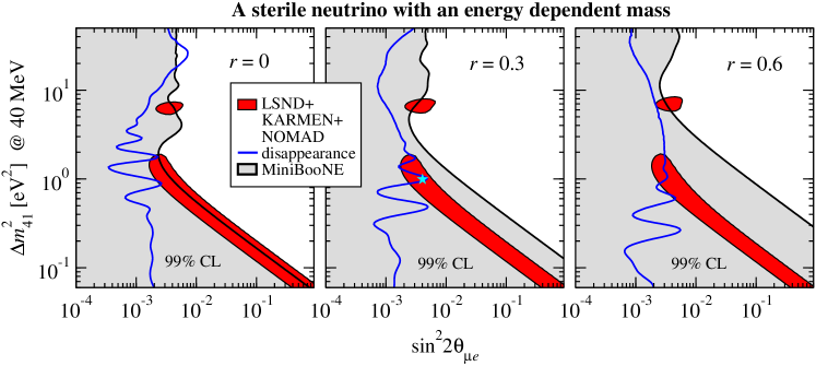
Figure 1: (3+1) oscillations with a modified energy dependence (MED): Allowed regions at 99% CL (2 d.o.f.) for LSND+KARMEN+NOMAD, MiniBooNE, and the disappearance experiments for standard oscillations $r=0$ (left) and MED oscillations with $r=0.3$ (middle) and $r=0.6$ (right). The star in the middle panel corresponds to the global best fit point.

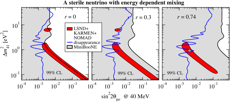
Figure 2: (3+1) oscillations with energy dependent mixing (EDM): Allowed regions at 99% CL (2 d.o.f.) for LSND+KARMEN+NOMAD, MiniBooNE, and the disappearance experiments for standard oscillations $r=0$ (left) and EDM oscillations with $r=0.3$ (middle) and $r=0.74$ (right). The star in the right panel corresponds to the global best fit point.

Let us now discuss the results of the numerical analysis within the frameworks of MED and EDM oscillations. Figs. 1 and 2 show the allowed regions in the plane of $\Delta m^{2}_{41}$ and $\sin^{2}2\theta_{\mu e}$ for various data sets for standard oscillations ($r=0$) compared to the exotic energy dependence models for some values of $r>0$. First, note that the neutrino energy in LSND and KARMEN is the same, and therefore the consistency of LSND and KARMEN Church:2002tc is not affected by introducing a non-zero $r$. Furthermore, since we choose a reference energy $E_{\mathrm{ref}}$ close to the mean energy in these experiments the allowed region from LSND+KARMEN+NOMAD does not change by increasing $r$. Second, in agreement with the argument given in Sec. II one observes from the figures that the bound from MiniBooNE moves to higher values of $\Delta m^{2}_{41}$ for MED and to higher values of $\sin^{2}2\theta_{\mu e}$ for EDM if $r$ increases, as a consequence of the higher neutrino energy in MiniBooNE. I find that in both cases for $r\gtrsim 0.2$ LSND and MiniBooNE are fully consistent. Third, Figs. 1 and 2 show the bound on $\sin^{2}2\theta_{\mu e}$ from the disappearance experiments Bugey, Chooz, Palo Verde, CDHS, and atmospheric neutrino data, where for a given $\sin^{2}2\theta_{\mu e}$ I minimize the $\chi^{2}$ with respect to $|U_{e4}|^{2}$ and $|U_{\mu 4}|^{2}$ under the constraint $\sin^{2}2\theta_{\mu e}=4|U_{e4}|^{2}|U_{\mu 4}|^{2}$. As visible in the left panels, in the standard oscillation case there is severe tension between these data and the LSND evidence, and at 99% CL there is basically no overlap of the allowed regions. However, the situation clearly improves for MED and EDM oscillations, and for $r>0$ the allowed regions overlap.

For MED oscillations (Fig. 1) this can be understood in the following way. The pronounced wiggles in the disappearance bound visible in the left panel around $\Delta m^{2}_{41}\sim 1$ eV² come from the Bugey reactor experiment. Since $E_{\nu}$ for Bugey is smaller than the reference energy of 40 MeV these features move to lower values of $\Delta\tilde{m}^{2}_{41}$ if $r$ is increased. On the other hand, the constraint on $|U_{\mu 4}|^{2}$ from CDHS is shifted to higher values of $\Delta\tilde{m}^{2}_{41}$ and only the weaker constraint from atmospheric data remains. Both trends work together in moving the disappearance bound towards the LSND region, as visible in the middle panel for $r=0.3$. If $r$ is further increased the Bugey pattern moves to even smaller values of $\Delta\tilde{m}^{2}_{41}$, and the bound at the relevant region around 1 eV² is given by the constraints from Chooz on $|U_{e4}|^{2}$ and atmospheric neutrinos on $|U_{\mu 4}|^{2}$ (see right panel).

In the case of EDM oscillations (Fig. 2) there are two opposite trends. Since for Bugey $E_{\nu}<E_{\mathrm{ref}}$ the constraint on $|\tilde{U}_{e4}|^{2}$ becomes stronger with increasing $r$, whereas for CDHS and atmospheric data $E_{\nu}>E_{\mathrm{ref}}$ and the bound on $|\tilde{U}_{\mu 4}|^{2}$ gets weaker. The upper limit on $\sin^{2}2\tilde{\theta}_{\mu e}$ emerges from the product of these two constraints, see Eq. (3), and therefore, it scales according to

$$\left(\frac{E_{\mathrm{ref}}^{2}}{\langle E_{\nu}\rangle_{\mathrm{Bugey}}\,\langle E_{\nu}\rangle_{\mathrm{CDHS,atm}}}\right)^{r}\simeq 0.4^{r}\,.$$ (9)

Hence, the net-effect is a shift of the bound to larger values of $\sin^{2}2\tilde{\theta}_{\mu e}$ and a significant overlap with the LSND region emerges.

Fig. 3 shows the $\chi^{2}$ for appearance data only (left) and for the global data (right) as a function of the energy exponent $r$. The best fit points have the following $\chi^{2}$ values:

MED: $$\chi^{2}_{\mathrm{app,min}}=19.4/(29-3)\,\text{d.o.f.}\,,\qquad\chi^{2}_{\mathrm{glob,min}}=89.0/(107-4)\,\text{d.o.f.}\,,$$ (10)

EDM: $$\chi^{2}_{\mathrm{app,min}}=19.6/(29-3)\,\text{d.o.f.}\,,\qquad\chi^{2}_{\mathrm{glob,min}}=87.6/(107-4)\,\text{d.o.f.}\,,$$

and occur at the parameter values

MED: $$|U_{e4}|=0.15,\,|U_{\mu 4}|=0.21,\,\Delta\tilde{m}^{2}_{41}=1.0~{}\text{eV}^{2},\,r=0.3\,,$$ (11)

EDM: $$|\tilde{U}_{e4}|=0.06,\,|\tilde{U}_{\mu 4}|=0.53,\,\Delta m^{2}_{41}=0.92~{}\text{eV}^{2},\,r=0.74\,.$$

As mentioned above, the parameters with tilde correspond always to a reference energy of 40 MeV. In agreement with the discussion above one observes that for EDM $|\tilde{U}_{e4}|$ is rather small to respect the stronger bound from Bugey, whereas $|\tilde{U}_{\mu 4}|$ gets relatively large due to the relaxed bound from CDHS and atmospheric data. Although the best fit point for EDM occurs at the relatively large value of $r=0.74$, one can see from Fig. 3 that fits of comparable quality are obtained already for $r\gtrsim 0.4$.

The MED and EDM fits improves significantly with respect to the standard oscillation case $r=0$:

MED: $$\Delta\chi^{2}_{\mathrm{app}}(r=0)=7.7\,,\qquad\Delta\chi^{2}_{\mathrm{glob}}(r=0)=12.7\,,$$ (12)

EDM: $$\Delta\chi^{2}_{\mathrm{app}}(r=0)=7.5\,,\qquad\Delta\chi^{2}_{\mathrm{glob}}(r=0)=14.1\,.$$

For comparison, the extension of the standard (3+1) oscillation scheme to a (3+2) scheme by the addition of a second sterile neutrino leads to an improvement of $\chi^{2}_{\mathrm{min\,(3+1)}}-\chi^{2}_{\mathrm{min\,(3+2)}}=6.1$ Maltoni:2007zf . Taking into account that for (3+2) oscillations 4 additional parameters are introduced in the fit instead of only one as in the cases of MED or EDM, one concludes that the latter provide a much more significant improvement of the fit.

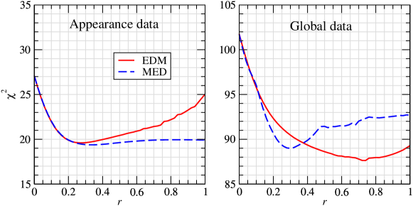
Figure 3: The $\chi^{2}$ for SBL appearance data (left) and global data (right) for MED and EDM oscillations as a function of the exponent $r$, minimized with respect to the other parameters. The number of data points is 29 for the appearance experiments and 107 for the global analysis.

The shape of the curves in Fig. 3 can be understood from the behaviour of the allowed regions shown in Figs. 1 and 2. The best fit for appearance data is reached once the MiniBooNE exclusion curve is moved out of the LSND region, and no further improvement can be obtained by further increasing $r$. In the case of EDM the fit gets worse again due to the energy distortion introduced for large $r$ by scaling the mixing with $1/E_{\nu}^{r}$. This is also the reason for the change in the LSND region visible in the right panel of Fig. 2. For MED, the global $\chi^{2}$ reaches a minimum when the wiggles from the Bugey bound cover the LSND region around $\Delta\tilde{m}^{2}_{41}\simeq 1~{}\text{eV}^{2}$. If $r$ is further increased these wiggles are moved out again of the LSND region and the fit gets slightly worse again. For $r\gtrsim 0.5$ a plateau is reached, since then the disappearance bound at $\Delta\tilde{m}_{41}\simeq 1~{}\text{eV}^{2}$ comes mainly from Chooz and atmospheric data, which are independent of $\Delta m^{2}_{41}$ and hence also independent of $r$. In the case of EDM, the global $\chi^{2}$ improves until relatively large values of $r$ as a consequence of Eq. (9). At some point again the fit gets worse due to the anomalous energy dependence of the probability.

A powerful tool to evaluate the compatibility of different data sets is the so-called parameter goodness-of-fit (PG) criterion discussed in Ref. Maltoni:2003cu . It is based on the $\chi^{2}$ function

$$\chi^{2}_{\text{PG}}=\chi^{2}_{\text{tot,min}}-\sum_{i}\chi^{2}_{i,\text{min}}\,,$$ (13)

where $\chi^{2}_{\text{tot,min}}$ is the $\chi^{2}$ minimum of all data sets combined and $\chi^{2}_{i,\text{min}}$ is the minimum of the data set $i$. This $\chi^{2}$ function measures the “price” one has to pay by the combination of the data sets compared to fitting them independently. It should be evaluated for the number of d.o.f. corresponding to the number of parameters in common to the data sets, see Ref. Maltoni:2003cu for a precise definition.

	Standard oscillations		MED oscillations		EDM oscillations
Data sets	$\chi^{2}_{\mathrm{PG}}/$d.o.f.	PG	$\chi^{2}_{\mathrm{PG}}/$d.o.f.	PG	$\chi^{2}_{\mathrm{PG}}/$d.o.f.	PG
LSND vs NEV	24.9/2	$4\times 10^{-6}$	14.0/3	$0.3\%$	11.9/3	$0.8\%$
LSND vs NEV-APP vs DIS	25.3/4	$4\times 10^{-5}$	14.3/6	$3\%$	12.3/6	$5\%$
LKN vs MiniBooNE vs DIS	20.1/4	$5\times 10^{-5}$	8.9/6	$18\%$	6.7/6	$35\%$

Table 2: Consistency tests of various data sub-sets for standard (3+1) oscillations, MED and EDM oscillations. The data sets are SBL data showing no evidence for oscillations (NEV), no-evidence appearance data (NEV-APP = MiniBooNE + KARMEN + NOMAD), SBL disappearance data (DIS), and LSND + KARMEN + NOMAD (LKN). I give $\chi^{2}_{\mathrm{PG}}$ according to Eq. (13) and the corresponding probability (“PG”).

The results of such a PG analysis are displayed in Tab. 2. First, the compatibility of LSND and all the remaining no-evidence SBL data is tested, and the PG is compared within the standard, the MED, and the EDM oscillation frameworks. The consistency improves drastically from $4\times 10^{-6}$ to $3\times 10^{-3}$ (MED) or $8\times 10^{-3}$ (EDM). The probability value in the MED case corresponds to a tension of slightly less than $3\sigma$. Second, as an alternative test I check the compatibility of the three data sets LSND, no-evidence appearance data, and disappearance data. Similar a huge improvement of the consistency from $4\times 10^{-5}$ for standard oscillations to 3% (MED) or 5% (EDM) is found.

Although both of these two tests clearly show an improvement of the fit with respect to standard oscillations, the low probabilities still indicate that the global fit is not perfect and some tension remains in the data. The reason for this is the tension between KARMEN and LSND, which is the same as in the standard oscillation case, since these experiments have the same energy. The allowed regions in the space of oscillation parameters of these two experiments have clearly an overlap, and a careful combined analysis came to the conclusion that they are consistent Church:2002tc . Nevertheless, there remains a tension between them which is detected by the rather sensitive PG test. In the last row of Tab. 2 I consider the case when LSND and KARMEN are combined to one single data set (which includes also NOMAD), and test the consistency of this set against MiniBooNE and disappearance data. This corresponds to the data sets shown in Figs. 1 and 2, and since LSND and KARMEN are included in the same data set the tension between them does not show up in the PG. In this case the PG shows a perfect consistency of all data with probablities of 18% and 35% for MED and EDM, respectively, whereas the probablitiy of standard oscillations remains unacceptably low.

III.3 The low energy excess in MiniBooNE

Before concluding this section I comment briefly on the event excess observed in MiniBooNE in the energy region below 475 MeV. As discussed in Ref. MB , standard two-flavour oscillations cannot account for the sharp rise at low energy. However, since in the MED scenario the energy dependence of oscillations is modified according to Eq. (5) one may expect that an explanation of the excess becomes possible. Indeed I find that for values of the exponent $r\gtrsim 1$ the rise of the oscillation probability becomes steep enough and a perfect fit to the full spectrum including the excess between 300 and 475 MeV becomes possible. For such large values of $r$ a closed allowed region appears in the plane of $\Delta\tilde{m}^{2}_{41}$ and $\sin^{2}2\theta_{\mu e}$ for MiniBooNE data (not only a bound). However, because of the large $r$ value this allowed region appears at $\Delta\tilde{m}^{2}_{41}$ values above the LSND region and the KARMEN bound. Hence, although a modified energy dependence like considered here allows in principle for an explanation of the low energy event excess, this solution is not compatible with LSND and the KARMEN bound, and in the global analysis the excess cannot be fitted. For this reason I used in the analysis only the MiniBooNE data above 475 MeV MB , and rely on an alternative explanation of the low energy event excess.

IV Implications for future experiments, astrophysics and cosmology

In this section I briefely comment on other phenomenological implications of the MED/EDM schemes. In general the scenarios considered here are difficult to test at future neutrino oscillation experiments. No appearance signal is expected for MiniBooNE anti-neutrino data, which currently are being accumulated, since the energy dependence is assumed to affect anti-neutrinos in the same way as neutrinos. In order to test the LSND signal for a MED with $r=0.3$ at the given MiniBooNE baseline one would need to run at an energy of

$$E_{\mathrm{MiniBooNE}}^{\mathrm{MED}}\simeq\left(\frac{L_{\mathrm{MiniBooNE}}}{L_{\mathrm{LSND}}}\right)^{\frac{1}{1+r}}E_{\mathrm{LSND}}\approx\left(\frac{540\,\mathrm{m}}{30\,\mathrm{m}}\right)^{0.77}40\,\mathrm{MeV}\approx 360\,\mathrm{MeV}\,,$$ (14)

which seems not practicable because of low cross sections and large backgrounds. A similar signal as in standard (3+1) or (3+2) oscillations is expected also in the MED scenario for future reactor experiments, see Ref. Bandyopadhyay:2007rj . A promising place to look for effects of MED oscillations could be the 2 km detector proposed for the T2K experiment Itow:2001ee . With a mean neutrino energy of 0.7 GeV this detector is slightly too far from the neutrino source to cover the oscillation maximum in case of standard oscillations with $\Delta m^{2}\sim 1$ eV². However, with the MED best fit point from Eq. (11) the oscillation phase according to Eq. (5) turns out to be close to $\pi/2$ at $L=2$ km.

A rather model independent test of MED or EDM explanations of LSND would be an experiment operating at the same energy as LSND, such as proposed in Ref. Garvey:2005pn . Furthermore, to test the EDM scenario one would like to perform experiments at energies as small as possible. In particular, this model predicts relatively large effects for $\nu_{\mu}$ disappearance for experiments at energies smaller than 1 GeV, since the eV-scale mass state has a rather large mixing with $\nu_{\mu}$ at 40 MeV, see Eq. (11). Let us note that unitarity requires $|U_{\alpha 4}|\leq 1$. Therefore, the power law energy dependence of EDM cannot hold down to arbitrarily low energies. At the best fit values given in Eq. (11), one finds $|U_{e4}|\simeq 1$ at $E_{\nu}\simeq 0.02$ MeV and $|U_{\mu 4}|\simeq 1$ at $E_{\nu}\simeq 7$ MeV. In order to use the EDM framework for very low energies one would have to specify the energy dependence of the neutrino mass matrix, and obtain the mixing angles via the diagonalisation, such that unitarity is always guaranteed. This is especially relevant, for example, to obtain predictions for neutrino mass experiments from Tritium beta-decay, which has an end point energy of 18.6 keV.

As in case of standard sterile neutrino mixing, also in the MED/EDM framework the sterile neutrinos have implications for cosmology and astrophysics, see Ref. Cirelli:2004cz and references therein. In general the effects will be very similar to the standard case with effective masses and mixing evaluated according to the relevant neutrino energy. For example, in a supernova and in Big Bang nucleosynethesis (BBN) the neutrino energy is close to (or slightly below) the reference energy 40 MeV used above, and therefore the mixing parameters shown in Eq. (11) roughly apply in these environments. This implies that—as in the standard (3+1) case—the sterile neutrino will be brought into thermal equilibrium via oscillations prior to BBN Okada:1996kw ; DiBari:2003fg .

Cosmology provides a bound on the sum of the neutrino masses in the sub-eV range cosmo-bounds , mainly from the power spectrum at large scales combined with precise data on the cosmic microwave background. In general this bound implies a challenge for sterile neutrino schemes relevant for LSND. The conflict becomes particularly severe for the MED framework, since here the neutrino mass increases with decreasing neutrino energy, which implies large masses for cosmological relevant neutrinos. Let us note, however, that depending on the particular model realisation of MED one can expect that the power law scaling of Eq. (1) does not continue down to arbitrarily low energies. Here I assume only that it holds in the energy interval relevant for SBL experiments, i.e., above about 1 MeV, and it might be altered at lower energies.

V Speculations on model realisations of MED/EDM

Before concluding I give here some speculative thoughts on possible reasons for a power law scaling of sterile neutrino masses or mixing. Without doing any detailed model building I just mention a few possibilities where such a behaviour might occur.

Indeed, energy dependent neutrino masses and mixing are a very familiar phenomenon in the framework of the standard matter effect MSW . Since the effective matter potential depends on the neutrino energy the mass eigenstates and mixing angles in matter depend on the energy. An analogous mechanism would be at work for the sterile neutrino if it interacts with some un-known background field or has some special interactions with standard matter. Such a possibility has been noted in Ref. Strumia:2006db and explored recently in Ref. Nelson:2007yq . The interaction postulated for the sterile neutrino should be several orders of magnitude stronger than usual weak interactions in order to be relevant at the short baselines in LSND or MiniBooNE. In these models neutrinos and anti-neutrinos interact differently and therefore they will have a different energy dependence. This may change the null-prediction for the MiniBooNE search with anti-neutrinos mentioned in the previous section.

An energy dependence similar to a matter potential occurs also in the model of Ref. Pas:2005rb , where sterile neutrinos are allowed to take shortcuts through particularly shaped extra dimensions. Effectively this leads to a modification of the dispersion relation of the sterile neutrinos which introduces a non-standard energy dependence on active–sterile oscillations. In general also a violation of the Lorentz symmetry such as considered for example in Ref. lorentz leads to oscillations with an energy dependence different from the standard one.

Another motivation for energy dependent neutrino masses and/or mixing could be the idea of “unparticle” physics Georgi:2007ek . One assumes the existence of a scale invariant sector with a non-trivial infrared fixed point coupled to the Standard Model through non-renormalizable operators. Such operators may have large anomalous dimensions and hence introduce power-law running of coupling constants. For example, suppose a fermionic unparticle operator ${\mathcal{O}}_{N}$ with mass-dimension $d_{N}$, with $3/2<d_{N}<5/2$, which has the quantum numbers of a right-handed neutrino (and hence is a gauge singlet). Then one can write a “mass term” $m_{\alpha}\overline{\nu}_{\alpha}{\mathcal{O}}_{N}$, where $\nu_{\alpha}$ can be either an active left-handed neutrino, or a “standard” sterile neutrino. The dimension of $m_{\alpha}$ is $5/2-d_{N}$ with the anomalous dimension $3/2-d_{N}$. Assuming that the coupling of ${\mathcal{O}}_{N}$ with $\nu_{\alpha}$ is scale invariant implies that the effective “masses” at two energy scales $\Lambda_{1}$ and $\Lambda_{2}$ are related by $m_{\alpha}(\Lambda_{1})=(\Lambda_{2}/\Lambda_{1})^{d_{N}-3/2}m_{\alpha}(\Lambda_{2})$. This resembles the scaling of Eq. (1), relating the phenomenological parameter $r$ in the above analysis to the anomalous dimension of the unparticle operator. The physical neutrino masses have to be found as poles in the corresponding propagator. These arguments provide a hint that the unparticle framework might lead to the exoting energy dependence of Eq. (1); whether it is indeed possible to obtain a valid model for MED and/or EDM active–sterile neutrino oscillations using unparticles needs further investigation, which is beyond the scope of this work.

Via the so-called AdS/CFT correspondence effects from a conformal sector such as mentioned above might actually have an interpretation also in theories with extra spacetime dimensions. In such models couplings can exhibit power law running Dienes:1998vh . If the neutrino mass is generated through a mechanism involving extra dimensions Dienes:1998sb their masses and mixing may depend on energy through these running effects. Usually the scale of new physics in extra dimensional models is around or above the TeV energy scale. In order to be relevant for the LSND/MiniBooNE problem one has to assume that the mechanism responsible for the power law running can be extended to the energy scale relevant for the experiments under consideration (MeV to GeV) in the active–sterile neutrino sector.

At this point I will not go into further details and leave the question whether indeed a full model for MED or EDM oscillations can be constructed from any of the mentioned mechanisms open for future work. I add that in a given realisation the energy dependence might be different than assumed in Eq. (1). However, the generic assumption of a power law should be a reasonable approximation in many cases and capture the relevant phenomenology.

VI Conclusions

I have considered short-baseline (SBL) neutrino oscillation data including LSND and MiniBooNE in the framework of sterile neutrino oscillations, assuming that the properties of the sterile neutrino depend on its energy in a rather exotic way. Along these lines I considered two different scenarios. First, I have assumed that the mass of the sterile neutrino scales with its energy as $1/E_{\nu}^{r}$ ($0\leq r\leq 1$). This introduces a modified energy dependence (MED) in oscillations: Instead of the standard $1/E_{\nu}$ dependence one obtains a MED with $1/E_{\nu}^{1+r}$. Second, I have assumed an energy dependent mixing (EDM) of the sterile neutrino with the active ones, namely that the elements of the mixing matrix $|U_{e4}|^{2}$ and $|U_{\mu 4}|^{2}$ scale with $1/E_{\nu}^{r}$. In a given model realisation one can expect that both, masses as well as mixing depend on energy in a correlated way. Here I have not specified any underlying theory, and a phenomenological analysis has been performed assuming the presence of either MED or EDM separately, to show the impact on the global fit of SBL data. For a given model it is easy to generalise the analysis and estimate the effect of the simultaneous scaling of masses and mixing.

I find that under the hypothesis of MED or EDM oscillations LSND and MiniBooNE data become fully consistent, and the bound from disappearance data overlaps with the LSND allowed region. The global fit including all relevant appearance and disappearance experiments improves by 12.7 (MED) or 14.1 (EDM) units in $\chi^{2}$ with respect to the standard (3+1) oscillation case, and the consistency of LSND with no-evidence appearance experiments and with disappearance experiments improves from $4\times 10^{-5}$ for standard oscillations to 3% (MED) or 5% (EDM). If the tension between LSND and KARMEN is removed from the analysis perfect consistency of all data is found, with probablities of 18% and 35% for MED and EDM, respectively, whereas the probablitiy of standard oscillations remains unacceptably low. Consistency of the global data is obtained in the MED framework by shifting the sensitivity of high energy experiments like MiniBooNE and CDHS to larger values of $L/E_{\nu}$ with respect to low energy experiments like LSND and Bugey. In the case of EDM oscillations the sensitivity of high energy experiments to the mixing angle gets weaker compared to low energy experiments, leading to consistency of all data.

In summary, I have shown that under the assumption of a non-standard energy dependence of sterile neutrino oscillations the description of global SBL data is significantly improved. This result is based on the fact that various experiments operate at different energy regimes.

Acknowledgment. I would like to thank Sacha Davidson for initiating this analysis, and for lots of discussions. Furthermore, I thank Giacomo Cacciapaglia, Roberto Contino, Alan Cornell, Naveen Gaur, Jörn Kersten, and Riccardo Rattazzi for discussions on the possibility to obtain MED and/or EDM like in Eq. (1) using the concept of un-particle physics.

References

- (1) A. Aguilar et al. [LSND Coll.], “Evidence for neutrino oscillations from the observation of appearance in a beam,” Phys. Rev. D 64, 112007 (2001) [hep-ex/0104049].
- (2) Y. Fukuda et al. [Super-Kamiokande Coll.], “Evidence for oscillation of atmospheric neutrinos,” Phys. Rev. Lett. 81, 1562 (1998) [hep-ex/9807003]; Y. Ashie et al., “A measurement of atmospheric neutrino oscillation parameters by Super-Kamiokande I,” Phys. Rev. D 71, 112005 (2005) [hep-ex/0501064].
- (3) E. Aliu et al. [K2K Coll.], “Evidence for muon neutrino oscillation in an accelerator-based experiment,” Phys. Rev. Lett. 94, 081802 (2005) [hep-ex/0411038]; D. G. Michael et al. [MINOS Coll.], “Observation of muon neutrino disappearance with the MINOS detectors and the NuMI neutrino beam,” Phys. Rev. Lett. 97, 191801 (2006) [hep-ex/0607088].
- (4) Q. R. Ahmad et al. [SNO Coll.], “Direct evidence for neutrino flavor transformation from neutral-current interactions in the Sudbury Neutrino Observatory,” Phys. Rev. Lett. 89, 011301 (2002) [nucl-ex/0204008].
- (5) T. Araki et al., “Measurement of neutrino oscillation with KamLAND: Evidence of spectral distortion,” Phys. Rev. Lett. 94, 081801 (2005) [hep-ex/0406035].
- (6) B. Armbruster et al. [KARMEN Coll.], “Upper limits for neutrino oscillations from muon decay at rest,” Phys. Rev. D 65, 112001 (2002) [hep-ex/0203021].
- (7) P. Astier et al. [NOMAD Coll.], “Search for oscillations in the NOMAD experiment,” Phys. Lett. B 570, 19 (2003) [hep-ex/0306037].
- (8) F. Dydak et al., “A Search For Muon-Neutrino Oscillations In The Range To ,” Phys. Lett. B 134, 281 (1984).
- (9) Y. Declais et al., “Search for neutrino oscillations at 15-meters, 40-meters, and 95-meters from a nuclear power reactor at Bugey,” Nucl. Phys. B 434, 503 (1995).
- (10) M. Apollonio et al., “Search for neutrino oscillations on a long base-line at the CHOOZ nuclear power station,” Eur. Phys. J. C 27, 331 (2003) [hep-ex/0301017].
- (11) F. Boehm et al., “Final results from the Palo Verde neutrino oscillation experiment,” Phys. Rev. D 64, 112001 (2001) [hep-ex/0107009].
- (12) A. A. Aguilar-Arevalo et al. [MiniBooNE Coll.], “A Search for Electron Neutrino Appearance at the Scale,” Phys. Rev. Lett. 98, 231801 (2007) [arXiv:0704.1500].
- (13) J. T. Peltoniemi, D. Tommasini and J. W. F. Valle, “Reconciling dark matter and solar neutrinos,” Phys. Lett. B 298, 383 (1993); J. T. Peltoniemi and J. W. F. Valle, “Reconciling dark matter, solar and atmospheric neutrinos,” Nucl. Phys. B 406, 409 (1993) [hep-ph/9302316]; D.O. Caldwell and R.N. Mohapatra, “Neutrino mass explanations of solar and atmospheric neutrino deficits and hot dark matter,” Phys. Rev. D 48, 3259 (1993).
- (14) M. Maltoni and T. Schwetz, “Sterile neutrino oscillations after first MiniBooNE results,” Phys. Rev. D 76 (2007) 093005 [arXiv:0705.0107].
- (15) J. J. Gomez-Cadenas and M. C. Gonzalez-Garcia, “Future Tau-Neutrino Oscillation Experiments And Present Data,” Z. Phys. C 71, 443 (1996) [hep-ph/9504246]; S. Goswami, “Accelerator, reactor, solar and atmospheric neutrino oscillation: Beyond three generations,” Phys. Rev. D 55, 2931 (1997) [hep-ph/9507212].
- (16) A. Strumia, “Interpreting the LSND anomaly: Sterile neutrinos or CPT-violation or…?,” Phys. Lett. B 539, 91 (2002) [hep-ph/0201134].
- (17) M. Maltoni, T. Schwetz, M. A. Tortola and J. W. F. Valle, “Ruling out four-neutrino oscillation interpretations of the LSND anomaly?,” Nucl. Phys. B 643, 321 (2002) [hep-ph/0207157].
- (18) M. Sorel, J. M. Conrad and M. Shaevitz, “A combined analysis of short-baseline neutrino experiments in the (3+1) and (3+2) sterile neutrino oscillation hypotheses,” Phys. Rev. D 70, 073004 (2004) [hep-ph/0305255].
- (19) M. Maltoni, T. Schwetz, M. A. Tortola and J. W. F. Valle, “Status of global fits to neutrino oscillations,” New J. Phys. 6, 122 (2004) [hep-ph/0405172 v5].
- (20) E. Ma, G. Rajasekaran and I. Stancu, “Hierarchical four-neutrino oscillations with a decay option,” Phys. Rev. D 61, 071302 (2000) [hep-ph/9908489]; E. Ma and G. Rajasekaran, “Light unstable sterile neutrino,” Phys. Rev. D 64, 117303 (2001) [hep-ph/0107203].
- (21) S. Palomares-Ruiz, S. Pascoli and T. Schwetz, “Explaining LSND by a decaying sterile neutrino,” JHEP 0509, 048 (2005) [hep-ph/0505216].
- (22) H. Murayama and T. Yanagida, “LSND, SN1987A, and CPT violation,” Phys. Lett. B 520, 263 (2001) [hep-ph/0010178]; G. Barenboim, L. Borissov and J. Lykken, “CPT violating neutrinos in the light of KamLAND,” hep-ph/0212116; M. C. Gonzalez-Garcia, M. Maltoni and T. Schwetz, “Status of the CPT violating interpretations of the LSND signal,” Phys. Rev. D 68, 053007 (2003) [hep-ph/0306226]; V. Barger, D. Marfatia and K. Whisnant, “LSND anomaly from CPT violation in four-neutrino models,” Phys. Lett. B 576, 303 (2003) [hep-ph/0308299].
- (23) V. A. Kostelecky and M. Mewes, “Lorentz violation and short-baseline neutrino experiments,” Phys. Rev. D 70, 076002 (2004) [hep-ph/0406255]; A. de Gouvea and Y. Grossman, “A three-flavor, Lorentz-violating solution to the LSND anomaly,” Phys. Rev. D 74, 093008 (2006) [hep-ph/0602237]; T. Katori, A. Kostelecky and R. Tayloe, “Global three-parameter model for neutrino oscillations using Lorentz violation,” Phys. Rev. D 74, 105009 (2006) [hep-ph/0606154].
- (24) G. Barenboim and N. E. Mavromatos, “CPT violating decoherence and LSND: A possible window to Planck scale physics,” JHEP 0501, 034 (2005) [hep-ph/0404014].
- (25) D. B. Kaplan, A. E. Nelson and N. Weiner, “Neutrino oscillations as a probe of dark energy,” Phys. Rev. Lett. 93, 091801 (2004) [hep-ph/0401099]; K. M. Zurek, “New matter effects in neutrino oscillation experiments,” JHEP 0410, 058 (2004) [hep-ph/0405141]; V. Barger, D. Marfatia and K. Whisnant, “Confronting mass-varying neutrinos with MiniBooNE,” Phys. Rev. D 73, 013005 (2006) [hep-ph/0509163].
- (26) H. Pas, S. Pakvasa and T. J. Weiler, “Sterile – active neutrino oscillations and shortcuts in the extra dimension,” Phys. Rev. D 72, 095017 (2005) [hep-ph/0504096].
- (27) A. Strumia and F. Vissani, “Neutrino masses and mixings and…,” hep-ph/0606054.
- (28) M. C. Gonzalez-Garcia and M. Maltoni, “Phenomenology with Massive Neutrinos,” arXiv:0704.1800 [hep-ph].
- (29) S. M. Bilenky, C. Giunti and W. Grimus, “Neutrino mass spectrum from the results of neutrino oscillation experiments,” Eur. Phys. J. C 1, 247 (1998) [hep-ph/9607372].
- (30) N. Okada and O. Yasuda, “A sterile neutrino scenario constrained by experiments and cosmology,” Int. J. Mod. Phys. A 12, 3669 (1997) [hep-ph/9606411].
- (31) V. D. Barger, S. Pakvasa, T. J. Weiler and K. Whisnant, “Variations on four-neutrino oscillations,” Phys. Rev. D 58, 093016 (1998) [hep-ph/9806328].
- (32) S. M. Bilenky, C. Giunti, W. Grimus and T. Schwetz, “Four-neutrino mass spectra and the Super-Kamiokande atmospheric up-down asymmetry,” Phys. Rev. D 60, 073007 (1999) [hep-ph/9903454].
- (33) O. L. G. Peres and A. Y. Smirnov, “(3+1) spectrum of neutrino masses: A chance for LSND?,” Nucl. Phys. B 599, 3 (2001) [hep-ph/0011054].
- (34) W. Grimus and T. Schwetz, “4-neutrino mass schemes and the likelihood of (3+1)-mass spectra,” Eur. Phys. J. C 20, 1 (2001) [hep-ph/0102252].
- (35) M. Maltoni, T. Schwetz and J. W. F. Valle, “Cornering (3+1) sterile neutrino schemes,” Phys. Lett. B 518, 252 (2001) [hep-ph/0107150].
-
(36)
Technical data on the MiniBooNE oscillation analysis
is available at the webpage
http://www-boone.fnal.gov/for_physicists/april07datarelease/ - (37) E. D. Church, K. Eitel, G. B. Mills and M. Steidl, “Statistical analysis of different searches,” Phys. Rev. D 66 (2002) 013001 [hep-ex/0203023].
- (38) M. Maltoni and T. Schwetz, “Testing the statistical compatibility of independent data sets,” Phys. Rev. D 68, 033020 (2003) [hep-ph/0304176].
- (39) A. Bandyopadhyay and S. Choubey, “The (3+2) Neutrino Mass Spectrum and Double Chooz,” arXiv:0707.2481 [hep-ph].
- (40) Y. Itow et al., “The JHF-Kamioka neutrino project,” hep-ex/0106019; The T2K collaboration (2007), “LOI to extend T2K with a detector 2km away from the JPARC neutrino source.”
- (41) G. T. Garvey et al., “Measuring active–sterile neutrino oscillations with a stopped pion neutrino source,” Phys. Rev. D 72, 092001 (2005) [hep-ph/0501013].
- (42) M. Cirelli, G. Marandella, A. Strumia and F. Vissani, “Probing oscillations into sterile neutrinos with cosmology, astrophysics and experiments,” Nucl. Phys. B 708 (2005) 215 [hep-ph/0403158].
- (43) P. Di Bari, “Addendum to: Update on neutrino mixing in the early universe,” Phys. Rev. D 67 (2003) 127301 [astro-ph/0302433].
- (44) S. Hannestad and G. G. Raffelt, “Neutrino masses and cosmic radiation density: Combined analysis,” JCAP 0611, 016 (2006) [astro-ph/0607101]; S. Dodelson, A. Melchiorri and A. Slosar, “Is cosmology compatible with sterile neutrinos?,” Phys. Rev. Lett. 97, 04301 (2006) [astro-ph/0511500].
- (45) L. Wolfenstein, “Neutrino oscillations in matter,” Phys. Rev. D 17 (1978) 2369; “Neutrino Oscillations And Stellar Collapse,” Phys. Rev. D 20 (1979) 2634; S. P. Mikheev and A. Y. Smirnov, “Resonance enhancement of oscillations in matter and solar neutrino spectroscopy,” Sov. J. Nucl. Phys. 42 (1985) 913 [Yad. Fiz. 42 (1985) 1441].
- (46) A. E. Nelson and J. Walsh, “Short Baseline Neutrino Oscillations and a New Light Gauge Boson,” arXiv:0711.1363 [hep-ph].
- (47) H. Georgi, “Unparticle Physics,” Phys. Rev. Lett. 98, 221601 (2007) [hep-ph/0703260]; “Another Odd Thing About Unparticle Physics,” Phys. Lett. B 650, 275 (2007) [arXiv:0704.2457].
- (48) K. R. Dienes, E. Dudas and T. Gherghetta, “Extra spacetime dimensions and unification,” Phys. Lett. B 436 (1998) 55 [hep-ph/9803466]; A. Lewandowski, M. J. May and R. Sundrum, “Running with the radius in RS1,” Phys. Rev. D 67 (2003) 024036 [hep-th/0209050].
- (49) K. R. Dienes, E. Dudas and T. Gherghetta, “Light neutrinos without heavy mass scales: A higher-dimensional seesaw mechanism,” Nucl. Phys. B 557 (1999) 25 [hep-ph/9811428]; N. Arkani-Hamed, S. Dimopoulos, G. R. Dvali and J. March-Russell, “Neutrino masses from large extra dimensions,” Phys. Rev. D 65 (2002) 024032 [hep-ph/9811448].