MSSM precision physics at the $Z$ resonance

Abstract

LEP and SLC provide accurate data on the process $e^{+}e^{-}\to f\bar{f}$ at the $Z$ resonance. The GigaZ option at a future linear $e^{+}e^{-}$ collider (ILC) will further improve these measurements. As a consequence, theory predictions with sufficiently smaller errors are necessary in order to fully exploit the experimental accuracies and to derive indirect bounds on the scales of new physics. Here we review the currently most accurate predictions of the $Z$ pole observables (e.g. $\sin^{2}\theta_{\rm eff}$, $\Gamma_{Z}$, $\sigma_{\rm had}^{0}$) in the context of the Minimal Supersymmetric Standard Model (MSSM). These predictions contain the complete one-loop results including the full complex phase dependence, all available MSSM two-loop corrections, as well as all relevant Standard Model contributions.

1 Introduction

$Z$ boson physics is well established as a cornerstone of the Standard Model (SM) LEPEWWG . Many (pseudo-) observables Bardin:1997xq have been measured with high accuracy at LEP and SLC using the processes (mediated at lowest order by photon and $Z$ boson exchange)

$$e^{+}e^{-}\to f\bar{f},\ \ \ \ \ f\neq e,$$ (1)

at a center of mass energy $\sqrt{s}\approx M_{Z}$. In particular these are the effective leptonic weak mixing angle at the $Z$ boson resonance, $\sin^{2}\theta_{\rm eff}$, $Z$ boson decay widths to SM fermions, $\Gamma(Z\to f\bar{f})$, the invisible width, $\Gamma_{\rm inv}$, the total width, $\Gamma_{Z}$, forward-backward and left-right asymmetries, $A_{\rm FB}$ and $A_{\rm LR}$, and the total hadronic cross section, $\sigma^{0}_{\rm had}$. Here we focus on $\sin^{2}\theta_{\rm eff}$ and $\Gamma_{Z}$, as these two observables show the strongest sensitivity on effects due to virtual SUSY particles ZObsMSSM .

Together with the measurement of the mass of the $W$ boson, $M_{W}$, and the mass of the top quark, $m_{t}$, the $Z$ pole observables have been instrumental in bounding the mass of the SM Higgs boson, the last free parameter of the model. In a combined fit containing $Z$ pole observables, $W$ mass and $W$ decay width, the indirect constraints predict a SM Higgs boson mass of $M_{H}=76^{+33}_{-24}$ GeV, with an upper limit of $M_{H}\leq 144$ GeV at the 95% C.L. LEPEWWG .

In order to fully exploit the high-precision measurements, the theoretical uncertainty in the predictions of the (pseudo-) observables should be sufficiently smaller than the experimental errors (in view of the anticipated ILC precisions moenig ; gigaz for the $Z$ observables this is a particularly challenging task). As a step in this direction we compute the currently most precise predictions for the observables at the $Z$ resonance ZObsMSSM . These contain the full one-loop result, all available higher order MSSM terms and all relevant SM contributions. For the first time we include the full phase dependence at the one-loop level.

2 The $Z$ pole observables

$Z$ pole pseudo observables are commonly defined and calculated in an effective coupling approach. This approach exploits the fact that the dominant contributions to the process $e^{+}e^{-}\to f\bar{f}$ at $s\sim M_{Z}^{2}$ stem from resonant $Z$ boson exchange diagrams. Non-resonant terms arise from photon exchange diagrams and box contributions, both of which are accounted for as part of the unfolding procedure from the experimental data (see Refs. Bardin:1997xq ; ZObsMSSM for details). The electroweak radiative corrections can thus be absorbed into effective vector couplings, $g_{V}^{f}$, and axial vector couplings, $g_{A}^{f}$. These effective couplings are in turn used to define effective fermionic mixing angles (at Born level these coincide with the weak mixing angle, $\sin\theta_{\rm w}\equiv s_{\rm w}$)

$$\sin^{2}\theta_{\rm eff}^{f}:=\frac{1}{4|Q^{f}|}\Bigg{(}1-{\rm Re}\Big{[}\frac{g_{V}^{f}}{g_{A}^{f}}\Big{]}\Bigg{)}=s_{\rm w}^{2}{\rm Re}\left[\kappa_{f}\right]$$ (2)

and partial decay widths

$$\Gamma_{f}=N_{c}^{f}\frac{\alpha}{3}M_{Z}\left(\left|g^{f}_{V}\right|^{2}R_{V}^{f}+\left|g^{f}_{A}\right|^{2}R_{A}^{f}\right).$$ (3)

The latter are commonly expressed as Bardin:1997xq

$$\Gamma_{f}=N_{c}^{f}\bar{\Gamma}_{0}\left|\rho_{f}\right|\left(4(I_{3}^{f}-2Q^{f}s_{\rm w}^{2}\left|\kappa_{f}\right|)^{2}R_{V}^{f}+R_{A}^{f}\right),$$ (4)

with

$$\bar{\Gamma}_{0}=\frac{G_{\mu}M_{Z}^{3}}{24\sqrt{2}\pi}$$ (5)

and $\rho_{f}$ derived from the axial vector couplings as detailed in Ref. ZObsMSSM . In the above equations, $Q^{f}$, $I_{3}^{f}$ and $N_{c}^{f}$ stand for the charge, third isospin component and colour factor of the respective fermion $f$. The radiation factors $R^{f}_{V,A}$ account for QED and QCD interaction of the final state fermions in the decay $Z\to f\bar{f}$. Tau lepton and more importantly bottom quark mass effects also enter via $R^{f}_{V,A}$. The effective mixing angles defined in eq. (2) are intimately realted to the forward backward and left right asymmetries measured at LEP and SLC. The total $Z$ boson width is obtained by summing over all partial widths $\Gamma_{f}$

$$\Gamma_{Z}=\sum_{f=\nu,l,q}\Gamma_{f}\ .$$ (6)

3 One-loop result and higher order terms

The computation of our MSSM predictions for the observables at the $Z$ resonance consists of two main steps: the computation of the full MSSM one-loop results, for the first time under consideration of $\mathcal{CP}$-violating complex MSSM parameters, and the inclusion of all available higher order contributions from SM and MSSM. Details of the calculations, which are briefly summarised in the following, can again be found in Ref. ZObsMSSM .

To accomplish our first goal we renormalise the $Zf\bar{f}$ vertex in the relevant parameters and compute all contributing MSSM one-loop graphs and counterterms. All relevant Feynman graphs are calculated making use of the packages FeynArts feynarts and FormCalc formcalc . As regularisation scheme dimensional reduction dred is used, which allows a mathematically consistent treatment of UV-divergences in supersymmetric theories at the one-loop level. The inclusion of loop corrected Higgs masses and couplings in the complex MSSM is another new feature of our calculation. Our implementation is performed in accordance with the program FeynHiggs feynhiggs ; mhiggsAEC and the discussion in Ref. mhcMSSMlong . We furthermore resum the $\tan\beta$ enhanced bottom Yukawa couplings following an effective coupling approach deltamb2 . For the first time we perform a full one-loop calculation for decay of the $Z$ boson into neutralino pairs, $Z\to\tilde{\chi}_{1}^{0}\tilde{\chi}_{1}^{0}$, which contributes to the invisible width and consequently also the total width of the $Z$ boson, provided $m_{\tilde{\chi}^{0}_{1}}<M_{Z}/2$.

In Ref. ZObsMSSM we give an exact description of the higher order terms which are included in our predictions for the observables at the $Z$ resonance. Our philosophy regarding the inclusion of higher order terms is strongly influenced by fact that the theoretical evaluation of the $Z$ pole observables in the SM is significantly more advanced than in the MSSM (see Ref. dkappaSMbos2L for a recent discussion of the state-of-the-art results in the SM). In order to obtain the most accurate predictions within the MSSM it is therefore desireable to take all known SM corrections into account. This can be done by writing the MSSM prediction for a quantity $x=g^{f}_{V,A},\rho_{f},\kappa_{f},\dots$ as

$$x^{\rm MSSM}=x^{\rm SM}\big{|}_{M_{H}^{\rm SM}=M_{h_{1}}}+\underbrace{x^{{\rm MSSM}-{\rm SM}}}_{\equiv x^{\rm SUSY}}\ ,$$ (7)

where $x^{\rm SM}$ is the prediction in the SM with the SM Higgs boson mass set to the lightest MSSM Higgs boson mass, $M_{H_{1}}$, and $x^{{\rm MSSM}-{\rm SM}}\equiv x^{\rm SUSY}$ denotes the difference between the MSSM and the SM prediction. In order to obtain $x^{\rm MSSM}$ according to eq. (7) we evaluate $x^{{\rm MSSM}-{\rm SM}}$ at the level of precision of the known MSSM corrections, while for $x^{\rm SM}$ we use the currently most advanced result in the SM including all known higher-order corrections. As a consequence, $x^{\rm SM}$ takes into account higher-order contributions which are only known for SM particles in the loop, but not for their superpartners (e.g. two-loop electroweak corrections to $\Delta\kappa$ beyond the leading Yukawa contributions). Besides including all known higher order SM contributions, we also account for all available generic SUSY two-loop terms dr2lA ; drMSSMal2B , which enter as universal corrections via the $\rho$ parameter.

4 Dependence on complex parameters

As already mentioned, $\sin^{2}\theta_{\rm eff}$ and $\Gamma_{Z}$ are the two $Z$ observables which show the strongest sensitivity on effects of new physics. We therefore focus on these two observables in the following. Analyses including $\sigma^{0}_{\rm had},R_{l},R_{b}$ etc. can be found in Refs. ZObsMSSM ; mastercode . Detailed numerical studies showed ZObsMSSM that the dependence on the sfermion mass parameters is much stronger than on the chargino/higgsino parameters. We therefore only investigate the dependence on the phases of $A_{t}$ and $A_{b}$. As for $\Delta r/M_{W}$ MWweber , we find that the effective couplings $g_{V,A}^{f,(\alpha)}$ only depend on the absolute values $|X_{t}|$, $|X_{b}|$ of the off-diagonal entries in the $\tilde{t}$ and $\tilde{b}$ mass matrices, where $X_{t}=A_{t}-\mu/\tan\beta$, $X_{b}=A_{b}-\mu\,\tan\beta$. Thus, the phases of $\mu$, $A_{t}$ and $A_{b}$ only enter in the combinations $(\phi_{A_{t,b}}+\phi_{\mu})$, giving rise to modifications of the squark masses and mixing angles. It furthermore follows that the impact of $\phi_{A_{t}}$ ($\phi_{A_{b}}$) on the sfermion masses is stronger for low (high) $\tan\beta$.

In Figs. 1 we show $\sin^{2}\theta_{\rm eff}$ and $\Gamma_{Z}$ as a function of $\phi_{A_{t}}$ (with $\phi_{\mu}=\phi_{A_{b}}=0$), for different values of $\tan\beta$ (varied from $\tan\beta=5$ to $\tan\beta=45$). Shown in the green-shaded bands are the current experimental values in their $1\sigma$ range. Using the same conventions as in Refs. ZObsMSSM ; MWweber , the other parameters are set to $M_{\tilde{f}}=M_{H^{\pm}}=M_{2}=m_{\tilde{g}}=500$ GeV, $|A_{t,b,\tau}|=|\mu|=1000$ GeV, $\phi_{M_{1}}=\phi_{M_{2}}=\phi_{\tilde{g}}=0$.

As expected, the dependence of $\sin^{2}\theta_{\rm eff}$ and $\Gamma_{Z}$ on $\phi_{A_{t}}$ is most pronounced for small $\tan\beta$. The variation of $\phi_{A_{t}}$ in this case gives rise to a shift in the two precision observables by $1$–$2\sigma$. The effect becomes smaller for increasing $\tan\beta$, up to $\tan\beta=15$. On the other hand, for high $\tan\beta$ the lighter $\tilde{b}$ mass becomes rather small for the parameters chosen in Figs. 1, reaching values as low as about $100$ GeV for $\tan\beta=45$. This leads to a sizable shift of $\sim 1$–$2\sigma$ in the $Z$ observables already for vanishing phases. The slight rise in the dependence on $\phi_{A_{t}}$ for $\tan\beta\geq 25$ is due to the overall enlarged SUSY contributions which occur for large $\tan\beta$ and the resulting low sbottom masses. We checked that the dependence on $\phi_{A_{t}}$ is in general significantly larger than the dependence on $\phi_{A_{b}}$.

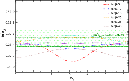
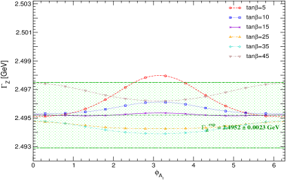
Figure 1: Prediction for $\sin^{2}\theta_{\rm eff}$ and $\Gamma_{Z}$ as function of the phase of the trilinear coupling $A_{t}$. The other SUSY parameters are: $M_{\tilde{f}}=M_{H^{\pm}}=M_{2}=m_{\tilde{g}}=500{\rm GeV},A_{\tau}=A_{t}=A_{b}=\mu=1000~{}{\rm GeV},\phi_{\mu}=\phi_{M_{1}}=\phi_{M_{2}}=\phi_{\tilde{g}}=0,\phi_{A_{b}}=0$

5 MSSM parameter scans

We now investigate the behaviour of $\sin^{2}\theta_{\rm eff}$, the $Z$ observable most sensitive to higher order corrections, by scanning over a broad range of the SUSY parameter space. The SUSY parameters given in Tab. 1 are varied independently of each other, within the given range, in a random parameter scan.

	Parameter	Range
sleptons	$M_{L_{i}},M_{E_{i}}$	$100$ to $2000~{}{\rm GeV}$
squarks	$M_{Q_{i}},M_{U_{i}},M_{D_{i}}$	$100$ to $2000~{}{\rm GeV}$
	$A_{t},A_{b}$	$-2000$ to $2000~{}{\rm GeV}$
gauginos	$M_{1},M_{2}$	$100$ to $2000~{}{\rm GeV}$
	$M_{3}$	$195$ to $1500~{}{\rm GeV}$
Higgs	$M_{A}$	$90$ to $1000~{}{\rm GeV}$
	$\tan\beta$	$1.1$ to $60$
	$\mu$	$-2000$ to $2000~{}{\rm GeV}$

Table 1: MSSM parameter ranges in the unconstrained random parameter scan shown in Figs. 2 and 3. Family indices $i$ run from $1$ to $3$, where the respective parameters are varied independently. All phases are set to zero.

Unlike Refs. mastercode ; AllanachFit ; ehoww , where our results for the electroweak precision observables were already employed in CMSSM multiparameter analyses, the scans in this section are entirely unconstrained, apart from the fact that we require the Higgs mass bounds and direct SUSY particle exclusions limits from LEP searches to hold.

The SM and the MSSM predictions for $\sin^{2}\theta_{\rm eff}$ as a function of $m_{t}$, obtained from the scatter data with $m_{t}$ as an additional free parameter, are compared in Fig. 2. The predictions within the two models give rise to two bands in the $m_{t}$–$\sin^{2}\theta_{\rm eff}$ plane with only a relatively small overlap region (indicated by a dark-shaded (blue) area). The allowed parameter region in the SM (the medium-shaded (red) and dark-shaded (blue) bands) arises from varying the only free parameter of the model, the mass of the SM Higgs boson, from $M_{H}^{\rm SM}=114$ GeV, the LEP exclusion bound LEPHiggsSM (lower edge of the dark-shaded (blue) area), to $400$ GeV (upper edge of the medium-shaded (red) area). The very light-shaded (green), the light shaded (green) and the dark-shaded (blue) areas indicate allowed regions for the unconstrained MSSM. In the very light-shaded region at least one of the ratios $m_{\tilde{t}_{2}}/m_{\tilde{t}_{1}}$ or $m_{\tilde{b}_{2}}/m_{\tilde{b}_{1}}$ exceeds 2.5 (we work in the convention that $m_{\tilde{f}_{1}}\leq m_{\tilde{f}_{1}}$), while the decoupling limit with SUSY masses of $\mathcal{O}({2})$ TeV yields the upper edge of the dark-shaded (blue) area. Thus, the overlap region between the predictions of the two models corresponds in the SM to the region where the Higgs boson is light, i.e., in the MSSM allowed region ($M_{h}\;\raisebox{-3.00003pt}{$\stackrel{{\scriptstyle\displaystyle<}}{{\sim}}$}\;130$ GeV feynhiggs ; mhiggsAEC ). In the MSSM it corresponds to the case where all superpartners are heavy, i.e., the decoupling region of the MSSM. The 68% C.L. experimental results for $m_{t}=(170.9\pm 1.8)$ GeV mt1709 and $\sin^{2}\theta_{\rm eff}$ are indicated in the plot. As can be seen from Fig. 2, the current experimental 68% C.L. region for $m_{t}$ and $\sin^{2}\theta_{\rm eff}$ is in good agreement with both models and does not indicate a preference for either of the two. The prospective accuracies for the Tevatron/LHC ($\delta\sin^{2}\theta_{\rm eff}^{\rm Tevatron/LHC}=0.00016$, $\delta m_{t}^{\rm Tevatron/LHC}=1$ GeV)) and the future ILC with GigaZ option ($\delta\sin^{2}\theta_{\rm eff}^{\rm ILC/GigaZ}=0.000013$, $\delta m_{t}^{\rm ILC/GigaZ}=0.1$ GeV) are also shown in the plot (using the current central values), indicating the strong potential for a significant improvement of the sensitivity of the electroweak precision tests gigaz (see Ref. Erler:2007sc for a recent review of the anticipated errors at future colliders).

In Fig. 3 we show the combination of $M_{W}$ MWweber and $\sin^{2}\theta_{\rm eff}$ with the top quark mass varied in the range of $165$ GeV to $175$ GeV. The ranges of the other varied parameters and the colour coding are the same as in Fig. 2. The current 68% C.L. experimental results for $M_{W}$ and $\sin^{2}\theta_{\rm eff}$ are indicated in the plot. The region of the SM prediction inside todays 68% C.L. ellipse corresponds to relatively large $m_{t}$ values, outside the current experimental range of $m_{t}=(170.9\pm 1.8)$ GeV. Thus, the combination of $M_{W}$ and $\sin^{2}\theta_{\rm eff}$ exhibits a slight preference for the MSSM over the SM. The anticipated future improvements in the measurements of $M_{W}$ and $\sin^{2}\theta_{\rm eff}$ are again indicated.

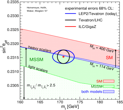
\begin{picture}(0.0,0.0) \put(0.0,0.0){} \put(0.0,0.0){} \end{picture}

Figure 2: Unconstrained MSSM random parameter scan for $\sin^{2}\theta_{\rm eff}$ as a function of $m_{t}$ over the ranges given in Tab. 1. Todays 68% C.L. level ellipses as well as future precisions, drawn around todays central value, are indicated in the plot.

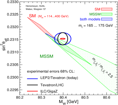
\begin{picture}(0.0,0.0) \put(0.0,0.0){} \put(0.0,0.0){} \end{picture}

Figure 3: Unconstrained MSSM random parameter scan over the ranges given in Tab. 1 and $m_{t}=165\dots 175$ GeV. Shown is the combination of $M_{W}$ and $\sin^{2}\theta_{\rm eff}$. Todays 68% C.L. level ellipses as well as future precisions, drawn around todays central value, are indicated in the plot.

References

- (1) [The ALEPH, DELPHI, L3, OPAL, SLD Collaborations, the LEP Electroweak Working Group, the SLD Electroweak and Heavy Flavour Groups], Phys. Rept. 427 (2006) 257, hep-ex/0509008; [The ALEPH, DELPHI, L3 and OPAL Collaborations, the LEP Electroweak Working Group]; M. W. Grunewald, talk given at the EPS HEP 2007 conference Manchester, England, July, 2007, arXiv:0709.3744 [hep-ph]; see also: lepewwg.web.cern.ch/LEPEWWG/Welcome.html.
- (2) D. Bardin et al., in Precision Calculations for the Resonance, Yellow report CERN 95-03, eds. D. Bardin, W. Hollik and G. Passarino; D. Bardin, M. Grünewald and G. Passarino, hep-ph/9902452.
- (3) S. Heinemeyer, W. Hollik, A.M. Weber, and G. Weiglein, arXiv:0710.2972 [hep-ph].
- (4) R. Hawkings and K. Mönig, EPJdirect C 8 (1999) 1.
- (5) S. Heinemeyer, T. Mannel and G. Weiglein, hep-ph/9909538; J. Erler, S. Heinemeyer, W. Hollik, G. Weiglein and P. Zerwas, Phys. Lett. B 486 (2000) 125; J. Erler and S. Heinemeyer, hep-ph/0102083.
- (6) O. Buchmueller et al., arXiv:0707.3447 [hep-ph].
- (7) J. Küblbeck, M. Böhm and A. Denner, Comput. Phys. Commun. 60 (1990) 165; T. Hahn, Nucl. Phys. Proc. Suppl. 89 (2000) 231; Comput. Phys. Commun. 140 (2001) 418 ;T. Hahn and C. Schappacher, Comput. Phys. Commun. 143 (2002) 54; The program is available via www.feynarts.de.
- (8) T. Hahn and M. Pérez-Victoria, Comput. Phys. Commun. 118 (1999) 153; see: www.feynarts.de/formcalc .
- (9) W. Siegel, Phys. Lett. B 84 (1979) 193; D. Capper, D. Jones and P. van Nieuwenhuizen, Nucl. Phys. B 167 (1980) 479; W. Siegel, Phys. Lett. B 94 (1980) 37; L. Avdeev, Phys. Lett. B 117 (1982) 317; L. Avdeev and A. Vladimirov, Nucl. Phys. B 219 (1983) 262; I. Jack and D. Jones, in Perspectives on Supersymmetry, ed. G. Kane (World Scientific, Singapore), p. 149; D. Stöckinger, JHEP 0503 (2005) 076.
- (10) S. Heinemeyer, W. Hollik and G. Weiglein, Comput. Phys. Commun. 124 2000 76; Eur. Phys. J. C 9 (1999) 343; The code is accessible via www.feynhiggs.de .
- (11) G. Degrassi, S. Heinemeyer, W. Hollik, P. Slavich and G. Weiglein, Eur. Phys. J. C 28 (2003) 133.
- (12) M. Frank, T. Hahn, S. Heinemeyer, W. Hollik, H. Rzehak, and G. Weiglein, JHEP 02 (2007) 047.
- (13) M. Carena, D. Garcia, U. Nierste and C. Wagner, Nucl. Phys. B 577 (2000) 577.
- (14) M. Awramik, M. Czakon and A. Freitas, JHEP 11 (2006) 048.
- (15) A. Djouadi, P. Gambino, S. Heinemeyer, W. Hollik, C. Jünger and G. Weiglein, Phys. Rev. Lett. 78 (1997) 3626. Phys. Rev. D 57 (1998) 4179, hep-ph/9710438.
- (16) J. Haestier, S. Heinemeyer, D. Stöckinger and G. Weiglein, JHEP 0512 (2005) 027.
- (17) S. Heinemeyer, W. Hollik, D. Stöckinger, A.M. Weber and G. Weiglein, JHEP 0608 (2006) 052.
- (18) B. Allanach, C. Lester, and A.M. Weber, JHEP 0612 (2006) 065; C. Allanach, K. Cranmer, C. Lester, and A.M. Weber, JHEP 0708 (2007) 023.
- (19) J. Ellis, S. Heinemeyer, K. Olive, A.M. Weber and G. Weiglein, JHEP 0708 (2007) 083.
- (20) G. Abbiendi et al. [ALEPH, DELPHI, L3, OPAL Collaborations and LEP Working Group for Higgs boson searches], Phys. Lett. B 565 (2003) 61.
- (21) Tevatron Electroweak Working Group, hep-ex/0703034.
- (22) J. Erler, (2007), hep-ph/0701261.