Study of Stability of a Charged Topological Soliton in the System of Two Interacting Scalar Fields
Abstract
An analytical-numerical analysis of the singular self-adjoint spectral problem for a system of three linear ordinary second-order differential equations defined on the entire real exis is presented. This problem comes to existence in the nonlinear field theory. The dependence of the differential equations on the spectral parameter is nonlinear, which results in a quadratic operator Hermitian pencil.
1 Introduction. Exact solution to a system of two nonlinear wave equations
The construction of precise regular solutions in systems of interacting classical fields and study of their dynamic stability are of great interest in modern nonlinear field theory [1].
In this paper, we study the problem of stability of such a solution for a system of two interacting scalar fields (this solution was reported in paper [2]), the neutral Higgs field and a charged linear field (the model was suggested in [3]). In the (1+1)-dimensional Minkowski space, the considered field system is described by the Lagrangian
| (1.1) |
Here, is a real scalar field; is a complex scalar field; and , and are real positive constants. We use the system of units where ; is the speed of light in vacuum and is the Planck constant. In this system of units, only the dimension of mass is nontrivial; the dimension of length and time is ([1], p. 13). In (1.1) , , and are dimensionless quantities, and . It is convenient to turn to the dimensionless independent variables
| (1.2) |
and introduce the new functions
| (1.3) |
In what follows, we use variables (1.2) and functions (1.3) and omit the tilde over the letters.
The system of the Lagrange-Euler equations for the Lagrangian (1.1) in terms of (1.2) and (1.3) takes the form
| (1.4) |
| (1.5) |
where is a positive dimensionless parameter and . (Here and in what follows, the asterisk denotes the Hermitian conjugation.) This system is invariant with respect to global (not depending on and ) transformations and ; for the motion integrals, it has the energy integral , charge , and topological charge defined by the formulas
| (1.6) |
| (1.7) |
| (1.8) |
Thus, the quantities and do not depend on time for those solutions of system (1.4), (1.5), for which the integrals on the right-hand sides of (1.6) and (1.7) converge, and (formula (1.8)) does not depend on for any that has finite limits as .
By definition, the invariance of Eqs. (1.4), (1.5) with respect to the transformation , where is an arbitrary real number, implies global U(1)-symmetry of these equations [1], and charge (1.7) is called a U(1)-charge.
First of all, we note that system (1.4), (1.5) is known to have the following
particular solutions:
(1) the trivial solution , , which is called a false vacuum
since it has a nonzero energy density; traveling wave solutions over the false vacuum
, , where is an arbitrary twice continuously
differentiable function (these solutions also have a nonzero energy density);
(2) solutions
| (1.9) |
with zero energy, which are reffered to as true vacua; and
(3) solutions of the domain wall type
| (1.10) |
that have the finite energy
| (1.11) |
zero charge , and the nonzero topological charge
(of course, the antiwall , is also a solution to (1.4), (1.5) with the same energy (1.11) and topological charge ).
Definition 1. A topological soliton (or a domain wall) for system (1.4), (1.5) is a solution existing and bounded in the entire space and satisfying the conditions
i.e., when has the form of a transition layer between two different vacua such that (in contrast to a nontopological soliton, when the solution tends to the same vacuum value as , i.e., when has the form of a splash over the true vacuum such that ).
In these terms, solution (1.10) is a topological soliton with zero charge .
Definition 2. A topological soliton is said to additionally bear a -charge if . Such a soliton is reffered to as a topological Q-ball (in contrast to a nontopological Q-ball with ).
The conditions for the existence of nontopological Q-balls in the Lee-Friedberg-Sirlin model [3] and their stability are discussed, along with [3], in [1] Chapter 10, and in [2]. In particular, it is shown that stable nontopological spherically symmetric and one-dimensional Q-balls for such a model exist for large values of the charges, , where is a critical charge depending on the parameters of the Lagrangian. However, the explicit form of such Q-balls has not yet been found.
In [2], for system (1.4), (1.5), the following precise solution of the topological Q-ball type was found:
| (1.12) |
| (1.13) |
For this configuration, from (1.6) – (1.8), we obtain
| (1.14) |
| (1.15) |
| (1.16) |
Remark 1. It follows from the above discussions, that the functions and are also solutions to system (1.4), (1.5) with the same , , and .
Remark 2. Taking into account the invariance of Eqs. (1.4), (1.5) with respect to the Lorentz transformations of the independent variables and , we find that solution (1.10) generates for Eq. (1.5) (for ) the traveling wave front if an initial speed : , is given; solution (1.12), (1.13) generates for system (1.4), (1.5) the traveling wave of the form , with oscillations in the -component.
In conclusion of this section, we briefly discuss physical interpretation (in addition to that in [2]) of solution (1.12), (1.13). This solution possesses properties similar to those of possible Q-balls [4] in the (3+1)-dimensional Minkowski space, which are assumed to have something to do with the problem of the baryon asymmetry of the Universe. One of the mechanisms that can explain the baryon asymmetry has been suggested in [5]. In accordance with this mechanism, at the late inflation stages, a condensate is formed that can evolve into Q-balls that bear the same baryon charge but are more advantageous from the energy standpoint. Note that these Q-balls may continue to exist until now and contribute to the dark matter. Moreover, it has been noted in [6] that such ”relict” Q-balls may occur crucial factors when studying stability of neutron stars.
The precise solution of the Q-ball type in the (1+1)-dimensional Minkowski space, which was found in [2] and is studied in this paper, is important not only as an approximation of (3+1)-dimensional Q-balls; it is of great interest in connection with studying domain walls and processes on them.
2 Dynamic stability of the solution and spectral problem statement
From the standpoint of physical applications, the problem of the dynamic stability of solution (1.12), (1.13) is of great importance. A solution is considered to be absolutely stable if the energy functional takes its absolute minimum on this solution. For system (1.4), (1.5) true vacua (1.9) are solutions of this kind. However, these solutions possess zero - and -charges.
Definition 3. A solution , to system (1.4), (1.5) is said to be absolutely stable in a sector if it has the least energy among all solutions with fixed values of charges (1.7) and (1.8).
Solution (1.10) is absolutely stable in the sector , since it is the only stationary solution of system (1.4), (1.5) in this sector.
The question of whether solution (1.12), (1.13) is absolutely stable in the sector , where and are defined by (1.15) and (1.16), respectively, is not easy to answer because of the dependence of component (1.13) on time.
A suggestive consideration regarding the stability of solution (1.12), (1.13) might be as follows: the parameter affects only the amplitude in (1.13); for , solution (1.12), (1.13) turns to the absolutely stable solution (1.10); and, for , there appears a nonzero -charge, which usually only stabilizes the solution (see [1], Chapter 10).
The main part of this paper is devoted to studying the dynamic stability of solution (1.12), (1.13) with respect to small perturbations (Lyapunov’s stability in the framework of linear theory). However, first, we present some physical considerations regarding the stability of configuration (1.12), (1.13) from the standpoint of its possible disintegration into charged nonlocalized formations.
1. The problem consists in searching for possible solutions in the sector that are close to solution (1.10), which is absolutely stable in the sector . The solutions are sought in the form of small nonlocalized perturbations of the field determining the charge . Such solutions, if they exist, may occur equivalent to or more advantageous than solution (1.12), (1.13) from the energy considerations. An approximate solution to system (1.4), (1.5) close to (1.10) is sought in the form , where and
| (2.1) |
i.e., only the -component in (1.10) is perturbed. From (1.4), we obtain the following equation in :
| (2.2) |
To separate variables in (2.2), the solution is sought in the form
| (2.3) |
where is a separation parameter and satisfies the ODE
| (2.4) |
For reasons that will be clear from the following discussions, we assume that the solution is defined in an arbitrarily large but still finite interval . From (1.6) and (1.7), we obtain the following expressions for the charge and energy of solution (2.3):
| (2.5) |
| (2.6) |
In the interval , Eq. (2.4) may have only a descrete spectrum. If is an eigenvalue from the discrete spectrum, the corresponding eigenfunction belongs to and has the following asymptotics for large :
| (2.7) |
where is a normalization constant. Since the perturbation must be normalized by the given charge , the localized eigenfunction with asymptotics (2.7) does not generally meet the requirement of the perturbation smallness for large .
The values belong to the continuous spectrum. If is an eigenfunction corresponding to an eigenvalue belonging to the continuous spectrum, it has the following asymptotics for large :
| (2.8) |
where the phase is uniquely determined by the boundary condition at , either or , and the amplitude is the normalization constant. If normalization (2.5) is used, the amplitude may be selected as small as desired through an appropriate choice of . In addition, for , so that the least value for (2.6) is obtained when in (2.8). Since, in the framework of the approximation considered, integrals (1.6) and (1.7) with the infinite limits diverge on solutions (2.1), (2.3), and (2.8) for , the function is set equal to zero outside some arbitrarily large (but finite) interval . Note that this expedient is often used when solving physical problems (see, for example, [7], pp. 170-174; [1], Chapter 10.)
Let us multiply (2.4) by and integrate the equation obtained in the interval . In so doing, the term is integrated by parts with regard to the conditions . As a result, we obtain
From this and (2.6), we have
Hence, with regard to (2.5), it follows that
| (2.9) |
for . Finally, we find that the energy of the configuration composed of the domain wall (2.1) with charged perturbations (2.3) over it is the sum of and given by (1.11) and (2.9), respectively; i.e.,
| (2.10) |
Note that the energy and charge of the precise solution (1.12), (1.13) are uniquely specified by the parameters of Lagrangian (1.1). At the same time, in the linear approximation, configuration (2.1), (2.3) may have arbitrary and satisfying (2.10).
Inequality (2.10) can be derived in a different way. Since the domain wall (2.1) is localized on the interval of length , to compute the energy of nonlocalized perturbations of the field , we substitute and into Eq. (1.4), which implies the perturbation of vacua (1.9) along the component (here, we rely on the physically reasonable assumption that the field is concentrated basically outside the domain where the wall is localized). For the function , we obtain the equation (cf. with (2.2))
| (2.11) |
In order to avoid diverging integrals in the computation of the energy and charge, we again consider the perturbations on a large, but finite, interval . Among solutions of Eq. (2.11) corresponding to a given charge , the normalized solution
| (2.12) |
has the least energy (note that this solution does not depend on ). Here, the normalization multiplier is determined from the condition that the U(1)-charge for the field is equal to , i.e.,
The energy of solution (2.12) is equal to . Adding together this quantity and the wall energy (1.11), we obtain the expression coinciding with the right-hand side of (2.10).
For the precise solution (1.12), (1.13), we obtain from (1.14) and (1.15) the following relationship between the charge and energy:
| (2.13) |
It is easy to see from (2.10) and (2.13) that, for any admissible values of the parameter , the energy of the precise solution is less than the minimal possible energy of the nonlocalized configuration (2.1), (2.3) with the same charge. This brings us to the conclusion that solution (1.12), (1.13) is stable in terms of the disintegration into a nonlocalized configuration of the type ”wall + plane waves”.
2. The basic objective of this work is to study the dynamic stability of solution (1.12), (1.13) in the framework of linear perturbation theory. We use the approach similar to that employed in studying the stability of localized solutions of some nonlinear wave equations in field theory [8] – [10]. In particular, it was used in [10] for studying the stability of a precise nontopological soliton carrying a U(1)-charge for a complex wave equation with fifth-degree nonlinearity.
Let us set and , where and are small deviations from (1.12), (1.13); note that is a real-valued function and is a complex-valued function. System (1.4), (1.5) reduces to the following linearized system of the differential equations in the deviations:
| (2.14) |
| (2.15) |
Similarly [8] – [10], the solution to Eqs. (2.14), (2.15) is sought in the form
| (2.16) |
| (2.17) |
Such a representation of the solution makes it possible to separate variables in (2.14), (2.15) and to obtain ODEs for the amplitudes of the perturbations , and not depending on . Indeed, substituting (1.12), (1.13), (2.16), and (2.17) into (2.14) and (2.15), we obtain the following system of ODEs for , , and depending on the parameter :
| (2.18) |
| (2.19) |
| (2.20) |
Solutions to system (2.18) – (2.20) are sought in the class of square integrable functions defined on the entire real axis satisfying the conditions
| (2.21) |
It is required to find the values of (eigenvalues) for which the singular boundary value problem (2.18) – (2.21) has nontrivial solutions (eigenfunctions). By virtue of (2.16), (2.17), for any complex eigenvalue with a nonzero imaginary part, the perturbations grow exponentially in time. Hence, the dynamic stability of solution (1.12), (1.13) with respect to small perturbations of form (2.16), (2.17) requires that the discrete spectrum of problem (2.18) – (2.21) be real.
3 Analytic properties of the spectral problem
Taking into account that the ODE system (2.18) – (2.20) is not changed upon the replacement of (, , , ) by (, , , ) or (, , , ), we can consider the singular boundary value problem on the semiaxis and write it in the following final form:
| (3.1) |
| (3.2) |
| (3.3) |
| (3.4) |
| (3.5) |
| (3.6) |
| (3.7) |
This problem contains terms depending nonlinearly on the spectral parameter and, generally, may have complex eigenvalues. We seek for nontrivial solutions to this problem in the class of complex-valued functions satisfying the condition
| (3.8) |
Note that the singular boundary value problem (3.1) – (3.7) is correctly defined in terms of the number of the boundary conditions for large if and only if the singular Cauchy problem (3.1) – (3.3), (3.5) – (3.7) admits a three-parameter family of solutions at infinity. Since system (3.1) – (3.3) is asymptotically equivalent to a system with constant coefficients, each of the decoupled second-order ODE for large must have a one-parameter family of solutions vanishing at infinity. This results in the following requirements on the location of the eigenvalues in the complex plane:
| (3.9) |
i.e., they do not lie on the nonpositive real semiaxis. Then, for sufficiently large , , the three-dimensional linear subspace generated in the phase space C6 of system (3.1) – (3.3) by the values of the solutions of the singular Cauchy problem (3.1) – (3.3), (3.5) – (3.7) is given in the form
| (3.10) |
| (3.11) |
| (3.12) |
where the roots are assumed to have positive real parts (see [11] for detail).
Hence, the following assertions are valid:
(1) real eigenvalues of problem (3.1) – (3.8), if exist, satisfy (by virtue of (3.9)) the inequalities
| (3.13) |
(2) the geometric multiplicity of any eigenvalue of problem (3.1) – (3.8) cannot be greater than three; i.e., not more than three linearly independent eigenfunctions may correspond to one eigenvalue;
(3) system (3.1) – (3.3) has a continuous spectrum lying on the real axis of the complex plane in the intervals and (conditions (3.10), (3.11), and (3.12) turn to conditions of the radiation type for and , for and , and for , respectively); these real intervals of the continuous spectrum do not affect stability of solution (1.12), (1.13) with respect to small perturbations of form (2.16), (2.17).
Note also that, if is a purely imaginary eigenvalue of problem (3.1) – (3.8), then , and is a real-valued function.
These assertions can be supplemented by the following facts and estimates.
1. Case of =2. For , system (3.1) – (3.3) is decoupled into the three second-order ODEs:
| (3.14) |
| (3.15) |
| (3.16) |
each of which can be reduced to a hypergeometric equation. Indeed, consider the equation
| (3.17) |
and introduce the change of variable . For the function , we obtain the equation
which reduces to a hypergeometric equation by means of the substitution and the change of variable . Assuming that , we obtain
| (3.20) |
This equation has the two independent integrals [12]:
where is the hypergeometric function
Hence, returning to (3.17), we obtain
Then, only belongs to under the condition that and , where , when becomes a polynomial of the -th degree in and, hence, has finite limits as .
For example, for Eq. (3.14), we have , and . Hence, it follows that , , , and . Equations (3.15) and (3.16) are treated in a similar way. Hence, in the case of , all points of the discrete spectrum of problem (3.1) – (3.8) and all eigenfunctions corresponding to them can be found (all eigenfunctions are accurate up to the normalizing multipliers):
| (3.21) |
| (3.22) |
| (3.23) |
Thus, for , the eigenvalue of problem (3.1) – (3.8) has the maximal possible geometric multiplicity equal to three, whereas the multiplicity of the eigenvalues , , , and is equal to one.
2. Case of 0¡¡2. It is easy to check that, for any satisfying the inequalities , remains an eigenvalue of problem (3.1) – (3.8), and there are, at least, two eigenfunctions corresponding to it; namely,
| (3.24) |
| (3.25) |
Note further that, if is a solution to problem (3.1) – (3.8), then , and are also its solutions, so that it is sufficient to consider, for example, the following range of :
| (3.26) |
Like in [8] – [10], we write system (3.1) – (3.3) in the form
| (3.27) |
where ( denotes the transposition) and , , and are operators defined in the space of three-component complex-valued twice differentiable functions bounded on the semiaxis and satisfying conditions (3.4) – (3.8), : , with the scalar product defined as
Here, is the identity operator and and have the form
| (3.28) |
where
| (3.29) |
Taking the scalar product of (3.27) with and assuming that is normalized such that ), we obtain
| (3.30) |
and are Hermitian operators. The operator is obviously Hermitian; is Hermitian because the operator is Hermitian. The latter follows from the fact that the substitutions and turn to zero on the functions satisfying conditions (3.4) – (3.7). Then, and are real numbers. From (3.30), it follows that
| (3.31) |
From this equation, we can obtain estimates for an eigenvalue with a nonzero imaginary part. Indeed, in this case, it follows from (3.31) that
| (3.32) |
We have the following estimates for the real and imaginary parts of :
| (3.33) |
| (3.34) |
where is the least eigenvalue of the operator . Let us obtain an estimate for . From (3.28), (3.29), we have
We estimate for the first integral is obtained by dropping the positive terms:
| (3.35) |
Taking into account that , we obtain the estimate for the second integral
| (3.36) |
Further, applying the transformation
| (3.37) |
and noting that it is unitary (does not change the value of the scalar product , we obtain
| (3.38) |
From (3.36) and (3.38), we obtain
From this inequality and (3.35), it follows that
| (3.39) |
Using (3.32) – (3.34) and (3.39), we finally obtain the following estimates:
| (3.40) |
| (3.41) |
4 Numerical study of stability
4.1 Refiniment of the localization domain for the eigenvalues of problem (3.1) – (3.8)
Along with analytic estimates (3.40), (3.41), the localization domain for the eigenvalues of problem (3.1) – (3.8) can be determined numerically starting from the estimate
| (4.1) |
To find the numbers , we consider an accompanying eigenvalue problem for the operator (see (3.28), (3.29)), i.e., the -parameterized ODE system
| (4.2) |
subject to the boundary conditions (3.4) – (3.7) and requirement (3.8).
In order to solve this problem numerically, it should be reduced to a problem defined on a finite interval. As noted in Section 3, the condition that the solutions belong to the space is equivalent to the requirement that the values of the solutions for large belong to a three-dimensional subspace of , which, up to exponentially small terms, is defined as
| (4.3) | |||
| (4.4) | |||
| (4.5) |
Problem (4.2), (3.4), (4.3)–(4.5) is self-adjoint. Taking into account item 1 of Section 3, we immediately find that, for , is its only eigenvalue (of multiplicity 3), and that the corresponding eigenfunctions are given by (3.21) – (3.23). For different from , the eigenvalue has multiplicity 2, with the corresponding eigenfunctions being given by (3.24) and (3.25), and, as computations show, the third zero eigenvalue starts to move to the region of negative values. The eigenvalue is sought numerically by transferring boundary conditions (4.3) – (4.5) from the point to the point and examining the changes of sign of the resulting determinant. Note that, in this case, a variant of the sweep method is used [13] (with regard to the studies on the robust use of orthogonal sweep methods in singular problems [14]).
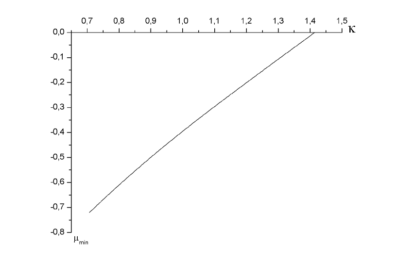
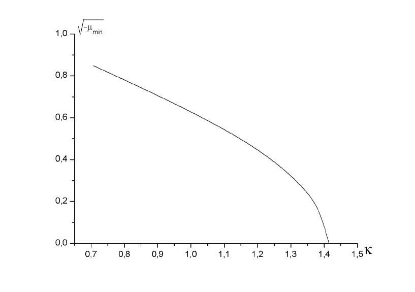
Our computations show that, when varies from to zero, the double zero eigenvalue remains unchanged, whereas the single eigenvalue (which is just the eigenvalue we are interested in) moves to the region of negative values (Fig. 1). The comparison of these results with (3.39) shows that the bound obtained analytically is too high. For example, for , the value of found numerically is equal to 0.45, whereas (3.39) yields 1.8. Nevertheless, for , the magnitude of is greater than (see estimate (3.13) and Fig. 2), which complicates the localization of the eigenvalues of problem (3.1)–(3.8) (see below).
4.2 Search for eigenvalues of problem (3.1) – (3.8) in the sector (4.1), (3.26)
Now, let us consider problem (3.1) – (3.8) itself. Its reduction to a problem defined on a finite interval is similar to that for the previous problem for the ODE (4.2). Representation (3.10) – (3.12) yields the following boundary conditions at :
| (4.6) |
| (4.7) |
| (4.8) |
where the roots are assumed to have positive real parts.
The nonsingular spectral problem (3.1) – (3.4), (4.6) – (4.8) was studied numerically by a method based on the generalization of the argument principle (methods of localization of descrete spectrum points based on the argument principle and its modifications are discussed, for example, in [15] – [18] and in references therein) with the use of the differential sweep [13] (as noted earlier, the problems of the robust application of the method from [13], as well as other modifications of the sweep method, to singular eigenvalue problems are discussed in [14]). Conditions (4.6) – (4.8) are represented in the form
| (4.9) |
where and
| (4.10) |
As a result of the sweep, we obtain a condition at the point with the matrix equivalent to (4.9), (4.10). If we augment thi matrix up to a square one by adding the lower matrix block corresponding to conditions (3.4), eigenvalue problem can be formulated as follows:
a number is an eigenvalue the determinant
of the resulting matrix is equal to zero;
the geometric multiplicity of an eigenvalue (i.e., the number of linear
independent eigenfunctions) is equal to the defect of the resulting
matrix.
Note that the coefficients of the matrix and, hence, the determinant of the resulting matrix, are not analytic functions of . Nevertheless, as shown in [16], the argument principle can still be used for determining the number of the eigenvalues in a given region of the spectral parameter . The search can rely on the determinants for the first condition and for the second condition in (3.4), respectively, where is the minor of the matrix composed of the columns , , and . The zeros of det correspond to the eigenvalues of problem (3.1) – (3.4), (4.6) – (4.8). The algebraic multiplicity of an eigenvalue is the multiplicity of the corresponding zero of the determinant.
From the computational results, it follows that when is close to , the search domain for unstable eigenvalues is a circle of radius centered at the origin (see (4.1)). When approaches zero, the search domain is the same circle with the cuts along the real axis from to the right and from to the left (see (3.13)).
The critical difficulty associated with this problem is that the points lying on the cuts belong to the continuous spectrum (when is close to the cuts, the computation becomes unstable). Thus, the methods of the localization of the eigenvalues described in [15]–[18] cannot directly be applied to our problem, since the resulting determinant (or some other function used in the argument principle) cannot continuously be extended to the boundary of the domain. (Note only that, if there were descrete eigenvalues appearing in the intervals of the continuous spectrum, they would develop somehow when varies; however, the computation did not reveal anything of this kind near the cuts when varied.)
From the problem symmetry, it follows that the eigenvalues with nonzero real and imaginary parts are located in the complex -plane by quadruplets () and those with only real or imaginary nonzero parts, by pairs on the real or imaginary axis, respectively.
To study perturbations of the degenerate eigenvalue and reveal the presence / absence of complex eigenvalues, we made computations on the following contours in the -plane:
circles of radius varying from to , where is a small number, centered at ;
circular sectors of the angle 900 with the vertex at and radius located in the first quadrant (the eigenvalue symmetry property is used);
intervals lying on the real or imaginary axis;
separate contours outside the real axis.
The computations show that, in the degenerate case of , the algebraic multiplicity of the eigenvalue is equal to four, and its geometric multiplicity is equal to three (cf. with (3.21) – (3.23)). The difference in the two multiplicities is explained not by the presence of Jordan block (which is impossible in view of the self-adjointness of the boundary value problem) but by the fact that Eq. (3.3) contains the square of the spectral parameter .
When varies from to 0, the following picture is observed. As before, the algebraic multiplicity of the eigenvalue is equal to 4. Thus, we may conclude that the eigenvalue is not split into several eigenvalues. Moreover, when is close to , it follows from the results obtained that the problem has no other eigenvalues. When we move from , the geometric multiplicity reduces from 3 to 2 (instead of eigenfunctions (3.22), (3.23) we have (3.24)). The reduction of the geometric multiplicity upon the perturbation of a parameter is a typical phenomenon for quadratic pencils (in contrast to linear ones). Eigenfunctions (3.21) – (3.23) for and (3.24), (3.25) for other are found numerically with accuracy up to . As approaches zero, problem (3.1) – (3.8) becomes more stiff. In the computations with fixed (double) relative accuracy, the lowest value of was as small as 0.05.
For additional stability control for the eigenvalue , we used the following consideration. From the symmetry of the eigenvalues and the existence of the eigenfunctions (3.24), (3.25), it follows that, at least, the property of being repeated for the eigenvalue is conserved. Hence, the perturbation could accur only through splitting of two symmetric eigenvalues along one of the axis. We have checked numerically that this effect did not take place (with regard to estimates (3.13) and (3.41)). No other eigenvalues have been found in the numerical experiments.
It may be concluded (with the greatest certainty for the interval : ) that the singular boudary value problem, (3.1) – (3.8) has only one eigenvalue of algebraic multiplicity 4 and geometric multiplicity 2 with the corresponding eigenfunctions (3.24), (3.25). No complex eigenvalues have been found in the admissible domain (4.1).
5 Conclusions
The analytical and numerical studies reported in this paper allow us to conclude that solution (1.12), (1.13) is dynamically stable with respect to small perturbations of form (2.16), (2.17) for . This statement has the greatest certainty in the interval : . Moreover, solution (1.12), (1.13) in the course of its evolution cannot split into small nonlocalized oscillations (along the component ) over kink (1.10) since it is not advantageous from the energy standpoint. The question of whether the topological Q-ball (1.12), (1.13) is absolutely stable in the sector is still open.
6 Acknowledgments
This work was supported by the Russian Foundation for Basic Research, projects 02-01-00050 and 00-15-96562. We also acknowledge the support of the Federal Agency of Atomic Energy of the Russian Federation.
We are grateful to A. A. Abramov, N. A. Voronov, A. E. Kudryavtsev and S. P. Popov for discussion of this work and usefull comments.
References
- [1] V. A. Rubakov, Classical Gauge Fields. Editorial URSS, Moscow, 1999.
- [2] V. A. Lensky, V. A. Gani, A. E. Kudryavtsev, ”On Domain Walls Carrying U(1)-charge”, Zh. Eksp. Teor. Fiz. 120, 778-785 (2001).
- [3] R. Friedberg, T. D. Lee, A. Sirlin, ”Class of scalar-field soliton solutions in three space dimensions”, Phys. Rev. D 13, pp. 2739-2761 (1976).
- [4] S. Coleman, ”Q-balls”, Nucl. Phys. B 262, pp. 263-283 (1985).
- [5] I. Affleck, M. Dine, ”A new mechanism for baryogenesis”, Nucl. Phys. B 249, pp. 361-380 (1985).
- [6] A. Kusenko, M. Shaposhnikov, P. Tinyakov, I. Tkachev, ”Star wreck”, Phys. Lett. B 423, pp. 104-108 (1998).
- [7] L. D. Landau, E. M. Lifshitz, Course of Theoretical Physics, Vol. 2: The Classical Theory of Fields (Nauka, Moscow, 1988; Pergamon, Oxford, 1975).
- [8] D. L. T. Anderson, G. H. Derrick, ”Stability of time-dependent particlelike solution in nonlinear field theories. I”, J. Math. Phys. 11 (4), pp. 1336-1346 (1970).
- [9] D. L. T. Anderson, ”Stability of time-dependent particlelike solution in nonlinear field theories. II”, J. Math. Phys. 12 (6), pp. 945-952 (1971).
- [10] T. I. Belova, N. A. Voronov, N. B. Konyukhova, and B. S. Pariiskii, ”Stability Domains of One-Dimensional Solitons of a Charged Scalar Field”, Yadernaya Fiz., 57 (11), pp. 2105-2112 (1994).
- [11] E. S. Birger, N. B. Lyalikova (Konyukhova), ”Solutions of Some Systems of Ordinary Differential Equations Satisfying Given Conditions at Infinity”, Zh. Vychisl. Mat. Mat. Fiz. 5 (5), pp. 979-990 (1965).
- [12] N. N. Lebedev, Special Functions and Their Applications, 2nd ed. (Fizmatgiz, Moscow, 1963; Prentice-Hall, Englewood Cliffs, 1965).
- [13] A. A. Abramov, ”Transferring Boundary Conditions for Systems of Linear Ordinary Differential Equations (Sweep Method)”, Zh. Vychisl. Mat. Mat. Fiz. 1 (3), pp. 542-545 (1961).
- [14] A. A. Abramov, V. V. Ditkin, N. B. Konyukhova, et al., ”Computation of Eigenvalues and Eigenfunctions for Ordinary Differential Equations with Singularities”, Zh. Vychisl. Mat. Mat. Fiz. 20 (5), pp. 1155-1172 (1980).
- [15] S. V. Kurochkin, ”A Method for Finding Eigenvalues of a Non-self-adjoint Boundary Value Problem”, Dokl. Akad. Nauk, 336 (4), pp.442-443 (1994).
- [16] A. A. Abramov and L. V. Yukhno, ”On the Determination of Number of Eigenvalues of a Spectral Problem”, Zh. Vychisl. Mat. Mat. Fiz. 34 (5), pp. 776-783 (1994).
- [17] S. V. Kurochkin, ”Topological Methods for Localizing Eigenvalues of Boundary Value Problems”, Zh. Vychisl. Mat. Mat. Fiz. 35 (8), pp. 1165-1174 (1995).
- [18] A. A. Abramov, V. I. Ul’yanova, and L. V. Yukhno, ”On the Application of the Argument Principle in a Spectral Problem for Systems of Ordinary Differential Equations with Singularities”, Zh. Vychisl. Mat. Mat. Fiz. 38 (1), pp. 61-67 (1998) [Comp. Math. Math. Phys. 38, pp. 57-63 (1998)].