Abstract

We present the currently most accurate prediction of $Z$ pole observables such as $\sin^{2}\theta_{\mathrm{eff}}$, $\Gamma_{Z}$, $R_{b}$, $R_{l}$, and $\sigma^{0}_{\rm had}$ in the Minimal Supersymmetric Standard Model (MSSM). We take into account the complete one-loop results including the full complex phase dependence, all available MSSM two-loop corrections as well as the full SM results. We furthermore include higher-order corrections in the MSSM Higgs boson sector, entering via virtual Higgs boson contributions. For $\Gamma(Z\to\tilde{\chi}^{0}_{1}\tilde{\chi}^{0}_{1})$ we present a full one-loop calculation. We analyse the impact of the different sectors of the MSSM with particular emphasis on the effects of the complex phases. The predictions for the $Z$ boson observables and $M_{W}$ are compared with the current experimental values. Furthermore we provide an estimate of the remaining higher-order uncertainties in the prediction of $\sin^{2}\theta_{\mathrm{eff}}$.

1 Introduction

$Z$ boson physics is well established as a cornerstone of the Standard Model (SM) [1, 2, 3]. Many (pseudo-) observables [4] have been measured with high accuracy using the processes (mediated at lowest order by photon and $Z$ boson exchange)

$$e^{+}e^{-}\to f\bar{f},\ \ \ \ \ f\neq e,$$ (1)

at LEP and SLD with a center of mass energy $\sqrt{s}\approx M_{Z}$. In particular these are the effective leptonic weak mixing angle at the $Z$ boson resonance, $\sin^{2}\theta_{\mathrm{eff}}$, $Z$ boson decay widths to SM fermions, $\Gamma(Z\to f\bar{f})$, the invisible width, $\Gamma_{\rm inv}$, the total width, $\Gamma_{Z}$, the ratios of partial widths, $R_{l}$ and $R_{b}$, forward-backward and left-right asymmetries, $A_{\rm FB}$ and $A_{\rm LR}$, and the total hadronic cross section, $\sigma^{0}_{\rm had}$. Together with the measurement of the mass of the $W$ boson, $M_{W}$, and the mass of the top quark, $m_{t}$, the $Z$ pole observables have been used to constrain indirectly the SM Higgs boson mass, $M^{\textup{SM}}_{H}$, the last free parameter of the model, yielding $M^{\textup{SM}}_{H}=76^{+33}_{-24}\,\,\mathrm{GeV}$ with an upper limit of $M^{\textup{SM}}_{H}\leq 144\,\,\mathrm{GeV}$ at the 95% C.L. [1, 2]. The precision observables are also very powerful for testing models beyond the SM. In particular the Minimal Supersymmetric Standard Model (MSSM) [5] has been investigated, see Ref. [6] for a review. Performing fits in constrained SUSY models a certain preference for not too heavy SUSY particles has been found [7, 8, 9, 10, 11, 12]. The prospective improvements in the experimental accuracies, in particular at the ILC with GigaZ option, will provide a high sensitivity to deviations both from the SM and the MSSM.

In order to fully exploit the high-precision measurements, the theoretical uncertainty in the predictions of the (pseudo-) observables should be sufficiently smaller than the experimental errors. Within the SM the complete one-loop and two-loop results [13, 14, 15, 16] as well as leading higher-order contributions [17, 18, 19, 20, 21] are available for $\sin^{2}\theta_{\mathrm{eff}}$. For the leptonic and hadronic $Z$ widths partial results for process-specific two-loop corrections are known [4, 22, 23, 24].

The theoretical evaluation of the $Z$ pole observables within the MSSM is not as advanced as in the SM. So far, the one-loop contributions have been evaluated completely, restricted however to the special case of vanishing complex phases (contributions to the $\rho$ parameter with non-vanishing complex phases in the scalar top and bottom mass matrices have been considered in Ref. [25]). At the two-loop level, the leading ${\cal O}(\alpha\alpha_{s})$ corrections [26] and the leading electroweak corrections of ${\cal O}(\alpha_{t}^{2})$, ${\cal O}(\alpha_{t}\alpha_{b})$, ${\cal O}(\alpha_{b}^{2})$ to $\Delta\rho$ have been obtained [27, 28] ($\alpha_{t}$ and $\alpha_{b}$ are defined in terms of the Yukawa couplings $y_{f}$ as $\alpha_{f}=\frac{y_{f}^{2}}{4\pi}$). Going beyond the minimal SUSY model and allowing for non-minimal flavor violation the leading one-loop contributions to $\Delta\rho$ are known [29].

In order to confront the predictions of supersymmetry (SUSY) with the electroweak precision data and to derive constraints on the supersymmetric parameters, it is desirable to achieve the same level of accuracy for the SUSY predictions as for the SM. In this paper we present complete one-loop results for the $Z$ boson observables in the MSSM with complex parameters, taking into account the full complex phase dependence. Besides the decays of the $Z$ boson into quarks and leptons, we also provide a complete one-loop result for the partial width of the $Z$ boson decay into the lightest neutralino, $\Gamma(Z\to\tilde{\chi}^{0}_{1}\tilde{\chi}^{0}_{1})$, which is the first one-loop result for this decay in the full MSSM. If the $Z$ boson decay into the lightest neutralino is kinematically possible it contributes to the invisible width of the $Z$ boson. We combine our new one-loop results with the full set of available higher-order corrections in the MSSM. In order to recover the state-of-the-art SM results in the decoupling limit where all supersymmetric particles are heavy, we consistently incorporate also those SM-type higher-order corrections which go beyond the results obtained within the MSSM so far. In this way we provide the currently most complete results for the $Z$ boson observables in the MSSM (for the corresponding results for the $W$ boson mass, $M_{W}$, see Ref. [30]). A public computer code based on our result for the electroweak precision observables (EWPO), i.e. the $Z$ pole observables and $M_{W}$, is in preparation [31]. It provides predictions for the EWPO in terms of the low-energy parameters of the MSSM, which can be freely chosen as independent inputs.

We analyse the numerical results for the EWPO for various MSSM scenarios, such as SPS benchmark scenarios [32], scenarios with heavy scalar masses [33, 34] and the CPX scenario [35]. The dependence of the results for the EWPO on the complex phases is investigated. For $\sin^{2}\theta_{\mathrm{eff}}$, showing the largest sensitivity of the $Z$ pole observables to the SUSY loop corrections, we provide an estimate of the remaining theoretical uncertainties from unknown higher-order corrections.

The rest of the paper is organised as follows: In Sect. 2 we introduce our notations and conventions. The $Z$ pole observables are discussed in Sect. 3. Details about the evaluation of the higher-order corrections are given in Sect. 4. In Sect. 5 we present our numerical analysis. The estimate of the theory uncertainties in the prediction for $\sin^{2}\theta_{\mathrm{eff}}$ from unknown higher-order corrections is given in Sect. 6. We conclude with Sect. 7.

2 Notations and conventions

In the complex MSSM, the $Z$ pole observables depend on all the free parameters of the model, such as SUSY particle masses, mixing angles and couplings. In order to be self-contained we list in this section the notations and conventions used in our calculations. We briefly describe the relevant quantities in the sfermion, the chargino/neutralino, and the Higgs boson sector of the MSSM.

2.1 Sfermions

The mass matrix for the two sfermions of a given flavour, in the $\tilde{f}_{L},\tilde{f}_{R}$ basis, is given by

$${{\mathbf{M}}}_{\tilde{f}}=\begin{pmatrix}M_{L}^{2}+m_{f}^{2}&m_{f}\;X_{f}^{*}\\ m_{f}\;X_{f}&M_{R}^{2}+m_{f}^{2}\end{pmatrix},$$ (2)

with

$$M_{L}^{2} = M_{\tilde{F}}^{2}+M_{Z}^{2}\cos 2\beta\hskip 2.84526pt(I^{f}_{3}-Q_{f}s_{\mathrm{w}}^{2}),$$

$$M_{R}^{2} = M_{\tilde{F}^{\prime}}^{2}+M_{Z}^{2}\cos 2\beta\hskip 2.84526ptQ_{f}s_{\mathrm{w}}^{2},$$ (3)

$$X_{f} = A_{f}-\mu^{*}\{\cot\beta\hskip 2.84526pt,\tan\beta\},$$

where $\{\cot\beta\hskip 2.84526pt,\tan\beta\}$ applies for up- and down-type sfermions, respectively, and $\tan\beta$ is the ratio of the two vacuum expectation values of the two Higgs doublets (see Sect. 2.3), $\tan\beta\equiv v_{2}/v_{1}$. We have furthermore used $s_{\mathrm{w}}^{2}\equiv\sin^{2}\theta_{\rm W}=1-M_{W}^{2}/M_{Z}^{2}$. In the Higgs and scalar fermion sector of the complex MSSM, $N_{f}+1$ phases are present, one for each $A_{f}$ and one for $\mu$, i.e. $N_{f}+1$ new parameters appear in comparison to the MSSM with only real parameters. As an abbreviation,

$$\phi_{A_{f}}\equiv\arg(A_{f})\,$$ (4)

will be used. As an independent parameter one can trade $\phi_{A_{f}}$ for $\phi_{X_{f}}\equiv\arg(X_{f})$. The sfermion mass eigenstates are obtained by the transformation

$$\left(\begin{array}[]{c}\tilde{f}_{1}\\ \tilde{f}_{2}\end{array}\right)={{\mathbf{U}}_{\tilde{f}}}\left(\begin{array}[]{c}\tilde{f}_{L}\\ \tilde{f}_{R}\end{array}\right),$$ (5)

with a unitary matrix ${\mathbf{U}}_{\tilde{f}}$. The mass eigenvalues are given by

$$m_{\tilde{f}_{1,2}}^{2}=m_{f}^{2}+\frac{1}{2}\left[M_{L}^{2}+M_{R}^{2}\mp\sqrt{(M_{L}^{2}-M_{R}^{2})^{2}+4m_{f}^{2}|X_{f}|^{2}}~{}\right],$$ (6)

and are independent of the phase of $X_{f}$.

2.2 Gaugino sector

The physical masses of the charginos are determined by the matrix

$${\mathbf{X}}=\begin{pmatrix}M_{2}&\sqrt{2}\sin\beta\,M_{W}\\ \sqrt{2}\cos\beta\,M_{W}&\mu\end{pmatrix},$$ (7)

which contains the soft breaking term $M_{2}$ and the Higgsino mass term $\mu$, both of which may have complex values in the complex MSSM. Their complex phases are denoted by

$$\phi_{M_{2}}\equiv{\rm arg}\left(M_{2}\right)\ \ \ \ \ \textup{and}\ \ \ \ \ \phi_{\mu}\equiv{\rm arg}\left(\mu\right).$$ (8)

The physical masses are denoted as $m_{\tilde{\chi}^{\pm}_{1,2}}$ and are obtained by applying the diagonalisation matrices ${{{\mathbf{U}}}_{{\tilde{\chi}}^{\pm}}}$ and ${{{\mathbf{V}}}_{{\tilde{\chi}}^{\pm}}}$

$${\bf U^{\ast}_{{\tilde{\chi}}^{\pm}}}{\mathbf{X}}{{{\mathbf{V}}}^{\dagger}_{{\tilde{\chi}}^{\pm}}}=\textup{diag}\left(m_{\tilde{\chi}^{\pm}_{1}},m_{\tilde{\chi}^{\pm}_{2}}\right).$$ (9)

The situation is similar for the neutralino masses, which can be calculated from the mass matrix ($s_{\mathrm{w}}=\sin\theta_{\rm w}$, $c_{\mathrm{w}}=\cos\theta_{\rm w}$)

$${\mathbf{Y}}=\begin{pmatrix}M_{1}&0&-M_{Z}\,s_{\mathrm{w}}\cos\beta\,&M_{Z}\,s_{\mathrm{w}}\sin\beta\,\\ 0&M_{2}&\quad M_{Z}\,c_{\mathrm{w}}\cos\beta\,&-M_{Z}\,c_{\mathrm{w}}\sin\beta\,\\ -M_{Z}\,s_{\mathrm{w}}\cos\beta\,&M_{Z}\,c_{\mathrm{w}}\cos\beta\,&0&-\mu\\ \quad M_{Z}\,s_{\mathrm{w}}\sin\beta\,&-M_{Z}\,c_{\mathrm{w}}\sin\beta\,&-\mu&0\end{pmatrix}.$$ (10)

This symmetric matrix contains the additional complex soft-breaking parameter $M_{1}$, where the complex phase of $M_{1}$ is given by

$$\phi_{M_{1}}\equiv{\rm arg}\left(M_{1}\right).$$ (11)

The physical masses are denoted as $m_{\tilde{\chi}^{0}_{1,2,3,4}}$ and are obtained in a diagonalisation procedure using the matrix ${\mathbf{N}}_{\tilde{\chi}^{0}}$

$${\mathbf{N}}_{\tilde{\chi}^{0}}^{\ast}{\mathbf{Y}}{\mathbf{N}}_{\tilde{\chi}^{0}}^{\dagger}=\textup{diag}\left(m_{\tilde{\chi}^{0}_{1}},m_{\tilde{\chi}^{0}_{2}},m_{\tilde{\chi}^{0}_{3}},m_{\tilde{\chi}^{0}_{4}}\right).$$ (12)

The gluino enters the predictions for the hadronic decays of the $Z$ boson (and accordingly the total $Z$ width) at the one-loop level, while for the EWPO with leptons in the final state it enters only at ${\cal O}(\alpha\alpha_{s})$. The soft-breaking gluino mass parameter $M_{3}$ is in general complex,

$$M_{3}=|M_{3}|e^{i\phi_{\tilde{g}}},$$ (13)

and the gluino mass is given by $m_{\tilde{g}}=|M_{3}|$. The phase can be absorbed by a redefinition of the gluino Majorana spinor such that it appears only in the gluino couplings but not in the mass term. In our calculation of the EWPO below we will incorporate the full phase dependence of the complex parameters at the one-loop level, while we neglect the explicit dependence on the complex phases beyond the one-loop order. Accordingly, we incorporate the gluino phase appearing in eq. (13) into our predictions for the hadronic Z observables (and also in Higgs-sector corrections associated with the bottom Yukawa coupling, see below), while we treat the two-loop corrections to the EWPO in the approximation of vanishing gluino phase.

2.3 Higgs bosons

${\cal CP}$-violating phases can have an important impact on the Higgs sector of the MSSM with complex parameters [36, 37, 38, 39, 40]. In our (one-loop) analysis of the complex phase dependence of the predictions for the $Z$ pole observables we take into account also the potentially large effects of ${\cal CP}$-mixing in the complex MSSM Higgs sector [40, 41], although formally ${\cal CP}$-violating contributions in the complex MSSM Higgs sector enter the $Z$ pole observables only at the two-loop level. We consistently incorporate the higher-order corrected Higgs states in our analytical results for the $Z$ pole observables and the $W$ boson mass.

Once higher-order terms are included in the complex MSSM [36], Higgs fields are mixtures of the ${\cal CP}$-even, $h$ and $H$, and the ${\cal CP}$-odd states, $A$ and $G$. The Higgs boson propagator matrix receives contributions from the Higgs boson self energies. In the propagator matrix the mixing between the Higgs fields $h,H,A$ and the Goldstone boson $G$ is of sub-leading two-loop order and can therefore safely be neglected [42, 40]. The three mass eigenvalues of the remaining $(3\times 3)$ matrix,

$$M_{h_{1}}\leq M_{h_{2}}\leq M_{h_{3}},$$ (14)

corresponding to the mass eigenstates $h_{1}$, $h_{2}$, $h_{3}$, are then determined by the propagator poles [40].

It is sometimes convenient for phenomenological analyses to introduce effective couplings that incorporate leading higher-order effects. There is no unique procedure how to define these effective couplings, and care has to be taken not to spoil gauge or unitarity cancellations by a partial inclusion of higher-order contributions. One possibility is to use the “$p^{2}=0$” approximation (see Ref. [40] for details), i.e. to evaluate all Higgs boson self energies at zero external momentum, which is equivalent to the effective potential approach. In this way a unitary effective mixing matrix ${\mathbf{U}}_{\rm eff}$ can be defined (ensuring decoupling to the SM for heavy SUSY particles), transforming in this approximation the lowest-order states $h,H,A$ into the mass eigenstates $h_{1}$, $h_{2}$, $h_{3}$,

$$\left(\begin{array}[]{c}h_{1}\\ h_{2}\\ h_{3}\end{array}\right)_{p^{2}=0}={\mathbf{U}}_{\rm eff}\left(\begin{array}[]{c}h\\ H\\ A\end{array}\right).$$ (15)

The elements of the effective mixing matrix ${\mathbf{U}}_{\rm eff}$ can be interpreted as effective couplings of the Higgs bosons, incorporating leading higher-order corrections from Higgs boson self energies into the Higgs boson couplings [40]. In our numerical calculation the Higgs sector parameters are evaluated with the help of the program FeynHiggs [43, 44, 40].

Another numerically important correction appears in the relation between the bottom-quark mass and the bottom Yukawa coupling, $y_{b}$. The leading $\tan\beta$-enhanced contributions to the relation arise from one-loop contributions with gluino–sbottom and chargino–stop loops. We include the leading effects via the quantity $\Delta_{b}$ [45] (see also Refs. [46, 47, 48]). The $\Delta_{b}$ corrections can affect for instance the prediction for $\Gamma(Z\to b\bar{b})$, where $y_{b}$ enters at the one-loop level. Thus the $\Delta_{b}$ corrections are a two-loop effect, which, however, can in principle have a noticable impact.

Numerically the correction expressed by $\Delta_{b}$ to the relation between the bottom-quark mass and the bottom Yukawa coupling is usually by far the dominant part of the contributions from the sbottom sector (see also Refs. [49, 50]). In the limit of $M_{\tilde{F}},M_{\tilde{F}^{\prime}}\gg m_{t}$ and $\tan\beta\gg 1$, $\Delta_{b}$ is given by [45]

$$\Delta_{b}=\frac{2\alpha_{s}}{3\,\pi}\,M_{3}^{*}\,\mu^{*}\,\tan\beta\,\times\,I(m_{\tilde{b}_{1}},m_{\tilde{b}_{2}},m_{\tilde{g}})+\frac{\alpha_{t}}{4\,\pi}\,A_{t}^{*}\,\mu^{*}\,\tan\beta\,\times\,I(m_{\tilde{t}_{1}},m_{\tilde{t}_{2}},|\mu|)~{}.$$ (16)

The function $I$ is defined as

$$I(a,b,c) = \frac{1}{(a^{2}-b^{2})(b^{2}-c^{2})(a^{2}-c^{2})}\,\left(a^{2}b^{2}\log\frac{a^{2}}{b^{2}}+b^{2}c^{2}\log\frac{b^{2}}{c^{2}}+c^{2}a^{2}\log\frac{c^{2}}{a^{2}}\right)~{}.$$ (17)

For the numerical evaluation we use the implementation of $\Delta_{b}$ and the corresponding Higgs couplings in FeynHiggs.

3 Description of the $Z$ boson resonance

3.1 Effective coupling approach

$e^{+}e^{-}$ collisions at the $Z$ boson resonance are commonly described in an effective coupling approach. These effective couplings are subsequently used to define the so-called $Z$ resonance pseudo observables. In the following we will mostly use the conventions given in Ref. [4]. At Born level the matrix element of the process in eq. (1), depicted in Fig. 1, is given by

$$\mathcal{M_{\textup{Born}}}\propto\frac{1}{s}\bigg{\{}Q_{e}Q_{f}\left(\gamma_{\alpha}\otimes\gamma^{\alpha}\right)+\chi\Big{[}g_{v,(0)}^{e}g_{v,(0)}^{f}\left(\gamma_{\alpha}\otimes\gamma^{\alpha}\right)-g_{v,(0)}^{e}g_{a,(0)}^{f}\left(\gamma_{\alpha}\otimes\gamma^{\alpha}\gamma_{5}\right)$$

$$-g_{a,(0)}^{e}g_{v,(0)}^{f}\left(\gamma_{\alpha}\gamma_{5}\otimes\gamma^{\alpha}\right)+g_{a,(0)}^{e}g_{a,(0)}^{f}\left(\gamma_{\alpha}\gamma_{5}\otimes\gamma^{\alpha}\gamma_{5}\right)\Big{]}\bigg{\}},$$ (18)

with the propagator $\chi$ defined as

$$\chi=\frac{s}{s-M_{Z}^{2}+is\,\Gamma_{Z}/M_{Z}}.$$ (19)

In eq. (19) $s$ denotes the center-of-mass energy, $M_{Z}$ is the $Z$ boson mass and $\Gamma_{Z}$ its width. We use the shorthand notation

$$\left(A_{\alpha}\otimes B^{\alpha}\right)=\left[\bar{v}_{e}A_{\alpha}u_{e}\right]\times\left[\bar{u}_{f}B^{\alpha}v_{f}\right].$$ (20)

Furthermore the lowest-order vector and axial vector couplings of a fermion $f$

$$g_{v,(0)}^{f}=\frac{I^{f}_{3}-2Q_{f}s_{\mathrm{w}}^{2}}{2c_{\mathrm{w}}s_{\mathrm{w}}},$$

$$g_{a,(0)}^{f}=\frac{I^{f}_{3}}{2c_{\mathrm{w}}s_{\mathrm{w}}},$$ (21)

were introduced in eq. (18). $Q_{f}$ denotes the charge of the fermion $f$ as fraction of the elementary charge $e$, $I^{f}_{3}$ is its third weak isospin component. The simple structure of the matrix element in eq. (18) easily allows the identification of QED contributions due to photon exchange graphs (first term) and electroweak $Z$ boson exchange graphs (terms in square brackets).

Figure 1: $e^{+}e^{-}\to f\bar{f}$ at Born level (neglecting Higgs boson exchange).

The inclusion of higher-order corrections in general leads to a modification of this simple structure. At the one-loop level one can easily classify the corrections into QED, QCD and electroweak corrections. Supplementing the Born-level diagrams (see Fig. 1) with an additional photon line gives the one-loop QED corrections. They form a gauge-invariant, UV-finite, but IR-divergent subset of loop corrections to the process $e^{+}e^{-}\to f\bar{f}$. IR finiteness is obtained by taking real Bremsstrahlung contributions into account $(e^{+}e^{-}\to f\bar{f}+\gamma)$. This implies that the QED corrections are dependent on the experimental setup. The situation is similar for the QCD corrections. At one-loop order these corrections occur for quark pair production $(e^{+}e^{-}\to q\bar{q})$ and contain corrections due to virtual gluon and gluino exchange, as well as real gluon emission, the latter again leading to a dependence on the experimental setup. Beyond one-loop order a clean distinction between QCD and electroweak corrections is no longer possible. Mixed ${\cal O}(\alpha\alpha_{s})$ corrections appear for instance as gluon- and gluino-exchange contributions in virtual quark loops of the $W$ and $Z$ boson propagators. In the following we will explicitly indicate final-state QCD corrections and initial- and final-state QED corrections where relevant, while we use a common notation for all other contributions. The self energy, vertex and box contributions can be expressed in terms of complex form factors $\mathcal{F}^{ef}_{ij}$. These form factors depend on the Mandelstam variables $s$ and $t$, where the $t$ dependence enters only via box contributions.

At the $Z$ boson resonance those contributions that are not enhanced by a resonant $Z$ propagator are relatively small. In particular, box diagrams contribute only a fraction of less than $10^{-4}$ at the one-loop level. It is therefore convenient for describing physics at the $Z$ boson resonance to treat the non-resonant higher-order corrections separately as part of a “deconvolution” procedure (see the discussion in Sect. 3.2 below) and to express the dominant contributions in terms of a Born-type matrix element. The effective couplings in this matrix element are given by the form factors $\mathcal{F}^{ef}_{ij}$ ($i,j=V,A$) in the approximation where higher-order non-resonant contributions are neglected, so that they only depend on the Mandelstam variable $s$,

$$\mathcal{M^{\textup{eff}}}\propto\frac{1}{s}\bigg{\{}\alpha(s)\left(\gamma_{\alpha}\otimes\gamma^{\alpha}\right)+\chi\Big{[}\mathcal{F}_{VV}^{ef}(s)\left(\gamma_{\alpha}\otimes\gamma^{\alpha}\right)-\mathcal{F}_{VA}^{ef}(s)\left(\gamma_{\alpha}\otimes\gamma^{\alpha}\gamma_{5}\right)$$

$$-\mathcal{F}_{AV}^{ef}(s)\left(\gamma_{\alpha}\gamma_{5}\otimes\gamma^{\alpha}\right)+\mathcal{F}_{AA}^{ef}(s)\left(\gamma_{\alpha}\gamma_{5}\otimes\gamma^{\alpha}\gamma_{5}\right)\Big{]}\bigg{\}}.$$ (22)

As the only relevant contribution to the form factor of the photon-exchange part, the running QED coupling $\alpha(s)$ is kept.

The factorization is the result of a variety of approximations that is valid at the $Z$ resonance to the accuracy needed (see Ref. [4] for a more detailed discussion). At this level, the form factors $\mathcal{F}^{ef}_{ij}$in eq. (22) factorise into contributions from the production and the decay. The final step in the “$Z$ pole approximation” is to set $s=M_{Z}^{2}$ in the effective matrix element of eq. (22). This yields for the form factors

$$\mathcal{F}^{ef}_{ij}(s=M_{Z}^{2})=g^{e}_{i}g^{f}_{j},$$ (23)

where the couplings $g^{f}_{\{V,A\}}$ have the loop expansion

$$g^{f}_{V}=g^{f}_{v,(0)}\left[1+g^{f}_{v,(1)}+g^{f}_{v,(2)}+\dots\right],$$

$$g^{f}_{A}=g^{f}_{a,(0)}\left[1+g^{f}_{a,(1)}+g^{f}_{a,(2)}+\dots\right].$$ (24)

We use indices $\{V,A\}$ in capitals to label generic vector and axial vector couplings which contain all higher order terms. In contrast, lower case $\{v,a\}$ is used for couplings of a specific loop order. The couplings $g^{f}_{\{v,a\},(0)}$ in the above equation are thus the lowest-order couplings from eq. (21). The terms $g^{f}_{\{v,a\},\{(1),(2),\dots\}}$ represent loop corrections of order $\{(1),(2),\dots\}$. Note that, working in our conventions, the Born level couplings $g_{f,\{v,a\}}^{(0)}$ are factored out in eq. (24) and are hence not contained in the higher order terms $g^{f}_{\{v,a\},\{(1),(2),\dots\}}$.

The $Z$ boson decay, which almost entirely proceeds through the decay into two fermions (the Born level graph is depicted in Fig. 2)

$$Z\to f\bar{f},$$ (25)

is with these prerequisites of the form

$$\mathcal{M}^{\textup{eff}}_{Z\bar{f}f}=\bar{u}_{f}\gamma_{\alpha}\left[g^{f}_{V}-g^{f}_{A}\gamma_{5}\right]v_{f}\epsilon_{Z}^{\alpha},$$ (26)

where $\bar{u}_{f},v_{f}$ are the Dirac spinors of the fermion anti-fermion pair and $\epsilon_{Z}^{\alpha}$ is the polarisation vector of the $Z$ boson.

Figure 2: $Z$ boson decay to fermions at Born level.

3.2 Observables at the $Z$ boson resonance

The $Z$ pole (pseudo-) observables determined from the measurements at the $Z$ boson resonance in $e^{+}e^{-}$ annihilation allow to perform precision tests of the SM [4] and the MSSM [6]. The most prominent $Z$ pole observables, some of which are interrelated (see the discussion in the subsections below), can be classified as follows:

• inclusive quantities:

  • the partial leptonic and hadronic decay widths $\Gamma_{f}$,

  • the total decay width $\Gamma_{Z}$,

  • the hadronic peak cross section $\sigma^{0}_{\rm had}$,

  • the ratio of the hadronic to the electronic decay width of the $Z$ boson, $R_{l}$,

  • the ratio of the partial decay width for $Z\to c\bar{c}\,(b\bar{b})$ to the hadronic width, $R_{c(b)}$.

• asymmetries and effective fermionic weak mixing angles:

  • the forward-backward pole asymmetries $A_{\rm FB}^{0,f}$,

  • the left-right pole asymmetries $A_{\rm LR}^{0,f}$,

  • the effective fermionic weak mixing angles $\sin^{2}\theta_{\mathrm{eff}}^{f}$.

The quantities that can be measured directly in collider experiments are energy dependent cross sections $\sigma^{f}(s)$, left-right $A^{f}_{\textup{LR}}(s)$ and forward-backward asymmetries $A^{f}_{\textup{FB}}(s)$ of the processes $e^{+}e^{-}\to(\gamma,Z)\to f\bar{f}(n\gamma)\ /\ f\bar{f}(ng)$ and the corresponding Bhabha reactions for ${f=e}$. Applying deconvolution (unfolding) procedures to these quantities, pseudo-observables at the $Z$ resonance such as masses, partial widths, pole asymmetries and effective mixing angles can be obtained. The deconvolution procedure is performed under certain assumptions, in the present case the $Z$ pole approximation, with the support of sophisticated programs such as ZFitter [52] or TopaZ0 [53]. This means in particular that by applying the $Z$ pole approximations none of the information from the theory side is lost, but is already accounted for when the pseudo-observables are calculated from the raw data.

3.2.1 Effective mixing angles

The effective electroweak mixing angles of fermions $f$, in particular leptons, are of great relevance for testing the SM and its extensions. They have been measured with high accuracy, while the theory predictions sensitively depend on the model under consideration. The effective electroweak mixing angle of a fermion $f$ is defined as

$$4|Q_{f}|\sin^{2}\theta_{\mathrm{eff}}^{f}:=1-\textup{Re}\left[\frac{g^{f}_{V}}{g^{f}_{A}}\right].$$ (27)

This definition allows to absorb all higher-order corrections into a quantity $\Delta\kappa_{f}$ (similar to the case of the quantity $\Delta r$ in the context of the muon decay, cf. Ref. [30]),

$$\sin^{2}\theta_{\mathrm{eff}}^{f}=\frac{1}{4|Q_{f}|}\Bigg{(}1-\textup{Re}\left[\frac{g^{f}_{V}}{g^{f}_{A}}\right]\Bigg{)}=s_{\mathrm{w}}^{2}\textup{Re}\left[\kappa_{f}\right]=s_{\mathrm{w}}^{2}(1+\textup{Re}\left[\Delta\kappa_{f}\right]),$$ (28)

which expanded up to two-loop order reads

$$\Delta\kappa_{f}=\left(g^{f}_{v,(1)}-g^{f}_{a,(1)}\right)+\left(g^{f}_{v,(2)}-g^{f}_{a,(2)}+g^{f}_{a,(1)}\left(g^{f}_{a,(1)}-g^{f}_{v,(1)}\right)\right)+\dots\ .$$ (29)

The theoretical prediction for the quantity $\Delta\kappa_{f}$ can be obtained in different models, depending on all free parameters of the model through virtual corrections,

$$\Delta\kappa_{f}=\Delta\kappa_{f}(M_{W},M_{Z},m_{t},\alpha,\alpha_{s},\ldots,X),$$ (30)

where

$$X=M^{\textup{SM}}_{H}~{}(\mathrm{SM}),$$

$$X=M_{h},M_{H},M_{A},M_{H^{\pm}},\tan\beta,M_{\tilde{f}},A_{f},m_{\tilde{\chi}^{0,\pm}},\dots~{}\textup{(MSSM)}.$$

Furthermore the prefactor

$$s_{\mathrm{w}}^{2}=1-\frac{M_{W}^{2}}{M_{Z}^{2}}=1-\frac{M_{W}^{2}(M_{Z},m_{t},\alpha,\alpha_{s},\ldots,X)}{M_{Z}^{2}},$$ (31)

itself depends on the experimental input $M_{Z},m_{t},\alpha,\alpha_{s},\ldots$ and the unknown model parameters $X$. This is due to the fact that the theory prediction for $M_{W}$ is employed, which is obtained from muon decay by trading the precisely measured Fermi constant $G_{\mu}$ as input for $M_{W}$ (see Ref. [30] for the most up-to-date prediction for $M_{W}$ in the MSSM).

3.2.2 Asymmetries and asymmetry parameters

Though directly related to the effective mixing angles, there are further observables which are often referred to in the literature. For completeness we include them in our discussion.

We start with the asymmetry parameters ${\mathcal{A}}_{f}$. They are by definition given in terms of the real parts of the ratios of the effective vector and axial vector couplings, in contrast to the partial widths that include the full complex effective couplings,

$${\mathcal{A}}_{f}=2\frac{{\rm Re}\,\frac{g^{f}_{V}}{g^{f}_{A}}}{1+\big{[}{\rm Re}\,\frac{g^{f}_{V}}{g^{f}_{A}}\big{]}^{2}}.$$ (32)

The asymmetry parameters ${\mathcal{A}}_{f}$ are obviously directly correlated with the effective mixing angles defined in eq. (27). They can be used to calculate the forward-backward pole asymmetries $A^{0,f}_{\textup{FB}}$ and the left-right pole asymmetries $A^{0,f}_{\textup{LR}}$,

$$A^{0,f}_{\textup{FB}}=\frac{3}{4}{\mathcal{A}}_{e}{\mathcal{A}}_{f},$$ (33)

$$A^{0,f}_{\textup{LR}}={\mathcal{A}}_{e}.$$ (34)

Note that the $A^{0,f}_{\rm FB,LR}$ are theoretical, to a certain level artificial, quantities (pseudo-observables in the terminology of Ref. [4]). Besides the unfolding from the QED corrections, also small effects from $\gamma$-$Z$ interference and pure $\gamma$ exchange have to be taken into account, as mentioned in the beginning of Sect. 3.2. Their use is justified by their dominance at the $Z$ peak, by their simple parametrizations in terms of the effective couplings resp. mixing angles, and by the practically model-independent correction terms relating them to realistic observables. For a detailed discussion, see also Ref. [55].

3.2.3 Decay widths

The partial decay width for the decay into fermions $f$ is given by (cf. Ref. [4])

$$\Gamma_{f}=N_{c}^{f}\frac{\alpha}{3}M_{Z}\left(\left|g^{f}_{V}\right|^{2}R_{V}^{f}+\left|g^{f}_{A}\right|^{2}R_{A}^{f}\right),$$ (35)

where the radiation factors $R^{f}_{V,A}$ describe the final state QED and QCD interactions and account for the fermion masses $m_{f}$, see eq. (65) below. The latter contributions are of particular relevance for the decay into bottom-quarks [54].

Equivalently the partial decay width can also be expressed as (cf. Ref. [55])

$$\Gamma_{f}=N_{c}^{f}\bar{\Gamma}_{0}\left|\rho_{f}\right|\left(4(I^{f}_{3}-2Q_{f}s_{\mathrm{w}}^{2}\left|\kappa_{f}\right|)^{2}R_{V}^{f}+R_{A}^{f}\right),$$ (36)

with

$$\bar{\Gamma}_{0}=\frac{G_{\mu}M_{Z}^{3}}{24\sqrt{2}\pi}.$$ (37)

The factor $\sqrt{\rho_{f}}$ normalises the overall matrix element to $Z$ boson decay. The quantity $\kappa_{f}$ is a measure for the relative coupling strength of the effective vector and axial vector couplings, see Sect. 3.2.1. The effective couplings $g^{f}_{V,A}$ used in eq. (35) and the quantities $\rho_{f}$ and $\kappa_{f}$ from eq. (36) are related via

$$\rho_{f}=\frac{1}{1+\Delta r}\left((g_{a,(0)}^{f})^{-1}g^{f}_{A}\right)^{2}=\frac{1}{1+\Delta r}(1+g^{f}_{a,(1)}+g^{f}_{a,(2)}+\dots)^{2},$$

$$1-4|Q_{f}|s_{\mathrm{w}}^{2}\kappa_{f}=\frac{g^{f}_{V}}{g^{f}_{A}}.$$ (38)

It is convenient to express $\rho_{f}$ and $\kappa_{f}$ in terms of universal corrections (that are independent of the fermion species) and a non-universal part (depending on the fermion species),

$$\rho_{f}=1+\Delta\rho_{f}=1+\Delta\rho_{\textup{univ}}+\Delta\rho_{f,\textup{non-univ}},$$

$$\kappa_{f}=1+\Delta\kappa_{f}=1+\Delta\kappa_{\textup{univ}}+\Delta\kappa_{f,\textup{non-univ}}.$$ (39)

The universal part arises from vector-boson self energies and fermion-independent counterterms, and the non-universal part from vertex corrections and fermion-dependent counterterms (see e.g. eq. (56)). The leading contribution to the universal corrections arises from mass splitting in isospin doublets, like an isospin doublet of a given family of SM fermions or MSSM sfermions, entering via the quantity $\Delta\rho$ [56] according to

$$\Delta\rho_{\textup{univ}}=\Delta\rho+\dots\ ,$$

$$\Delta\kappa_{\textup{univ}}=\frac{c_{\mathrm{w}}^{2}}{s_{\mathrm{w}}^{2}}\Delta\rho+\dots\ ,$$ (40)

where

$$\Delta\rho=\frac{\Sigma^{ZZ}(0)}{M_{Z}^{2}}-\frac{\Sigma^{WW}(0)}{M_{W}^{2}}$$ (41)

contains the transverse parts of the $Z$ and $W$ boson self energies evaluated at vanishing momentum-squared. In the approximation where all fermion masses except the top-quark mass are neglected ($m_{t}\gg m_{b},m_{\tau},\dots$), $\Delta\rho$ in the SM, at the on-loop level, is given by the simple expression

$$\Delta\rho=N_{c}\frac{\alpha}{16\pi s_{\mathrm{w}}^{2}c_{\mathrm{w}}^{2}}\frac{m_{t}^{2}}{M_{Z}^{2}}.$$ (42)

Expressing the weak coupling in terms of the Fermi constant $G_{\mu}$ rather than the fine-structure constant $\alpha$ yields

$$\Delta\bar{\rho}=N_{c}\frac{G_{\mu}m_{t}^{2}}{8\pi^{2}\sqrt{2}},$$ (43)

where the bar is used to distinguish the two parametrisations. Leading reducible two-loop terms can be obtained by performing the substitutions [57]

$$\rho_{f}=1+\Delta\rho+\dots\to\frac{1}{1-\Delta\bar{\rho}}+\dots\ ,$$

$$\kappa_{f}=1+\frac{c_{\mathrm{w}}^{2}}{s_{\mathrm{w}}^{2}}\Delta\rho\dots\to 1+\frac{c_{\mathrm{w}}^{2}}{s_{\mathrm{w}}^{2}}\Delta\bar{\rho}+\dots~{}.$$ (44)

It should be noted that the substitutions in eq. (44) replace $\Delta\rho$ (parametrised in terms of $\alpha$) by $\Delta\bar{\rho}$ (parametrised in terms of $G_{\mu}$). This introduces additional terms at higher orders according to

$$\Delta\rho(\alpha)\to\Delta\bar{\rho}(G_{\mu})=(1+\Delta r)\Delta\rho(\alpha),$$ (45)

which follows from the explicit expressions given in eq. (42) and eq. (43).

It was already mentioned that the $Z$ predominantly decays into fermion pairs. Contributions from other decay modes such as $Z\to\gamma\gamma\gamma,ggg,b\bar{b}b\bar{b}$ are insignificant [58]. In the SM the total width $\Gamma_{Z}$ is thus given as the sum of the leptonic width $\Gamma_{l}$ and the hadronic width $\Gamma_{h}$,

$$\Gamma_{Z}^{\textup{SM}}=\Gamma_{l}+\Gamma_{h},$$ (46)

where

$$\Gamma_{l}=\Gamma_{\textup{inv}}+\Gamma_{e}+\Gamma_{\mu}+\Gamma_{\tau},$$ (47)

and

$$\Gamma_{h}=\Gamma_{u}+\Gamma_{d}+\Gamma_{c}+\Gamma_{s}+\Gamma_{b}$$ (48)

The invisible width $\Gamma_{\textup{inv}}$ in the SM used in eq. (47) arises from the partial widths of $Z$ boson decays into neutrinos,

$$\Gamma_{\textup{inv}}=\Gamma_{\nu_{e}}+\Gamma_{\nu_{\mu}}+\Gamma_{\nu_{\tau}}.$$ (49)

In the MSSM further contributions to the invisible width can arise from the decay into the lightest neutralino (if this particle does not decay further within the detector). We therefore include the process $Z\to\tilde{\chi}^{0}_{1}\tilde{\chi}^{0}_{1}$ into our computations, where $\tilde{\chi}^{0}_{1}$ is the lightest neutralino. This decay channel of the $Z$ boson is open if $m_{\tilde{\chi}^{0}_{1}}<M_{Z}/2$. The total $Z$ boson width in the MSSM thus reads

$$\Gamma_{Z}=\Gamma_{l}+\Gamma_{h}+\Gamma_{\tilde{\chi}^{0}_{1}},$$ (50)

where the partial width $\Gamma_{\tilde{\chi}^{0}_{1}}$ is in analogy to eqs. (35), (36) given by

$$\Gamma_{\tilde{\chi}^{0}_{1}}=\frac{\alpha}{3}M_{Z}\left|g^{\tilde{\chi}^{0}_{1}}_{A}\right|^{2}R_{A}^{\tilde{\chi}^{0}_{1}},\ \ \ \ \ \Gamma_{\tilde{\chi}^{0}_{1}}=\bar{\Gamma}_{0}|\rho_{\tilde{\chi}^{0}_{1}}|R_{A}^{\tilde{\chi}^{0}_{1}},$$ (51)

with the radiation factor $R_{A}^{\tilde{\chi}^{0}_{1}}$ and the effective axial vector coupling $g^{\tilde{\chi}^{0}_{1}}_{A}$ specified below. $g^{\tilde{\chi}^{0}_{1}}_{A}$ is related to $\rho_{\tilde{\chi}^{0}_{1}}$ via eq. (38), with $f\to\tilde{\chi}^{0}_{1}$. As neutralinos are described in terms of Majorana fermions, the coupling of $\tilde{\chi}^{0}_{1}$ to the $Z$ boson does not contain a vector part.

3.2.4 Peak cross-sections and ratios of partial widths

The cross-section for the process eq. (1) is given by

$$\sigma^{0}_{f}=12\pi\frac{\Gamma_{e}\Gamma_{f}}{M_{Z}^{2}\Gamma_{Z}^{2}},$$ (52)

at the $Z$ boson resonance, i.e. $s=M_{Z}^{2}$. The hadronic peak cross section is obtained in complete analogy as

$$\sigma^{0}_{\textup{had}}=12\pi\frac{\Gamma_{e}\Gamma_{h}}{M_{Z}^{2}\Gamma_{Z}^{2}},$$ (53)

the only difference being that all decay modes into hadronic final-state particles are considered. Furthermore certain ratios of partial widths are often analysed,

$$R_{l} = \frac{\Gamma_{h}}{\Gamma_{e}},$$ (54)

$$R_{b,c} = \frac{\Gamma_{b,c}}{\Gamma_{h}},$$ (55)

with the partial leptonic (electronic) $\Gamma_{e}$ and hadronic $\Gamma_{b},\Gamma_{c}$ widths from eq. (47) and eq. (48), as well as the partial decay widths to charm $\Gamma_{c}$ and bottom-quarks $\Gamma_{b}$.

4 Calculation of effective couplings and pseudo observables

4.1 Complete one-loop result in the complex MSSM

In order to calculate the $Z$ pole observables, one of the main tasks is to evaluate the effective couplings $g^{f}_{\{\textup{V},A\}}$. This requires the computation of the $Zf\bar{f}$ vertex graphs (see Figs. 17, 18, 19 given in the Appendix) and the $Z\gamma$ self energy, as well as the evaluation of the respective counterterms. Expressed in terms of unrenormalised vertex graphs and on-shell counterterms the effective couplings expanded up to one-loop order are found to be

$$\left(g_{A}^{f}\right)^{(\alpha)} = g^{f}_{a,(0)}\left[1+g^{f}_{a,(1)}\right]$$

$$= g^{f}_{a,(0)}\left[1+\frac{\textup{(vertex)}^{f}_{a}}{g^{f}_{a,(0)}}+\frac{\delta e}{e}+\frac{\delta s_{\mathrm{w}}^{2}}{s_{\mathrm{w}}^{2}}\frac{s_{\mathrm{w}}^{2}-c_{\mathrm{w}}^{2}}{2c_{\mathrm{w}}^{2}}\right.$$

$$\left.+\frac{1}{2}\delta Z^{ZZ}+\frac{\frac{s_{\mathrm{w}}}{c_{\mathrm{w}}}Q_{f}\frac{1}{2}\left(\delta Z^{f}_{R}+\delta{Z^{f}_{R}}^{\dagger}\right)+\frac{I^{f}_{3}-s_{\mathrm{w}}^{2}Q_{f}}{s_{\mathrm{w}}c_{\mathrm{w}}}\frac{1}{2}\left(\delta Z^{f}_{L}+\delta{Z^{f}_{L}}^{\dagger}\right)}{2g^{f}_{a,(0)}}\right],$$

$$\left(g_{V}^{f}\right)^{(\alpha)} = g^{f}_{v,(0)}\left[1+g^{f}_{v,(1)}\right]$$ (56)

$$= g^{f}_{v,(0)}\left[1+\frac{\textup{(vertex)}^{f}_{v}}{g^{f}_{v,(0)}}+\frac{\delta e}{e}-\frac{\delta s_{\mathrm{w}}^{2}}{s_{\mathrm{w}}^{2}}\frac{-I^{f}_{3}s_{\mathrm{w}}^{2}+2Q_{f}s_{\mathrm{w}}^{4}+c_{\mathrm{w}}^{2}\left(I^{f}_{3}+2Q_{f}s_{\mathrm{w}}^{2}\right)}{2c_{\mathrm{w}}^{2}\left(I^{f}_{3}-2Q_{f}s_{\mathrm{w}}^{2}\right)}\right.$$

$$\left.+\frac{1}{2}\delta Z^{ZZ}+\frac{-\frac{s_{\mathrm{w}}}{c_{\mathrm{w}}}Q_{f}\frac{1}{2}\left(\delta Z^{f}_{R}+\delta{Z^{f}_{R}}^{\dagger}\right)+\frac{I^{f}_{3}-s_{\mathrm{w}}^{2}Q_{f}}{c_{\mathrm{w}}s_{\mathrm{w}}}\frac{1}{2}\left(\delta Z^{f}_{L}+\delta{Z^{f}_{L}}^{\dagger}\right)}{2g^{f}_{v,(0)}}\right.$$

$$\left.-\frac{Q_{f}}{g^{f}_{v,{(0)}}}\left(\frac{\Sigma^{\gamma Z}(M_{Z}^{2})}{M_{Z}}+\frac{1}{2}\delta Z_{\gamma Z}\right)\right],$$

where (vertex)${}^{f}_{a/v}$ stands for the axial/vector part of the unrenormalised vertex graphs, schematically depicted in Figs. 17 and 18. The explicit form of the on-shell counterterms in eq. (56), expressed in terms of self-energies, can be found in Ref. [59] (we use the conventions given therein). They have the same structure as in the SM, but the self-energies have to augmented by the non-standard contributions, accordingly. The charge renormalisation counterterm, $\delta e$, receives contributions of large logarithms from light fermions, giving rise to a numerically sizable shift in the fine-structure constant, $\Delta\alpha=\Delta\alpha^{(5)}_{\textup{had}}+\Delta\alpha_{\textup{lept}}$. The correction $\Delta\rho$, see eq. (41), enters via the counterterm to the weak mixing angle, $\delta s_{\mathrm{w}}^{2}$.

Computing the occurring Feynman graphs we include the complete set of MSSM one-loop diagrams, keeping the full complex phase dependence. All relevant Feynman graphs are calculated making use of the packages FeynArts [60] and FormCalc [61]. As regularisation scheme dimensional reduction [62] is used, which allows a mathematically consistent treatment of UV divergences in supersymmetric theories at the one-loop level. Our results are presented in the same conventions as in Ref. [30]. The higher-order corrections in the Higgs sector were implemented into our predictions for the $Z$ pole observables and $M_{W}$ as described in Sect. 2.3. Concerning the light quarks and leptons, in our calculations we take into account the masses of the bottom-quark and the tau-lepton, while the masses of the other leptons and light quarks are neglected (except for the contributions giving rise to the shift $\Delta\alpha$ in the fine structure constant, as discussed above). As a consequence of keeping a non-zero bottom-quark and tau-lepton mass, in addition to the terms given in eq. (22) the matrix elements in our calculations contain also contributions $\propto\bar{u}_{\tau,b}(k_{1})u_{\tau,b}(k_{2})(k_{1,2}\epsilon_{Z})$ and $\propto\bar{u}_{\tau,b}(k_{1})\gamma_{5}u_{\tau,b}(k_{2})(k_{1,2}\epsilon_{Z})$. We checked by explicit computation that these terms are numerically negligible.

As mentioned above, the decay channel $Z\to\tilde{\chi}^{0}_{1}\tilde{\chi}^{0}_{1}$ can provide additional contributions to the invisible width of the $Z$ boson and thus has to be taken into account. In order to obtain results at the same level of precision as for the leptonic and hadronic observables, we have performed for the first time a full MSSM one-loop calculation for the decay $Z\to\tilde{\chi}^{0}_{1}\tilde{\chi}^{0}_{1}$. At Born level the axial vector couplings are given by (there are no further contributions from vector couplings owing to the Majorana nature of the neutralino)

$$g^{\tilde{\chi}^{0}_{1}}_{a,(0)}=\frac{2N_{1,4}N_{1,4}^{\ast}-2N_{1,3}N_{1,3}^{\ast}}{4c_{\mathrm{w}}s_{\mathrm{w}}}.$$ (57)

Expanded up to ${\cal O}(\alpha)$ this turns into the effective axial vector coupling

$$\left(g^{\tilde{\chi}^{0}_{1}}_{A}\right)^{(\alpha)}= \frac{1}{4c_{\mathrm{w}}s_{\mathrm{w}}}\left[{\left(2N_{1,4}N_{1,4}^{\ast}-2N_{1,3}N_{1,3}^{\ast}\right)}\right.$$ (58)

$$\left.+4c_{\mathrm{w}}s_{\mathrm{w}}\textup{(vertex)}^{\tilde{\chi}^{0}_{1}}_{a}+\frac{\delta s_{\mathrm{w}}^{2}}{s_{\mathrm{w}}^{2}}\frac{c_{\mathrm{w}}^{2}-s_{\mathrm{w}}^{2}}{c_{\mathrm{w}}^{2}}(N_{1,3}N_{1,3}^{\ast}-N_{1,4}N^{\ast}_{1,4})\right.$$

$$\left.+\frac{\delta e}{e}(2N_{1,4}N_{1,4}^{\ast}-2N_{1,3}N_{1,3}^{\ast})+\delta Z_{ZZ}(N_{1,4}N_{1,4}^{\ast}-N_{1,3}N_{1,3}^{\ast})\right.$$

$$\left.+\delta Z^{\tilde{\chi}^{0}_{1,1}}_{L}(N_{1,4}N_{1,4}^{\ast}-N_{1,3}N_{1,3}^{\ast})+{\delta Z^{\tilde{\chi}^{0}_{1,1}}_{L}}^{\dagger}(N_{1,4}N_{1,4}^{\ast}-N_{1,3}N_{1,3}^{\ast})\right.$$

$$\left.+{\delta Z^{\tilde{\chi}^{0}_{2,1}}_{L}}(N_{1,4}N_{2,4}^{\ast}-N_{1,3}N_{2,3}^{\ast})+{\delta Z^{\tilde{\chi}^{0}_{2,1}}_{L}}^{\dagger}(N_{2,4}N_{1,4}^{\ast}-N_{2,3}N_{1,3}^{\ast})\right.$$

$$\left.+{\delta Z^{\tilde{\chi}^{0}_{3,1}}_{L}}(N_{1,4}N_{3,4}^{\ast}-N_{1,3}N_{3,3}^{\ast})+{\delta Z^{\tilde{\chi}^{0}_{3,1}}_{L}}^{\dagger}(N_{3,4}N_{1,4}^{\ast}-N_{3,3}N_{1,3}^{\ast})\right.$$

$$\left.+{\delta Z^{\tilde{\chi}^{0}_{4,1}}_{L}}^{\dagger}(N_{4,4}N_{1,4}^{\ast}-N_{4,3}N_{1,3}^{\ast})+{\delta Z^{\tilde{\chi}^{0}_{4,1}}_{L}}(N_{1,4}N_{4,4}^{\ast}-N_{1,3}N_{4,3}^{\ast})\right].$$

Here $N_{i,j}(i,j=1\dots 4)$ represent the in general complex entries of the neutralino diagonalisation matrix ${\mathbf{N}}_{\tilde{\chi}^{0}}$, see eq. (12). We use the notation $\textup{(vertex)}^{\tilde{\chi}^{0}_{1}}_{a}$ to denote the axial part of the vertex graphs displayed in Fig. 19. The counterterms of charge, electroweak mixing angle, and $Z$ field renormalisation are again evaluated in the on-shell scheme. For the neutralino field renormalisation constants ${\delta Z^{\tilde{\chi}^{0}_{i,1}}_{L}}$ we employ the on-shell renormalisation detailed in Refs. [63, 64]. The parameter $\tan\beta$ is renormalised by imposing a $\overline{\rm{DR}}$ condition as specified in Refs. [65, 66]. Analytic expressions for the neutralino field renormalisation constants in eq. (58) can be found in Ref. [63].

4.2 Incorporation of higher-order contributions

Having computed the results for the effective couplings at the one-loop level (for the first time under consideration of the full complex parameter dependence, ${\cal CP}$ mixing in the Higgs sector, and resummed $\tan\beta$ enhanced Yukawa couplings) we now include the available higher-order contributions in the SM and the MSSM. As a result, we obtain the currently most accurate prediction of the $Z$ pole observables in the MSSM.

4.2.1 Combining SM and MSSM contributions

As mentioned before, the theoretical evaluation of the $Z$ pole observables in the SM is significantly more advanced than in the MSSM. In order to obtain the most accurate predictions within the MSSM it is therefore useful to take all known SM corrections into account. This can be done by writing the MSSM prediction for a quantity $x=g^{f}_{V,A},\rho_{f},\kappa_{f},\dots$ as

$$x^{\rm MSSM}=x^{\rm SM}\big{|}_{M^{\textup{SM}}_{H}=M_{h_{1}}}+x^{{\rm MSSM}-{\rm SM}}\equiv x^{\rm SM}\big{|}_{M^{\textup{SM}}_{H}=M_{h_{1}}}+x^{\textup{SUSY}},$$ (59)

where $x^{\rm SM}$ is the prediction in the SM with the SM Higgs boson mass set to the lightest MSSM Higgs boson mass, $M_{h_{1}}$, and $x^{{\rm MSSM}-{\rm SM}}\equiv x^{\textup{SUSY}}$ denotes the difference between the MSSM and the SM prediction.

In order to obtain $x^{\rm MSSM}$ according to eq. (59) we evaluate $x^{{\rm MSSM}-{\rm SM}}$ at the level of precision of the known MSSM corrections, while for $x^{\rm SM}$ we use the currently most advanced result in the SM including all known higher-order corrections. As a consequence, $x^{\rm SM}$ takes into account higher-order contributions which are only known for SM particles in the loop, but not for their superpartners (e.g. two-loop electroweak corrections to $\Delta\kappa$ beyond the leading Yukawa contributions).

It is obvious that the incorporation of all known SM contributions according to eq. (59) is advantageous in the decoupling limit, where all superpartners are heavy and the Higgs sector becomes SM-like. In this case the second term in eq. (59) goes to zero, so that the MSSM result approaches the SM result with $M^{\textup{SM}}_{H}=M_{h_{1}}$. For lower values of the scale of supersymmetry the contribution from supersymmetric particles in the loop can be of comparable size as the known SM corrections. In view of the experimental bounds on the masses of the supersymmetric particles (and the fact that supersymmetry has to be broken), however, a complete cancellation between the SM and supersymmetric contributions is not expected. Furthermore, the leading Yukawa enhanced corrections with MSSM Higgs boson exchange were found to be very well approximated by the corresponding Yukawa terms in the SM [27, 28]. Therefore it seems appropriate to apply eq. (59) also for rather light SUSY particle spectra.

4.2.2 Universal SM contributions beyond one-loop

It is convenient to parametrise higher-order SM corrections to the $Z$ pole observables in terms of the quantities $\rho_{f}$ and $\kappa_{f}$, defined in eq. (38). For the universal contribution $\Delta r$, entering via $M_{W}$, the complete two-loop result is available in the SM [51, 67, 68, 69]. Further reducible SM higher-order contributions, appearing for instance as products of one-loop contributions in two-loop counterterms, can be incorporated with the help of substitutions like eq. (45). Beyond the two-loop order, irreducible higher-order corrections have been obtained for $\Delta\rho$, the leading universal contribution from the mass splitting in an isospin doublet (for two-loop contributions to $\Delta\rho$, see Refs. [70, 71, 72, 73]). Higher-order QCD contributions to $\Delta\rho$ in the SM are known up to ${\cal O}(\alpha\alpha_{s}^{2})$ [17]. The ${\cal O}(\alpha\alpha_{s}^{2})$ corrections to $\Delta r$ are also known [18]. Electroweak three-loop contributions to $\Delta\rho$ of ${\cal O}(m_{t}^{6}G_{\mu}^{3})$ and mixed electroweak and QCD corrections of ${\cal O}(m_{t}^{4}G_{\mu}^{2}\alpha_{s})$ have been obtained in Refs. [19, 20]. Most recently even the full class of four-loop ${\cal O}(\alpha\alpha_{s}^{3})$ contributions to $\Delta\rho$ became available [21] and has been included, although the corrections turned out to be rather small numerically.

4.2.3 Universal MSSM two-loop contributions

Within the MSSM, leading irreducible two-loop contributions to the $Z$ pole observables are only available as universal corrections to $\Delta\rho$ in the approximation where complex phases are neglected. Reducible higher-order terms can be obtained in the same manner as in the SM.

Leading irreducible SUSY QCD corrections of ${\cal O}(\alpha\alpha_{s})$ entering via the quantity $\Delta\rho$ arise from the diagrams shown in Fig. 20. They involve both gluon and gluino exchange in (s)top-(s)bottom loops and were first evaluated in Ref. [26]. Besides the ${\cal O}(\alpha\alpha_{s})$ contributions, also the leading electroweak two-loop corrections of ${\cal O}(\alpha_{t}^{2})$, ${\cal O}(\alpha_{b}^{2})$ and ${\cal O}(\alpha_{t}\alpha_{b})$ to $\Delta\rho$ have become available [28]. These two-loop Yukawa coupling contributions are due to MSSM Higgs and Higgsino exchange in (s)top-(s)bottom-loops, see Fig. 21. In Ref. [28] the dependence of the ${\cal O}(\alpha_{t,b}^{2})$ corrections on the lightest MSSM Higgs boson mass, $M_{h}$, was analysed. Formally, at this order the approximation $M_{h}=0$ would have to be employed. However, it was shown in Ref. [28] how a non-vanishing MSSM Higgs boson mass can be consistently taken into account, including higher-order corrections. Correspondingly we use the result of Ref. [28] for arbitrary $M_{h}$ and employ the code FeynHiggs [43, 44, 40] for the evaluation of the MSSM Higgs sector parameters.

The final step is the inclusion of the complex MSSM parameters into the two-loop results. So far all generic two-loop results have been obtained for real input parameters. Following Ref. [30], we approximate the two-loop result of an observable $O_{Z}=\Gamma_{f},\Gamma_{Z},\sin^{2}\theta_{\mathrm{eff}}^{f},\dots$ for a certain value of phase $\phi$ by a simple interpolation, based on the full phase dependence at the one-loop level and the known two-loop results for real parameters, $O_{Z}^{\textup{full}}(0)$, $O_{Z}^{\textup{full}}(\pi)$,

$$O_{Z}^{\rm full}(\phi)=O_{Z}^{\rm 1L}(\phi) + \left[O_{Z}^{\rm full}(0)-O_{Z}^{\rm 1L}(0)\right]\times\frac{1+\cos\phi}{2}$$ (60)

$$+ \left[O_{Z}^{\rm full}(\pi)-O_{Z}^{\rm 1L}(\pi)\right]\times\frac{1-\cos\phi}{2}~{}.$$

Here $O_{Z}^{\rm 1L}(\phi)$ denotes the one-loop result, for which the full phase dependence is known. The factors involving $\cos\phi$ ensure a smooth interpolation such that the known results $O_{Z}^{\rm full}(0)$, $O_{Z}^{\textup{full}}(\pi)$ are recovered for vanishing complex phase. As a check the formula has been applied to the one-loop case. The numerical difference between the approximated and the full one-loop result was at the level of a typical SUSY two-loop contribution, which is expected for a pure one-loop result.

4.3 Leptonic observables

We now combine the various contributions discussed in the previous sections in order to obtain results for the leptonic observables at the $Z$ boson resonance.

4.3.1 Effective leptonic weak mixing angle $\sin^{2}\theta_{\mathrm{eff}}$

In the SM the evaluation of higher-order corrections to $\Delta\kappa_{l}$ and $\sin^{2}\theta_{\mathrm{eff}}$ is far advanced (here and in the following we use the notation $\sin^{2}\theta_{\mathrm{eff}}\equiv\sin^{2}\theta_{\rm eff}^{l}$). Recently the complete ${\cal O}(\alpha^{2})$ contributions have become available. They include fermionic contributions [13, 14], i.e. graphs with at least one closed fermion loop, as well as bosonic corrections [15, 16] without closed fermion loops. The ${\cal O}(\alpha\alpha_{s})$ and ${\cal O}(\alpha\alpha_{s}^{2})$ results can be found in Ref. [18] in terms of a leading top mass expansion. Universal three- and four-loop order corrections entering via $\Delta\rho$ are incorporated following the prescription in eq. (40). In total, the state-of-the-art expression for $\Delta\kappa^{\textup{SM}}$ can be decomposed into the following contributions (assuming lepton universality, we drop the index $l$ in the following)

$$\Delta\kappa^{\textup{SM}} = (\Delta\kappa^{(\alpha)})^{\textup{SM}}+(\Delta\kappa^{(\alpha^{2})})^{\textup{SM}}+(\Delta\kappa^{(\alpha\alpha_{s})})^{\textup{SM}}$$ (61)

$$+(\Delta\kappa^{(\alpha\alpha_{s}^{2})})^{\textup{SM}}+\frac{c_{\mathrm{w}}^{2}}{s_{\mathrm{w}}^{2}}\left(\Delta\rho^{(m_{t}^{4}G_{\mu}^{2}\alpha_{s})}+\Delta\rho^{(m_{t}^{6}G_{\mu}^{3})}+\Delta\rho^{(\alpha\alpha_{s}^{3})}\right)^{\textup{SM}}.$$

Accordingly, the SM prediction for $\sin^{2}\theta_{\mathrm{eff}}$ is given by

$$\sin^{2}\theta_{\mathrm{eff}}^{\textup{SM}}|_{\alpha+\alpha^{2}+\alpha\alpha_{s}+\alpha\alpha_{s}^{2}+\alpha\alpha_{s}^{3}+m_{t}^{4}G_{\mu}^{2}\alpha_{s}+m_{t}^{6}G_{\mu}^{3}}={(s_{\mathrm{w}}^{\textup{SM}}})^{2}(1+\Delta\kappa^{\textup{SM}}).$$ (62)

As already mentioned in Sect. 3.2.1, it is crucial to use the theoretical prediction for $M_{W}$ to calculate $s_{\mathrm{w}}^{2}$ and $\Delta\kappa$, employing in this way the more precisely measured experimental input parameter $G_{\mu}$ rather than $M_{W}^{\textup{exp}}$. A simple parametrisation formula for $(\Delta\kappa^{(\alpha^{2})})^{\textup{SM}}$, which approximates the full ${\cal O}(\alpha^{2})$ result to a precision even below the anticipated ILC/GigaZ errors, is given in Ref. [16]. In our analysis we use this result for the SM prediction of $\Delta\kappa$ as well as the currently most precise SM prediction for $M_{W}$ [69].

Using eqs. (59) and (61), our result for $\Delta\kappa$ in the MSSM reads

$$\Delta\kappa\equiv\Delta\kappa^{\textup{MSSM}}=\Delta\kappa^{\textup{SM}}\big{|}_{M^{\textup{SM}}_{H}={M_{h_{1}}}}+(\Delta\kappa^{(\alpha)})^{\textup{SUSY}}+\frac{c_{\mathrm{w}}^{2}}{s_{\mathrm{w}}^{2}}\left(({\Delta\rho^{(\alpha\alpha_{s})}})^{\textup{SUSY}}+(\Delta\rho^{(\alpha_{f}^{2})})^{\textup{SUSY}}\right).$$ (63)

In this way the complete ${\cal O}(\alpha^{2})$ contribution in the SM is incorporated, as well as the higher-order corrections which are either only known in the SM or solely for real MSSM parameters. Accordingly, our prediction for $\sin^{2}\theta_{\mathrm{eff}}$ in the MSSM is given by

$$\sin^{2}\theta_{\mathrm{eff}}|_{\alpha+\alpha^{2}+\alpha\alpha_{s}+\alpha\alpha_{s}^{2}+\alpha\alpha_{s}^{3}+m_{t}^{4}G_{\mu}^{2}\alpha_{s}+m_{t}^{6}G_{\mu}^{3}}=s_{\mathrm{w}}^{2}(1+\Delta\kappa),$$ (64)

where the most accurate MSSM prediction for $M_{W}$ [30] is used in the calculation of $s_{\mathrm{w}}^{2}$ and $\Delta\kappa$.

4.3.2 Leptonic decay widths $\Gamma_{l}$

In our calculations $\Gamma_{l}$, the leptonic decay widths, are obtained in terms of the form factors $\rho_{l},\kappa_{l}$ as described in Sect. 3.2.3. The form factor $\kappa_{l}$ can be directly related to the leptonic mixing angles from eq. (64). The overall normalisation of the decay width, $\rho_{l}$, is calculated from the effective one-loop couplings $g^{l,(\alpha)}_{\{V,A\}}$ as described in Sect. 3.2.3. It is supplemented with the leading universal SM and MSSM corrections from Sect. 4.2 by applying eq. (44). Subleading corrections of ${\cal O}(\alpha\alpha_{s})$ are also available in the literature [74]. The charge renormalisation counterterm, as mentioned above, contains the numerically sizable shift in the fine-structure constant, $\Delta\alpha=\Delta\alpha^{(5)}_{\textup{had}}+\Delta\alpha_{\textup{lept}}$. As these contributions are accounted for as part of $g^{l}_{\{V,A\}}$, they are consequently also incorporated into $\rho_{l}$. In a final step the above results are supplemented with the radiation factors $R^{l}_{\{V,A\}}$. For leptonic final states these do not contain QCD corrections and are of the simple form (see, for example, Ref. [55])

$$R_{V}^{l}=\sqrt{1-4\frac{m_{l}^{2}}{M_{Z}^{2}}}(1+2\frac{m_{l}^{2}}{M_{Z}^{2}})+Q_{l}^{2}\frac{3}{4}\frac{\alpha(M_{Z})}{\pi},$$

$$R_{A}^{l}=\sqrt{1-4\frac{m_{l}^{2}}{M_{Z}^{2}}}(1-4\frac{m_{l}^{2}}{M_{Z}^{2}})+Q_{l}^{2}\frac{3}{4}\frac{\alpha(M_{Z})}{\pi},$$ (65)

with the running electromagnetic coupling constant $\alpha$ at the scale $M_{Z}$. The inclusion of lepton masses $m_{l}$ yields numerically negligible effects.

4.4 Hadronic observables

The calculation of the hadronic observables proceeds in a manner very similar to the leptonic case. The discussion is therefore kept very short, addressing only some additional features in the hadronic sector.

4.4.1 Effective hadronic weak mixing angles $\sin^{2}\theta_{\mathrm{eff}}^{q}$

For the four lightest quarks (u, d, c, s) the SM calculation is as advanced as in the leptonic sector (see eq. (62)) [16]. For the bottom sector the calculation is more involved, as an additional mass scale enters the calculation due to top-quark dependent two-loop vertex graphs. The resulting additional leading top mass dependent two-loop terms can be accounted for via [75, 73]

$$\kappa_{b}=\frac{\kappa_{d}}{1+\tau_{b}},$$ (66)

where $\kappa_{d}$ is the form factor of the down-quark. The contribution $\tau_{b}$ parametrises the difference between $\kappa_{d}$ and $\kappa_{b}$. It is given by [75, 73]

$$\tau_{b}=-2x_{t}\left(1+x_{t}\tau_{b}^{(2)}\right),\ \ \ \ \ x_{t}=\frac{\sqrt{2}G_{\mu}m_{t}^{2}}{16\pi^{2}}.$$ (67)

The explicit expression for $\tau_{b}^{(2)}$ can be found in Ref. [75, 73].

In our MSSM calculation we include the available higher-order SM and MSSM contributions in complete analogy to Sect. 4.3.1, see in particular eq. (63). In the hadronic process $Z\to q\bar{q}$, SUSY QCD contributions enter at the one-loop level already (see Fig. 18). As explained above, we include these corrections into the form factors. Numerically the SUSY QCD corrections only play a subleading role. The $Zb\bar{b}$ vertex graphs with virtual Higgs exchange contain couplings that are enhanced by $\tan\beta$. We resum the leading contributions as described in Sect. 2.3. We have furthermore included the two-loop SM contributions to $\kappa_{b}$ of eq. (67) (the one-loop terms contained in eq. (67) have been subtracted from the full MSSM one-loop result to avoid double-counting).

4.4.2 Hadronic decay widths

As a first step to calculate the hadronic partial widths we derive $\rho_{q}$ from the effective one-loop couplings. The incorporation of SUSY QCD corrections, the resummation of $\tan\beta$-enhanced contributions and the inclusion of further higher-order corrections proceeds in the same way as described above. Leading non-universal corrections to the $Zb\bar{b}$ vertex are obtained with [75, 73]

$$\rho_{b}=\rho_{d}(1+\tau_{b})^{2},$$ (68)

where $\tau_{b}$ again parametrises the difference between down- and bottom-quark couplings as in eq. (67).

The radiation factors $R^{q}_{V,A}$ are more involved than in the leptonic case, since they incorporate both final state QED and QCD interactions, as well as the bottom-quark mass in the process $Z\to b\bar{b}$. For light quarks with $m_{q}\approx 0$ the form factors are of comparatively simple form [54]

$$R^{q}_{V,A}=1+Q_{q}^{2}\frac{3}{4}\frac{\alpha(M_{Z}^{2})}{\pi}+\frac{\alpha_{s}(M_{Z}^{2})}{\pi}+1.41\left(\frac{\alpha_{s}(M_{Z}^{2})}{\pi}\right)^{2}-12.8\left(\frac{\alpha_{s}(M_{Z}^{2})}{\pi}\right)^{3}-Q_{q}^{2}\frac{1}{4}\frac{\alpha(M_{Z}^{2})\alpha_{s}(M_{Z}^{2})}{\pi^{2}}.$$ (69)

The explicit expressions for $R^{q}_{V,A}$, including also the case $m_{q}\neq 0$, were implemented as given in Refs. [4, 54].

A further correction to the $Z$ boson width available in the literature arises from non-factorisable two-loop contributions. The mixed non-factorisable QCD and electroweak corrections for u,d,c,s-quarks are taken from Ref. [22]. For the bottom-quark we use results from Ref. [23]. The non-factorisable corrections can simply be added to the respective partial hadronic width.

4.5 Decay width for $Z\to\tilde{\chi}^{0}_{1}\tilde{\chi}^{0}_{1}$

As discussed above, as final ingredient for the computation of the total $Z$ boson width in the MSSM we evaluate the partial width for the process $Z\to\tilde{\chi}^{0}_{1}\tilde{\chi}^{0}_{1}$. This is done in analogy to the leptonic case described above. For $R_{A}^{\tilde{\chi}^{0}_{1}}$ we use

$$R_{A}^{\tilde{\chi}^{0}_{1}}=\sqrt{1-4\frac{m_{\tilde{\chi}^{0}_{1}}^{2}}{M_{Z}^{2}}}(1-4\frac{m_{\tilde{\chi}^{0}_{1}}^{2}}{M_{Z}^{2}}),$$ (70)

which is in accordance with the expression in eq. (65) for $Q_{l}=0$.

5 Numerical analysis

We now present our numerical results for the $W$ boson mass, $M_{W}$, and the most relevant $Z$ boson observables: the effective leptonic weak mixing angle, $\sin^{2}\theta_{\mathrm{eff}}$, the total $Z$ boson width, $\Gamma_{Z}$, the ratios for the leptonic and $b$-quark width of the $Z$ boson, $R_{l}$ and $R_{b}$, and the hadronic peak cross section, $\sigma^{0}_{\rm had}$. We do not explicitly discuss the effective hadronic weak mixing angles defined in Sect. 4.4.1, which nevertheless enter the hadronic decay widths via the quantities $\kappa_{f}$, see eq. (36) . We start our numerical discussion with a detailed investigation of the predictions for $M_{W}$, $\sin^{2}\theta_{\mathrm{eff}}$, $\Gamma_{Z}$, $R_{l}$, $R_{b}$, and $\sigma^{0}_{\rm had}$ with respect to the different SUSY masses and complex phases. Then we discuss the results for these observables in the MSSM for a choice of sample scenarios and discuss their decoupling behaviour with respect to the SM limit. Specific scenarios such as the CPX scenario [35] and “Split SUSY” [33] are investigated. Finally a scan over all relevant SUSY parameters is performed. Also the SUSY contributions to the invisible $Z$ boson width are analysed.

The numerical analysis of our analytical results for the $Z$ boson observables, which were calculated as described above, and $M_{W}$, see Ref. [30], is performed with the help of a newly developed Fortran program called SUSY-POPE (SUSY Precision Observables Precisely Evaluated), which will be made publicly available [31]. Though built up from scratch, for the calculation of the MSSM particle spectrum our code partially relies on routines which are part of the FormCalc [61] package. The Higgs sector parameters are obtained from the program FeynHiggs [43, 44, 40].

If not stated otherwise, in the numerical analysis below for simplicity we choose all soft SUSY-breaking parameters in the diagonal entries of the sfermion mass matrices, eq. (2), to be the same,

$$M_{\tilde{f}}\equiv M_{\tilde{F}}=M_{\tilde{F}^{\prime}}=\ldots~{}.$$ (71)

In the chargino/ neutralino sector the GUT relation

$$M_{1}=\frac{5}{3}\frac{s_{\mathrm{w}}^{2}}{c_{\mathrm{w}}^{2}}M_{2}$$ (72)

(for real values of $M_{1}$ and $M_{2}$) is often used to reduce the number of free MSSM parameters. We have kept $M_{1}$ as a free parameter in our analytical calculations, but will use the GUT relation to specify $M_{1}$ for our numerical analysis if not stated otherwise.

We have fixed the SM input parameters as

$$G_{\mu} =1.16637\times 10^{-5}, M_{Z} =91.1875\,\,\mathrm{GeV}, \alpha_{s}(M_{Z}) =0.118,$$ (73)

$$\alpha =1/137.03599911, \Delta\alpha^{(5)}_{\textup{had}} =0.02758\textup{\cite[cite]{[\@@bibref{}{DeltaAlfaMartin,Burkhardt:2005se}{}{}]}}, \Delta\alpha_{\textup{lep}} =0.031498\textup{\cite[cite]{[\@@bibref{}{DeltaAlfaStein}{}{}]}},$$

$$m_{t} =170.9\,\,\mathrm{GeV}\textup{\cite[cite]{[\@@bibref{}{mt1709}{}{}]} }, m_{b} =4.7\,\,\mathrm{GeV}, m_{\tau} =1.777\,\,\mathrm{GeV},$$

$$m_{c} =m_{s}=\ldots=0.$$

For the bottom-quark mass, $m_{b}$, we list the pole mass given above as a scheme-independent reference point. Following Ref. [4], in the numerical calculations we use the corresponding running bottom quark mass $\overline{m}_{b}(M_{Z})\approx 2.8\,\,\mathrm{GeV}$.

The results for physical observables are affected only by certain combinations of the complex phases of the parameters $\mu$, the trilinear couplings $A_{t}$, $A_{b}$, …, and the gaugino mass parameters $M_{1}$, $M_{2}$, $M_{3}$ [80, 81]. It is possible, for instance, to rotate the phase $\phi_{M_{2}}$ away. Experimental constraints on the (combinations of) complex phases arise in particular from their contributions to electric dipole moments of heavy quarks [82], of the electron and the neutron (see Refs. [83, 84] and references therein), and of deuteron [85]. While SM contributions enter only at the three-loop level, due to its complex phases the MSSM can contribute already at one-loop order. Large phases in the first two generations of (s)fermions can only be accommodated if these generations are assumed to be very heavy [86] or large cancellations occur [87], see however the discussion in Ref. [88]. Accordingly (using the convention that $\phi_{M_{2}}=0$, as done in this paper), in particular the phase $\phi_{\mu}$ is tightly constrained [89], while the bounds on the phases of the third generation trilinear couplings are much weaker.

5.1 MSSM parameter dependence

We start by comparing our full MSSM result for the EWPO ($M_{W}$, $\sin^{2}\theta_{\mathrm{eff}}$, $\Gamma_{Z}$, $R_{l}$, $R_{b}$ and $\sigma^{0}_{\rm had}$) with the current experimental results, which are listed in Tab. 1. In the following we present results where the most important SM and SUSY parameters are varied in order to identify the observables with the highest sensitivity to SUSY loop effects.

observable	central exp. value	$\sigma\equiv\sigma^{\rm today}$	$\sigma^{\rm LHC}$	$\sigma^{\rm ILC}$
$M_{W}$ [GeV]	$80.398$	$0.025$	$0.015$	$0.007$
$\sin^{2}\theta_{\mathrm{eff}}$	$0.23153$	$0.00016$	$0.00020$–$0.00014$	$0.000013$
$\Gamma_{Z}$ [GeV]	$2.4952$	$0.0023$	—	0.001
$R_{l}$	$20.767$	$0.025$	—	0.01
$R_{b}$	$0.21629$	$0.00066$	—	0.00014
$\sigma^{0}_{\rm had}$	$41.540$	$0.037$	—	$0.025$

Table 1: Summary of the electroweak precision observables that will be analysed in the following, including their current experimental central values and experimental errors, $\sigma\equiv\sigma^{\rm today}$ [1, 2, 3]. Also shown are the anticipated experimental accuracies at the LHC, $\sigma^{\rm LHC}$ and at the ILC (including the GigaZ option), $\sigma^{\rm ILC}$. Each number represents the combined results of all detectors and channels at a given collider, taking into account correlated systematic uncertainties, see Refs. [90, 6, 91, 92] for details. A recent review can be found in Ref. [93]. Non-existing analyses are referred to as “—”.

5.1.1 Dependence on the sfermion mass scale

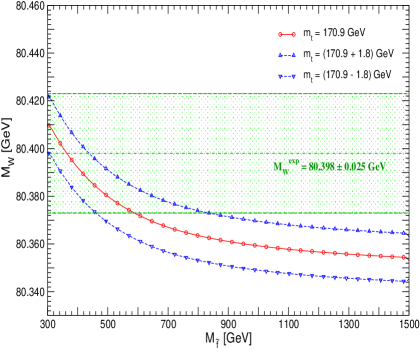
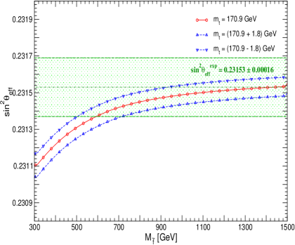
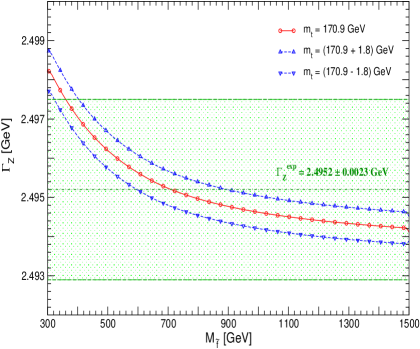
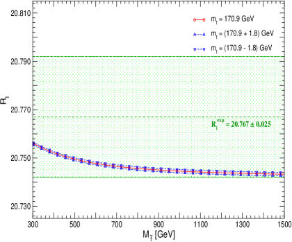
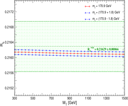
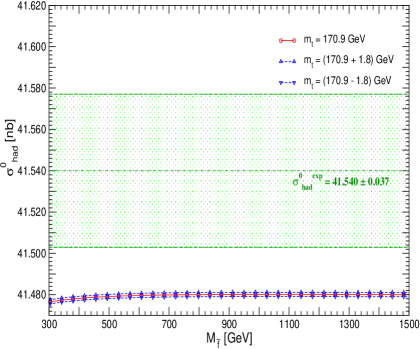
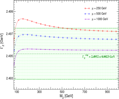
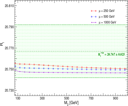
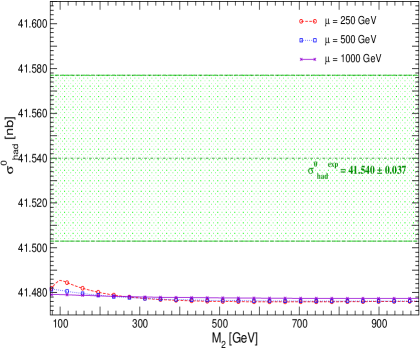
In Fig. 3 we show the prediction for the EWPO for real parameters as a function of $M_{\tilde{f}}$ and indicate how this prediction changes if the top-quark mass is varied within its experimental $1\sigma$ interval, $m_{t}=(170.9\pm 1.8)\,\,\mathrm{GeV}$ [79]. The other parameters are $A_{t,b,\tau}=2\,M_{\tilde{f}}$, $\mu=M_{A}=m_{\tilde{g}}=M_{2}=300\,\,\mathrm{GeV}$ and $\tan\beta=10$. The result is compared with the current experimental values, see Tab. 1. It can be seen in Fig. 3 that only $M_{W}$, $\sin^{2}\theta_{\mathrm{eff}}$ and $\Gamma_{Z}$ exhibit a pronounced sensitivity to $M_{\tilde{f}}$. While $M_{W}$ shows a mild preference for light $M_{\tilde{f}}$, $\sin^{2}\theta_{\mathrm{eff}}$ is in better agreement with the experimental value for large $M_{\tilde{f}}$. In interpreting the latter result it should be noted that the world-average on $\sin^{2}\theta_{\mathrm{eff}}$ involves independent measurements that differ from each other by more than three standard deviations [1]. An experimental resolution of this issue will most likely require an ILC with a GigaZ option. The prediction for $\Gamma_{Z}$ lies within its observed $1\sigma$ error for most of the parameter space. The dependence of $R_{l}$, $R_{b}$, and $\sigma^{0}_{\rm had}$ on $M_{\tilde{f}}$ is nearly flat, where the first two observables are within the $1\sigma$ band, and the latter is slightly below. The impact of varying $m_{t}$ within its experimental error is non-negligible only for $M_{W}$, $\sin^{2}\theta_{\mathrm{eff}}$, and $\Gamma_{Z}$. It results in the following shifts

$$\delta M_{W}^{{\rm para},m_{t}}=11\,\,\mathrm{MeV},$$ (74)

$$\delta m_{t}^{\rm exp}=1.8\,\,\mathrm{GeV}~{}\textup{\cite[cite]{[\@@bibref{}{mt1709}{}{}]}}\quad\Rightarrow\quad \delta\sin^{2}\theta_{\mathrm{eff}}^{{\rm para},m_{t}}=5.4\times 10^{-5},$$ (75)

$$\delta\Gamma_{Z}^{{\rm para},m_{t}}=0.43\,\,\mathrm{MeV}.$$ (76)

Similarly we have analysed the impact of a shift in $\Delta\alpha_{\rm had}^{(5)}$,

$$\delta M_{W}^{{\rm para},\Delta\alpha_{\rm had}^{(5)}}=6.3\,\,\mathrm{MeV},$$ (77)

$$\delta(\Delta\alpha_{\rm had}^{(5)})=3.5\times 10^{-4}\textup{\cite[cite]{[\@@bibref{}{LEPEWWG,DeltaAlfaMartin,Burkhardt:2005se}{}{}]}}\quad\Rightarrow\quad \delta\sin^{2}\theta_{\mathrm{eff}}^{{\rm para},\Delta\alpha_{\rm had}^{(5)}}=12\times 10^{-5},$$ (78)

$$\delta\Gamma_{Z}^{{\rm para},\Delta\alpha_{\rm had}^{(5)}}=0.32\,\,\mathrm{MeV}.$$ (79)

It should be noted that the parametric uncertainty in $\sin^{2}\theta_{\mathrm{eff}}$ induced by $\delta(\Delta\alpha_{\rm had}^{(5)})$ is of similar size as the current experimental uncertainty. A significant improvement of the uncertainty in $\Delta\alpha_{\rm had}^{(5)}$ is clearly very desirable in order to be able to fully exploit future progress in the experimental measurements of the EWPO as well as in their theoretical predictions, see also Sect. 6.

Figure 3: Prediction for $M_{W}$, $\sin^{2}\theta_{\mathrm{eff}}$, $\Gamma_{Z}$, $R_{l}$, $R_{b}$ and $\sigma_{\textup{had}}^{0}$ as function of the common sfermion mass scale $M_{\tilde{f}}$ for $m_{t}=(170.9\pm 1.8)\,\,\mathrm{GeV}$. The SUSY parameters are $\tan\beta=10$, $A_{\tau}=A_{t}=A_{b}=2M_{\tilde{f}}$, $M_{A}=\mu=m_{\tilde{g}}=M_{2}=300\,\,\mathrm{GeV}$.

5.1.2 Dependence on $\mu$ and $M_{2}$

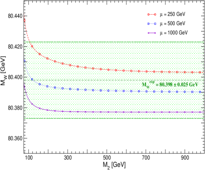
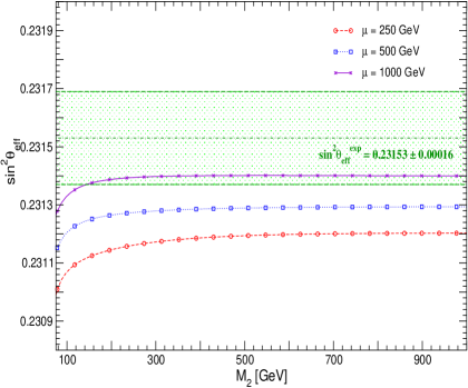
The variation of the EWPO with the parameters from the chargino/neutralino sector is investigated in Fig. 4. We show the prediction for the six EWPO as a function of $M_{2}$ for $\mu=250,500,$ $1000\,\,\mathrm{GeV}$ (and $M_{1}$ is chosen according to the GUT relation). The other parameters are set to $M_{\tilde{f}}=300\,\,\mathrm{GeV}$, $A_{t,b,\tau}=2M_{\tilde{f}}$, $M_{A}=1000\,\,\mathrm{GeV}$, $\tan\beta=10$ and $m_{\tilde{g}}=600\,\,\mathrm{GeV}$. As expected, also in this case the observables with the largest sensitivity to the variation of the SUSY parameters are $M_{W}$, $\sin^{2}\theta_{\mathrm{eff}}$ and $\Gamma_{Z}$. The impact of varying $M_{2}$ and $\mu$ on the other three observables is negligible. The variation with $\mu$ results in shifts in $M_{W}$, $\sin^{2}\theta_{\mathrm{eff}}$ and $\Gamma_{Z}$ at the $1\,\sigma$ level. A sizable variation with $M_{2}$ can only be observed for $M_{2}\;\raisebox{-3.00003pt}{$\stackrel{{\scriptstyle\displaystyle<}}{{\sim}}$}\;200\,\,\mathrm{GeV}$ for this set of parameters. While $M_{W}$ ($\sin^{2}\theta_{\mathrm{eff}}$) shows a monotonous decrease (increase) by $\sim 1\sigma$ with $M_{2}$, $\Gamma_{Z}$ exhibits a strong increase up to $M_{2}\;\raisebox{-3.00003pt}{$\stackrel{{\scriptstyle\displaystyle<}}{{\sim}}$}\;150\,\,\mathrm{GeV}$ and then slowly decreases for further increasing $M_{2}$. Good agreement between the $\Gamma_{Z}$ prediction and the experimental value is found for small $M_{2}$, see also Sect. 5.6.

Figure 4: Prediction for $M_{W}$, $\sin^{2}\theta_{\mathrm{eff}}$, $\Gamma_{Z}$, $R_{l}$, $R_{b}$ and $\sigma_{\textup{had}}^{0}$ as function of $M_{2}$ for $\mu=250,500,1000\,\,\mathrm{GeV}$. The remaining SUSY parameters are $\tan\beta=10$, $M_{\tilde{f}}=300\,\,\mathrm{GeV}$, $A_{\tau}=A_{t}=A_{b}=2M_{\tilde{f}}$, $m_{\tilde{g}}=600\,\,\mathrm{GeV}$, $M_{A}=1000\,\,\mathrm{GeV}$.

5.1.3 Dependence on complex phases

For the analysis of the dependence of the complex phases we focus on the three EWPO that show the strongest variation with the SUSY parameters, $M_{W}$, $\sin^{2}\theta_{\mathrm{eff}}$ and $\Gamma_{Z}$, see the two previous subsections. Since the dependence on the sfermion mass parameters is much stronger than on the chargino/higgsino parameters we only investigate the dependence on the phases of $A_{t}$ and $A_{b}$. As for $\Delta r/M_{W}$ [30] we find that the effective one-loop couplings $g^{f}_{\{V,A\},(1)}$ depend only on the absolute values $|X_{t}|$, $|X_{b}|$ of the off-diagonal entries in the $\tilde{t}$ and $\tilde{b}$ mass matrices, where $X_{t}=A_{t}-\mu/\tan\beta$, $X_{b}=A_{b}-\mu\,\tan\beta$. Thus, the phases of $\mu$, $A_{t}$ and $A_{b}$ enter only in the combinations $(\phi_{A_{t,b}}+\phi_{\mu})$, giving rise to modifications of the squark masses and mixing angles. It furthermore follows that the impact of $\phi_{A_{t}}$ ($\phi_{A_{b}}$) on the sfermion masses (see eq. (6)) is stronger for low (high) $\tan\beta$.

In Fig. 5 we show the three EWPO as a function of $\phi_{A_{t}}$ (with $\phi_{\mu}=\phi_{A_{b}}=0$, left plots) and $\phi_{A_{b}}$ (with $\phi_{\mu}=\phi_{A_{t}}=0$, right plots) for different values of $\tan\beta$ (varied from $\tan\beta=5$ to $\tan\beta=45$). The other parameters are set to $M_{\tilde{f}}=M_{H^{\pm}}=M_{2}=m_{\tilde{g}}=500\,\,\mathrm{GeV}$, $|A_{t,b,\tau}|=|\mu|=1000\,\,\mathrm{GeV}$, $\phi_{A_{\tau}}=\phi_{M_{1}}=\phi_{\tilde{g}}=0$. As expected, the dependence of $M_{W}$, $\sin^{2}\theta_{\mathrm{eff}}$ and $\Gamma_{Z}$ on $\phi_{A_{t}}$ is most pronounced for small $\tan\beta$ (see left panel of Fig. 5). The variation of $\phi_{A_{t}}$ in this case gives rise to a shift in the three precision observables by $1$–$2\sigma$. The effect becomes smaller for increasing $\tan\beta$, up to $\tan\beta=15$. On the other hand, for high $\tan\beta$ the lighter $\tilde{b}$ mass becomes rather small for the parameters chosen in Fig. 5, reaching values as low as about $100\,\,\mathrm{GeV}$ for $\tan\beta=45$. This leads to a sizable shift of $\sim 1$–$2\sigma$ in the EWPO already for vanishing phases. The slight rise in the dependence on $\phi_{A_{t}}$ for $\tan\beta\geq 25$ is due to the overall enlarged SUSY contributions which occur for large $\tan\beta$ and the resulting low sbottom masses.

Figure 5: Prediction for $M_{W}$, $\sin^{2}\theta_{\mathrm{eff}}$, and $\Gamma_{Z}$ as function of the phase of the trilinear coupling $A_{t}$ (plots on the left hand side) and $A_{b}$ (plots on the right hand side). The other SUSY parameters are: $M_{\tilde{f}}=M_{H^{\pm}}=M_{2}=m_{\tilde{g}}=500\,\,\mathrm{GeV},A_{\tau}=A_{t}=A_{b}=\mu=1000\,\,\mathrm{GeV},\phi_{A_{\tau}}=\phi_{\mu}=\phi_{M_{1}}=\phi_{\tilde{g}}=0,\phi_{A_{b}}=0$ (plots on the left), $\phi_{A_{t}}=0$ (plots on the right).

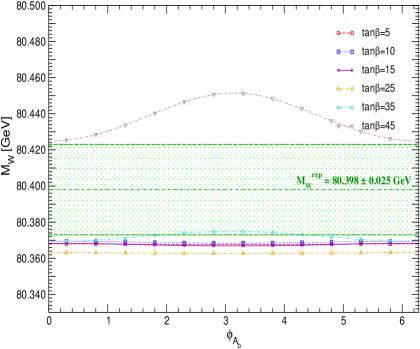
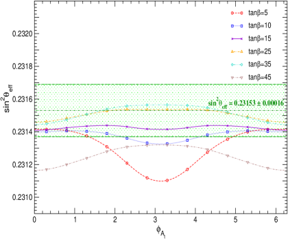
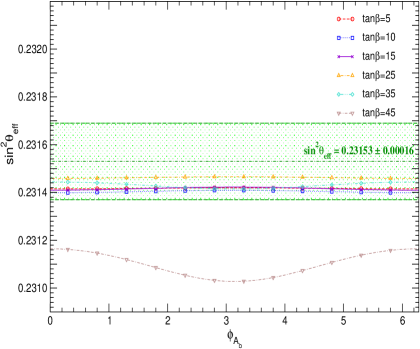
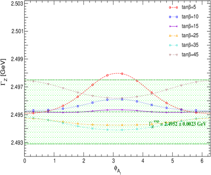
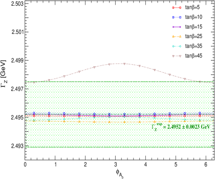
The dependence of the precision observables on $\phi_{A_{b}}$ (plots on the right-hand side of Fig. 5) is rather small, except for the highest $\tan\beta$ value shown in Fig. 5, $\tan\beta=45$. This is again related to the sizable correction induced by the lighter $\tilde{b}$ mass. In this scenario the variation of $\phi_{A_{b}}$ yields a shift in $M_{W}$, $\sin^{2}\theta_{\mathrm{eff}}$ and $\Gamma_{Z}$ at the $1\sigma$ level.

5.2 Impact of $Z\to\tilde{\chi}^{0}_{1}\tilde{\chi}^{0}_{1}$

As next step in our numerical analysis we investigate the impact of the decay $Z\to\tilde{\chi}^{0}_{1}\tilde{\chi}^{0}_{1}$ on the invisible $Z$ boson width, $\Gamma_{\textup{inv}}$. A sizable $Z\tilde{\chi}^{0}_{1}\tilde{\chi}^{0}_{1}$ coupling in combination with a light neutralino, $m_{\tilde{\chi}^{0}_{1}}\;\raisebox{-3.00003pt}{$\stackrel{{\scriptstyle\displaystyle<}}{{\sim}}$}\;M_{Z}/2$, results in an additional contribution to the invisible width of the $Z$ boson, in addition to the SM decays into neutrinos. Since the experimental result for the invisible width of the $Z$ boson is somewhat below the SM prediction [1], additional contributions from new physics are tightly constrained. It is of interest in how far the possibility of a light neutralino is affected by the precision measurement of the invisible width of the $Z$ boson.

The mass of the lightest neutralino is determined by $M_{1}$, $M_{2}$ and $\mu$, see eq. (10) (here we assume all parameters to be real). If $M_{1}$ or $M_{2}$ or $\mu$ is much smaller than the other two, the lightest neutralino is mostly a bino, zino, or higgsino, respectively. Its mass is to a large extent determined by this smallest mass value. If the condition

$$M_{1}=M_{1}^{(0)}\equiv 2M_{Z}^{2}s_{\mathrm{w}}^{2}\frac{\tan\beta}{(1+\tan^{2}\beta\hskip 2.84526pt)}\frac{M_{2}}{(\mu M_{2}-2M_{Z}^{2}\tan\beta/(1+\tan^{2}\beta\hskip 2.84526pt)c_{\mathrm{w}}^{2})}$$ (80)

was exactly fulfilled, the lightest neutralino, $\tilde{\chi}^{0}_{1}$, would be massless and almost entirely bino-like.

Figure 6: The invisible $Z$ boson width $\Gamma_{\textup{inv}}$ in- and excluding the process $Z\to\tilde{\chi}^{0}_{1}\tilde{\chi}^{0}_{1}$ is shown as a function of $M_{1}$ (left) and $m_{\tilde{\chi}^{0}_{1}}$ (right). The SUSY parameters are chosen to be: $M_{\tilde{f}}=250\,\,\mathrm{GeV},A_{\tau}=A_{t}=A_{b}=\mu=m_{\tilde{g}}=500\,\,\mathrm{GeV},M_{A}=500\,\,\mathrm{GeV},M_{2}=200\,\,\mathrm{GeV}$. A light, almost entirely bino-like, $\tilde{\chi}^{0}_{1}$ is obtained by varying $M_{1}$ around the value $M_{1}^{(0)}$ defined in eq. (80) within the range of $-100$ to $+100\,\,\mathrm{GeV}$.

Figure 7: The invisible $Z$ boson width $\Gamma_{\textup{inv}}$ in- and excluding the process $Z\to\tilde{\chi}^{0}_{1}\tilde{\chi}^{0}_{1}$ is shown as a function of $M_{1}$ (left) and $m_{\tilde{\chi}^{0}_{1}}$ (right). The SUSY parameters are chosen as follows: $M_{\tilde{f}}=A_{\tau}=A_{t}=A_{b}=M_{A}=m_{\tilde{g}}=600\,\,\mathrm{GeV},\mu=125\,\,\mathrm{GeV},M_{2}=200\,\,\mathrm{GeV}$, $M_{1}=-100\dots 100\,\,\mathrm{GeV}$.

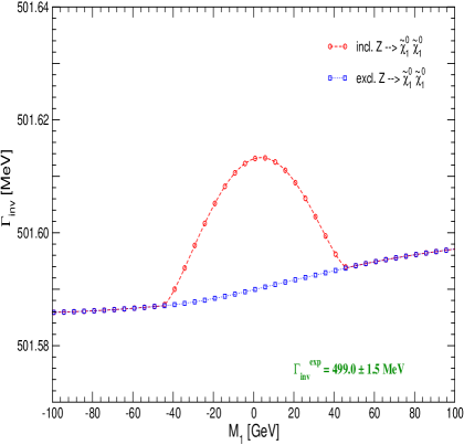
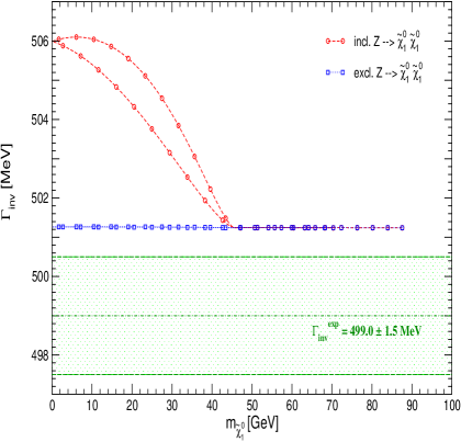
In Fig. 6 we analyse a scenario with a light neutralino (see also the discussion in Ref. [94]). We do this by varying $M_{1}$ around the value $M_{1}^{(0)}$ defined in eq. (80), i.e.

$$M_{1}=M_{1}^{(0)}+\Delta M,$$ (81)

where we let $\Delta M$ run from $-100$ to $+100\,\,\mathrm{GeV}$. The other parameters in Fig. 6 are $M_{\tilde{f}}=250\,\,\mathrm{GeV}$, $A_{t,b,\tau}=\mu=m_{\tilde{g}}=M_{A}=500\,\,\mathrm{GeV}$, $M_{2}=200\,\,\mathrm{GeV}$, $\tan\beta=10$. In the left (right) plot of Fig. 6 the results for $\Gamma_{\textup{inv}}$ are shown as a function of $M_{1}$ ($m_{\tilde{\chi}^{0}_{1}}$). The curves in the plot on the right hand side of Fig. 6 consist of two branches for a given value of $m_{\tilde{\chi}^{0}_{1}}$. This is a consequence of the fact that different values of $M_{1}$ in general lead to different values of $\Gamma_{\textup{inv}}$ although the value of $m_{\tilde{\chi}^{0}_{1}}$ may be the same. Comparing with the plot on the left one can see that the upper branch corresponds to $M_{1}\;\raisebox{-3.00003pt}{$\stackrel{{\scriptstyle\displaystyle>}}{{\sim}}$}\;0$, the lower branch to $M_{1}\;\raisebox{-3.00003pt}{$\stackrel{{\scriptstyle\displaystyle<}}{{\sim}}$}\;0$. The coupling of a nearly pure bino to $Z$ bosons is very weak, resulting in a visible, but negligible effect on $\Gamma_{\textup{inv}}$. The entire range of $\Gamma_{\textup{inv}}$ shown in Fig. 6 is outside its $1\sigma$ error. As mentioned above, this is a consequence of the well-known fact that the measured value of the invisible $Z$ width is below the SM prediction [1]. As the predictions including and excluding the process $Z\to\tilde{\chi}^{0}_{1}\tilde{\chi}^{0}_{1}$ differ at most by $\sim 0.02\,\,\mathrm{MeV}$, compared to an experimental range of $\Gamma_{\textup{inv}}^{\textup{exp}}=499.0\pm 1.5\,\,\mathrm{MeV}$, the inclusion of the decay into neutralinos $\tilde{\chi}^{0}_{1}$ clearly does not give rise to additional constraints on $M_{1}$ or the mass of the lightest neutralino $m_{\tilde{\chi}^{0}_{1}}$ in this scenario.

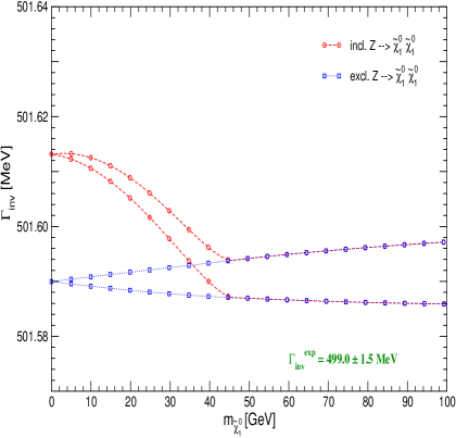
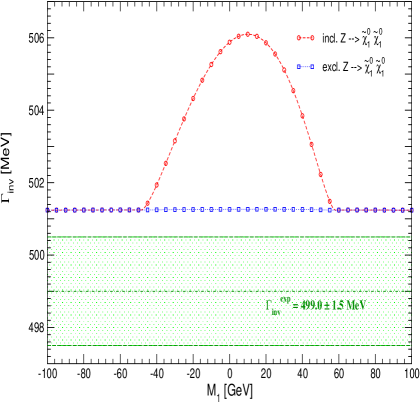
A different scenario with $\mu\sim M_{1}$, but $M_{1}\;\raisebox{-3.00003pt}{$\stackrel{{\scriptstyle\displaystyle<}}{{\sim}}$}\;\frac{1}{2}M_{2}$ (in coarse agreement with the GUT relation) is analysed in Fig. 7. The parameters are set to $M_{\tilde{f}}=A_{t,b,\tau}=M_{A}=m_{\tilde{g}}=600\,\,\mathrm{GeV}$, $\mu=125\,\,\mathrm{GeV}$, $M_{2}=200\,\,\mathrm{GeV}$, $\tan\beta=10$, and $M_{1}$ is varied from $-100\,\,\mathrm{GeV}$ to $+100\,\,\mathrm{GeV}$. In this scenario the lightest neutralino can have a sizable higgsino component. In the left (right) plot of Fig. 7 the results for $\Gamma_{\textup{inv}}$ are shown as a function of $M_{1}$ ($m_{\tilde{\chi}^{0}_{1}}$). The lower branches in Fig. 7 (plot on the right) again correspond to $M_{1}\;\raisebox{-3.00003pt}{$\stackrel{{\scriptstyle\displaystyle<}}{{\sim}}$}\;0$, the upper branches to $M_{1}\;\raisebox{-3.00003pt}{$\stackrel{{\scriptstyle\displaystyle>}}{{\sim}}$}\;0$. For values $m_{\tilde{\chi}^{0}_{1}}\;\raisebox{-3.00003pt}{$\stackrel{{\scriptstyle\displaystyle<}}{{\sim}}$}\;M_{Z}/2$ the $\Gamma_{\tilde{\chi}^{0}_{1}}$ contribution to $\Gamma_{\textup{inv}}$ becomes sizable. In this case the deviation between the MSSM prediction for the invisible $Z$ width and the measured value, which is slightly above $1\sigma$ if the decay into neutralinos is not open, raises above the $2\sigma$ level for $|M_{1}|\;\raisebox{-3.00003pt}{$\stackrel{{\scriptstyle\displaystyle<}}{{\sim}}$}\;35\,\,\mathrm{GeV}$ or $m_{\tilde{\chi}^{0}_{1}}\;\raisebox{-3.00003pt}{$\stackrel{{\scriptstyle\displaystyle<}}{{\sim}}$}\;35\,\,\mathrm{GeV}$.

As a consequence, if the SUSY parameters are such that $\tilde{\chi}^{0}_{1}$ has a sizable coupling to the $Z$ boson (e.g. $M_{2}>M_{1}\gg\mu$), the theoretical prediction for $\Gamma_{\textup{inv}}$ can easily exceed the experimental central value by several standard deviations (provided that $m_{\tilde{\chi}^{0}_{1}}<M_{Z}/2$). In such a scenario the contribution to the invisible width arising from $\Gamma_{\tilde{\chi}^{0}_{1}}$ yields interesting constraints on the parameters $\mu$, $M_{1}$, and $M_{2}$.

5.3 The SPS benchmark scenarios

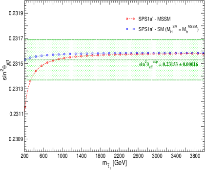
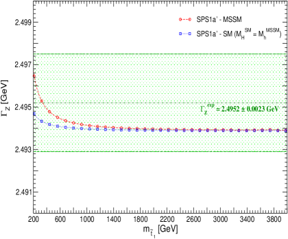
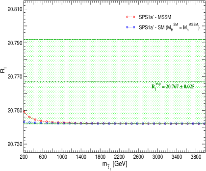
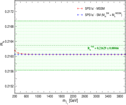
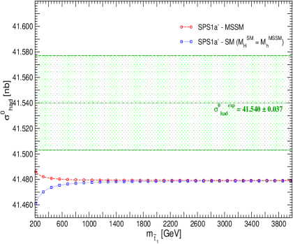
In this section we analyse the six EWPO $M_{W}$, $\sin^{2}\theta_{\mathrm{eff}}$, $\Gamma_{Z}$, $R_{l}$, $R_{b}$, and $\sigma^{0}_{\rm had}$ in the SPS 1a^′, SPS 1b and SPS 5 benchmark scenarios [32, 95]. Our analysis extends the results of Ref. [30] to the $Z$ pole observables. In order to analyse the dependence of the EWPO on the scale of supersymmetry we scale for each SPS point all SUSY parameters carrying mass dimension by a common factor, i.e. $M_{A}=(\textup{scalefactor})\times M_{A}^{\textup{SPS}}$, $M_{{\tilde{F}},{\tilde{F}^{\prime}}}=(\textup{scalefactor})\times M_{{\tilde{F}},{\tilde{F}^{\prime}}}^{\textup{SPS}}$, $A_{t,b,\tau}=(\textup{scalefactor})\times A_{t,b,\tau}^{\textup{SPS}}$, $\mu=(\textup{scalefactor})\times\mu^{\textup{SPS}}$, $M_{1,2,3}=(\textup{scalefactor})\times M_{1,2,3}^{\textup{SPS}}$. In Fig. 8 we show $M_{W}$, $\sin^{2}\theta_{\mathrm{eff}}$, $\Gamma_{Z}$, $R_{l}$, $R_{b}$, and $\sigma^{0}_{\rm had}$ as a function of the lighter $\tilde{t}$ mass, $m_{\tilde{t}_{1}}$, in the three SPS scenarios. As before, only $M_{W}$, $\sin^{2}\theta_{\mathrm{eff}}$ and $\Gamma_{Z}$ show a sizable variation with $m_{\tilde{t}_{1}}$ (i.e., the scalefactor). For all the EWPO the (loop-induced) variation between the three SPS scenarios is relatively small. $M_{W}$ shows best agreement with the experimental results for low $m_{\tilde{t}_{1}}$. $\sin^{2}\theta_{\mathrm{eff}}$ lies in the $\pm 1\,\sigma$ range for $m_{\tilde{t}_{1}}\;\raisebox{-3.00003pt}{$\stackrel{{\scriptstyle\displaystyle>}}{{\sim}}$}\;400\,\,\mathrm{GeV}$. $\Gamma_{Z}$ shows a variation with $m_{\tilde{t}_{1}}$ of $\sim 1\,\sigma$ around the experimental value.

Figure 8: Predictions for $M_{W}$, $\sin^{2}\theta_{\mathrm{eff}}$, $\Gamma_{Z}$, $R_{l}$, $R_{b}$ and $\sigma_{\textup{had}}^{0}$ within the SPS1a^′, SPS1b and SPS5 scenarios. The observables are shown as a function of $m_{\tilde{t}_{1}}$, the mass of the lighter of the two scalar top-quarks. The SPS parameters of mass dimension are varied with the scale of supersymmetry as described in the text.

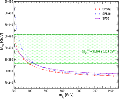
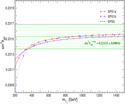
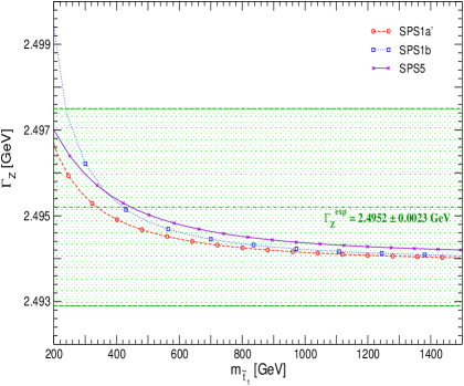
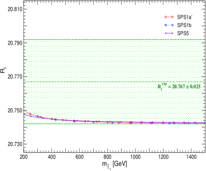
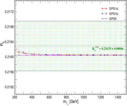
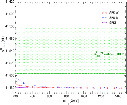
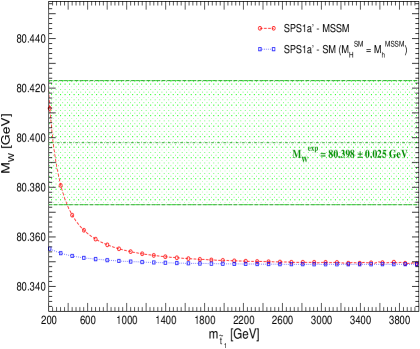
Fig. 9 shows for the example of the SPS 1a^′ scenario that, as expected, the MSSM predictions for the EWPO approach the corresponding predictions in the SM (for $M^{\textup{SM}}_{H}=M_{h}^{\rm MSSM}$) for large values of the SUSY mass scale. The predictions within the MSSM and the SM (for $M^{\textup{SM}}_{H}=M_{h}^{\rm MSSM}$) are shown as a function of $m_{\tilde{t}_{1}}$ (as before, all parameters carrying mass dimension are scaled by a common factor). The variation of the SM prediction with the SUSY scale is induced by the corresponding change in the light ${\cal CP}$-even Higgs-boson mass. The difference between the MSSM and the SM predictions becomes negligible for $m_{\tilde{t}_{1}}\;\raisebox{-3.00003pt}{$\stackrel{{\scriptstyle\displaystyle>}}{{\sim}}$}\;2000\,\,\mathrm{GeV}$ for $M_{W}$ and $\sin^{2}\theta_{\mathrm{eff}}$. For the other EWPO the decoupling of the supersymmetric contributions occurs for even lower values of $m_{\tilde{t}_{1}}$. For the hadronic peak cross section, $\sigma^{0}_{\rm had}$, the change with the SUSY scale in the MSSM and the SM prediction has opposite signs (on the other hand, for the individual factors entering $\sigma^{0}_{\rm had}$, see eq. (52), the dependence of the MSSM and SM predictions on the SUSY scale goes into the same direction). The fact that we recover the most up-to-date SM prediction for the EWPO in the decoupling limit is a consequence of the procedure described in Sect. 4.2.1 (see eq. (59)).

Figure 9: Predictions for $M_{W}$, $\sin^{2}\theta_{\mathrm{eff}}$, $\Gamma_{Z}$, $R_{l}$, $R_{b}$ and $\sigma_{\textup{had}}^{0}$ within the SPS1a^′ scenario in comparison with the SM result calculated for $M^{\textup{SM}}_{H}=M_{h}$. The observables are shown as a function of $m_{\tilde{t}_{1}}$, the mass of the lighter of the two scalar top-quarks. The SPS parameters of mass dimension are varied with the scale of supersymmetry as described in the text.

5.4 The CPX benchmark scenario

In this section we analyse the prediction of the EWPO in the CPX scenario. This scenario is defined as [35]

$$M_{\tilde{f}}=500\,\,\mathrm{GeV},|A_{t}|=1000\,\,\mathrm{GeV},A_{t}=A_{b}=A_{\tau}$$

$$M_{2}=200\,\,\mathrm{GeV},|m_{\tilde{g}}|=1000\,\,\mathrm{GeV},\mu=2000\,\,\mathrm{GeV}$$ (82)

$$\phi_{A_{t,b,\tau}}=\phi_{\tilde{g}}=\pi/2~{},$$

with the aim to indicate the possible size of ${\cal CP}$-violating effects.

The LEP Higgs searches have been interpreted within the CPX scenario [96]. A parameter region for intermediate $\tan\beta$ and and light $M_{h_{1}}$ could not be excluded at the 95% C.L., so that no lower limit on the mass of the lightest Higgs boson could be set. The reason for the appearance of these “CPX holes” is a strong suppression of the coupling of the lightest Higgs boson to gauge bosons, while the second lightest Higgs boson (also having a somewhat reduced coupling to gauge bosons), which may also be within the kinematic reach of LEP, decays predominantly into the lightest Higgs boson. The latter leads to a rather difficult topology of the final state.

As a consequence of its strongly suppressed coupling to gauge bosons, the impact of the contributions of a light Higgs boson associated with the “CPX holes” on the EWPO is expected to be rather small. In Fig. 10 we investigate whether the current measurements of the EWPO, see Tab. 1, allow to put constraints on the parameter space of the “CPX holes”. The consistent inclusion of the loop-corrected Higgs boson masses and couplings is crucial for this analysis.

Figure 10: Predictions for $M_{W}$, $\sin^{2}\theta_{\mathrm{eff}}$, $\Gamma_{Z}$, $R_{l}$, $R_{b}$ and $\sigma_{\textup{had}}^{0}$ within the CPX benchmark scenario for $\tan\beta=3\dots 13$ as a function of $M_{H^{\pm}}$, the mass of the charged Higgs boson. In the last row the masses $M_{h_{1}}$, $M_{h_{2}}$, $M_{h_{3}}$ of the three neutral Higgs bosons in the ${\cal CP}$-violating case are shown.

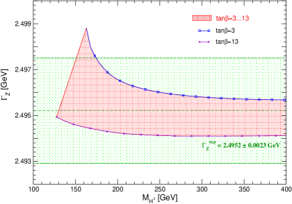
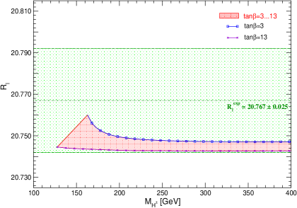
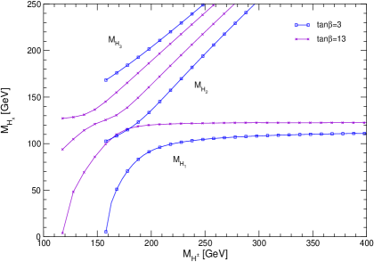
In Fig. 10 we show the predictions of the six EWPO as a band for the range $\tan\beta=3$–$13$, where the blue curves (boxes) correspond to $\tan\beta=3$, the purple curves (crosses) to $\tan\beta=13$. The band is to the left cut off for the lowest physically allowed values of $M_{H^{\pm}}$. (For illustrative purposes we also show the values of the three neutral Higgs boson masses in the lowest plot of Fig. 10 as obtained with FeynHiggs [43, 44, 40].) The regions unexcluded by the LEP Higgs searches (starting at $\tan\beta\approx 3.6$) are indicated by a light blue shading for the two observables $M_{W}$ and $\sin^{2}\theta_{\mathrm{eff}}$ (for simplicity, we have omitted them for the other observables). As explained above, our one-loop result contains the full complex phase dependence, whereas at the two-loop level we use the approximation formula given in eq. (60). While this method works for $\tan\beta=13$, for $\tan\beta=3$ the value for $\phi=\pi$ (see eq. (60)) cannot be evaluated since (at least) one of the squark mass squares turns negative. Therefore for $\tan\beta=3$ we use $O(\phi)=O^{\rm 1L}(\phi)+(O^{\rm full}(0)-O^{\rm 1L}(0))$, $O=M_{W}$, $\sin^{2}\theta_{\mathrm{eff}}$, $\Gamma_{Z}$, $R_{l}$, $R_{b}$, $\sigma^{0}_{\rm had}$. This results in a higher theoretical uncertainty of the prediction for the $\tan\beta=3$ border shown in Fig. 10, which should be kept in mind for the interpretation of the figure.

Fig. 10 shows that the predictions for the EWPO in this parameter region of the CPX scenario are in general in good agreement with the experimental results. Only for low $\tan\beta$ (i.e., values close to the boundary of the region indicated by the contour with $\tan\beta=3$) and small $M_{H^{\pm}}$ sizable deviations can be observed, most notably for $\sin^{2}\theta_{\mathrm{eff}}$. On the other hand, the parameter regions corresponding to the “CPX holes” show only small deviations from the EWPO. Most of the corresponding regions are even within the 1 $\sigma$ intervals of the experimental values of $M_{W}$ and $\sin^{2}\theta_{\mathrm{eff}}$. Thus, more precise EWPO measurements combined with improved theoretical predictions (and correspondingly smaller intrinsic uncertainties in the EWPO calculations) would be needed to reach the sensitivity for probing the “CPX hole” regions via their effects on EWPO.

5.5 Scenario where no SUSY particles are observed at the LHC

It is interesting to investigate whether the high accuracy achievable at the GigaZ option of the ILC would provide sensitivity to indirect effects of SUSY particles even in a scenario where the (strongly interacting) superpartners are so heavy that they escape detection at the LHC.

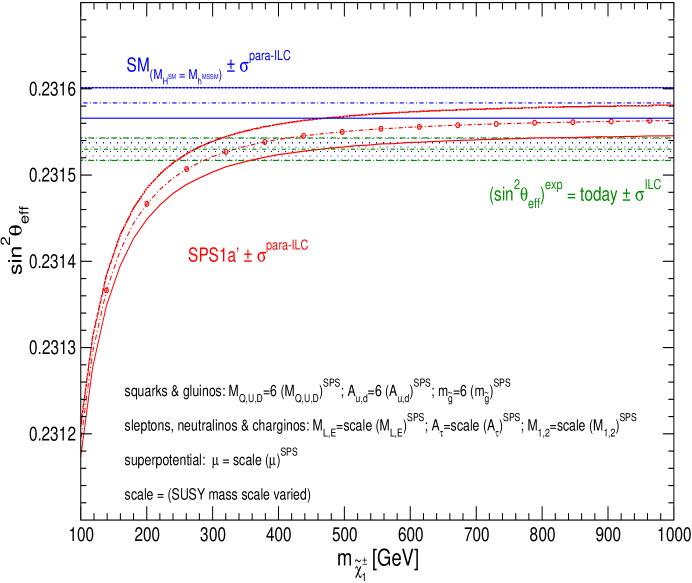
We consider in this context a scenario with very heavy squarks and a very heavy gluino. It is based on SPS 1a^′, but the squark and gluino mass parameters are fixed to 6 times their SPS 1a^′ values. The other masses are scaled with a common scale factor as described in Sect. 5.3, except $M_{A}$ which we keep fixed at its SPS 1a^′ value. In this scenario the strongly interacting particles are too heavy to be detected at the LHC, while, depending on the scale-factor, some colour-neutral particles may be in the ILC reach (the reach for the direct production of colour-neutral particles at the LHC will be rather limited [97]). In Fig. 11 we show the prediction for $\sin^{2}\theta_{\mathrm{eff}}$ in this SPS 1a^′ inspired scenario as a function of the lighter chargino mass, $m_{\tilde{\chi}^{\pm}_{1}}$. The prediction includes the parametric uncertainty, $\sigma^{\rm para-ILC}$, induced by the ILC measurement of $m_{t}$, $\delta m_{t}=100\,\,\mathrm{MeV}$ [98, 99], and the numerically more relevant prospective future uncertainty on $\Delta\alpha^{(5)}_{\textup{had}}$, $\delta(\Delta\alpha^{(5)}_{\textup{had}})=5\times 10^{-5}$ [100]. The MSSM prediction for $\sin^{2}\theta_{\mathrm{eff}}$ is compared with the experimental resolution with GigaZ precision, $\sigma^{\rm ILC}=0.000013$, using for simplicity the current experimental central value. The SM prediction (with $M^{\textup{SM}}_{H}=M_{h}^{\rm MSSM}$) is also shown, applying again the parametric uncertainty $\sigma^{\rm para-ILC}$.

Despite the fact that no coloured SUSY particles would be observed at the LHC in this scenario, the ILC with its high-precision measurement of $\sin^{2}\theta_{\mathrm{eff}}$ in the GigaZ mode could resolve indirect effects of SUSY up to $m_{\tilde{\chi}^{\pm}_{1}}\;\raisebox{-3.00003pt}{$\stackrel{{\scriptstyle\displaystyle<}}{{\sim}}$}\;500\,\,\mathrm{GeV}$. This means that the high-precision measurements at the ILC with GigaZ option could be sensitive to indirect effects of SUSY even in a scenario where SUSY particles have neither been directly detected at the LHC nor the first phase of the ILC with a centre of mass energy of up to $500\,\,\mathrm{GeV}$.

Figure 11: Theoretical prediction for $\sin^{2}\theta_{\mathrm{eff}}$ in the SM and the MSSM (including prospective parametric theoretical uncertainties) compared to the experimental precision at the ILC with GigaZ option. An SPS 1a^′ inspired scenario is used, where the squark and gluino mass parameters are fixed to 6 times their SPS 1a^′ values. The other mass parameters are varied with a common scalefactor, see Sect. 5.3.

5.6 Heavy scalar masses

The scenario discussed in the previous section is characterised by rather heavy scalar quarks (and a heavy gluino). Other scenarios with heavy scalar masses that found attention in recent years are the so-called “split SUSY” scenario [33] and the “focus point region” [34] of the CMSSM. For completeness, we also briefly discuss the sensitivity of the EWPO to these scenarios.

In the split SUSY scenario the fermionic masses (i.e. the chargino, neutralino, and gluino masses) are relatively light and retain their GUT-induced hierarchy, resulting in a heavier gluino and lighter charginos and neutralinos. The scalar mass parameters, on the other hand, are set to very large values, larger than $10^{6}$–$10^{9}\,\,\mathrm{GeV}$, i.e., they decouple from the predictions of the EWPO. Consequently, only a small deviation in the EWPO prediction from the SM limit is to be expected in this scenario. We focus here on the two most sensitive EWPO, $M_{W}$ and $\sin^{2}\theta_{\mathrm{eff}}$ (the results given for $M_{W}$ are an update of Ref. [30]).

Figure 12: $\delta M_{W}=(M_{W}^{\textup{MSSM}}-M_{W}^{\textup{SM}})$ (upper plot) and $\delta\sin^{2}\theta_{\mathrm{eff}}=(\sin^{2}\theta_{\mathrm{eff}}^{\textup{MSSM}}-\sin^{2}\theta_{\mathrm{eff}}^{\textup{SM}})$ (lower plot) in a split SUSY scenario. The SUSY parameters are $M_{\tilde{f}}=5000\,\,\mathrm{GeV},M_{A}=2500\,\,\mathrm{GeV},\tan\beta=10,A_{\tau}=A_{t}=A_{b}=2M_{\tilde{f}},m_{\tilde{g}}=500\,\,\mathrm{GeV}$. Contour lines are drawn for $\delta M_{W}=\big{\{}30\,\,\mathrm{MeV}$, $\sigma^{\textup{LHC}}=15\,\,\mathrm{MeV}$, $\sigma^{\textup{ILC}}=7\,\,\mathrm{MeV}$, $3\,\,\mathrm{MeV}$, $2\,\,\mathrm{MeV}\big{\}}$ and $\delta\sin^{2}\theta_{\mathrm{eff}}=\big{\{}30\times 10^{-5}$, $15\times 10^{-5}$, $3\sigma^{\textup{ILC}}=3.9\times 10^{-5}$, $2\sigma^{\textup{ILC}}=2.6\times 10^{-5}$, $\sigma^{\textup{ILC}}=1.3\times 10^{-5}\big{\}}$.

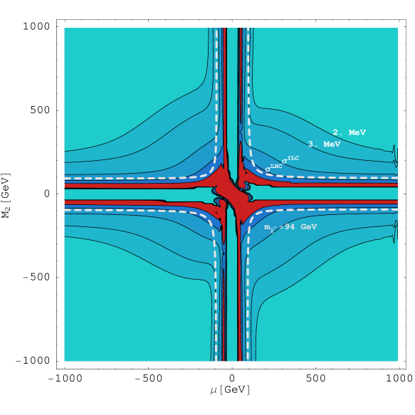
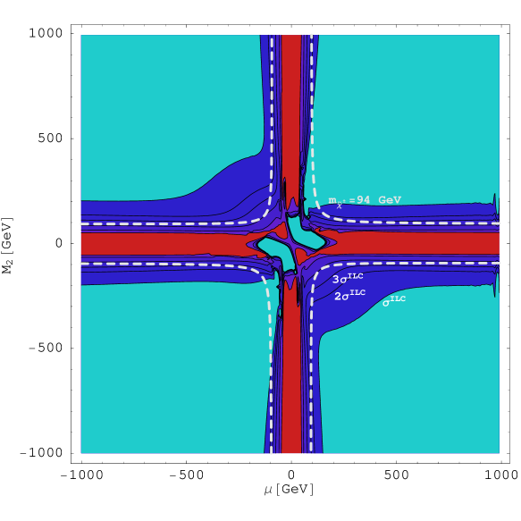
In Fig. 12 we show in a split SUSY scenario the SUSY contribution, i.e., the difference between the SUSY result and the corresponding SM result, to $M_{W}$ (upper plot) and to $\sin^{2}\theta_{\mathrm{eff}}$ (lower plot). This is done by choosing a large value for $M_{\tilde{f}}$ and subtracting the SM result with $M^{\textup{SM}}_{H}=M_{h}^{\rm MSSM}$ from the result obtained in the MSSM. We have chosen $M_{\tilde{f}}=5\,\,\mathrm{TeV}$ and $M_{A}=2.5\,\,\mathrm{TeV}$. Choosing even higher values for the scalar mass parameters would only lead to negligible shifts as compared to the results shown Fig. 12. The results are displayed in Fig. 12 in the $\mu$–$M_{2}$ plane for $\tan\beta=10$. The gluino mass has been fixed to $m_{\tilde{g}}=500\,\,\mathrm{GeV}$ (the results are insensitive to this choice). The results are given in terms of contour lines representing the different collider precisions, see Tab. 1. The region excluded by chargino searches at LEP [58] is inside the dashed white lines. As can be seen in the figure, deviations from the SM prediction of more than $30\,\,\mathrm{MeV}$ in $M_{W}$ and $3\times 10^{-4}$ in $\sin^{2}\theta_{\mathrm{eff}}$ occur only in those experimentally excluded areas. The parameter regions leading to a shift as large as the GigaZ precisions in $M_{W}$ of $1\sigma^{\rm ILC}=7\,\,\mathrm{MeV}$ and in $\sin^{2}\theta_{\mathrm{eff}}$ of $1\sigma^{\rm ILC}=0.000013$ are significantly larger. In particular, a 1 $\sigma$ effect in $\sin^{2}\theta_{\mathrm{eff}}$ can occur for $|\mu|,|M_{2}|\;\raisebox{-3.00003pt}{$\stackrel{{\scriptstyle\displaystyle<}}{{\sim}}$}\;400\,\,\mathrm{GeV}$ (for negative $(\mu M_{2})$ only). (Similar results were obtained in Ref. [101], see also Ref. [102].)

Another scenario with heavy scalar masses is the focus point region [34] in the CMSSM (the CMSSM is characterised by a common scalar mass parameter, $m_{0}$, a common fermionic mass parameter, $m_{1/2}$, and a common trilinear coupling, $A_{0}$, at the GUT scale, supplemented by the low-scale parameter $\tan\beta$ and the sign of the parameter $\mu$). In the focus point region $m_{1/2}$ is relatively small, while $m_{0}$ is rather large, $m_{0}\sim\mbox{ few}\,\,\mathrm{TeV}$, and also $\tan\beta$ is relatively large, $\tan\beta\;\raisebox{-3.00003pt}{$\stackrel{{\scriptstyle\displaystyle>}}{{\sim}}$}\;40$. We have investigated (using the program ISAJET 7.71 [103]) the predictions for $M_{W}$, $\sin^{2}\theta_{\mathrm{eff}}$ and $\Gamma_{Z}$ in the focus point region. The results for $\sin^{2}\theta_{\mathrm{eff}}$ and $\Gamma_{Z}$ follow the pattern observed in Ref. [30], where $M_{W}$ had been analysed. The main contributions to the shifts in the EWPO arise from the chargino and neutralino sector (see Sect. 5.1.2) and only very small effects arise from the scalar fermion contributions. For $\tan\beta=50$, $\mu>0$, $m_{1/2}=250\,\,\mathrm{GeV}$, $m_{0}=1500\,\,\mathrm{GeV}$, $A_{0}=-250\,\,\mathrm{GeV}$, corresponding to a point with the currently lowest value of $m_{1/2}$ in the focus point region for which the dark matter density is allowed by WMAP and other cosmological data (see, for example, Ref. [9] for a more detailed discussion), we find an effect of the SUSY contribution of $6\times 10^{-5}$ in $\sin^{2}\theta_{\mathrm{eff}}$ and $1\,\,\mathrm{MeV}$ in $\Gamma_{Z}$. Thus, even for the low-$m_{1/2}$ region of the focus point scenario the GigaZ precision for $\sin^{2}\theta_{\mathrm{eff}}$ will be needed to gain sensitivity to indirect effects in the EWPO.

5.7 Higgs sector at higher orders

We next investigate the impact of higher-order contributions associated with the Higgs sector of the MSSM. As mentioned above, since the Higgs sector enters the EWPO only via loop corrections, in order to evaluate predictions for the EWPO at one-loop order it would formally be sufficient to treat the Higgs sector in leading order, i.e., at tree level. However, at the tree level the predicted value for the mass of the light ${\cal CP}$-even Higgs boson is so low that it is below the exclusion limit from the Higgs searches at LEP [96, 104]. As a consequence, treating the MSSM Higgs sector at tree level in the predictions for the EWPO would lead to artificially large contributions to the EWPO from the light MSSM Higgs boson. Therefore a consistent incorporation of higher-order contributions in the Higgs sector, as described in Sect. 2.3, is crucial in order to be able to use realistic mass values for the light MSSM Higgs boson and to take into account potentially large higher-order effects.

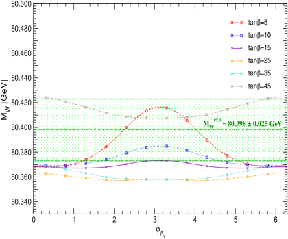
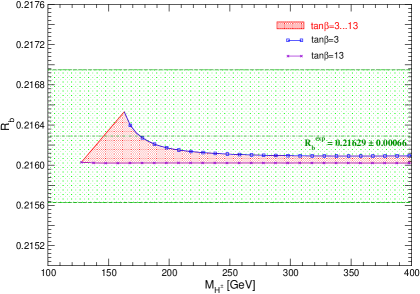
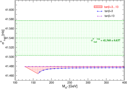
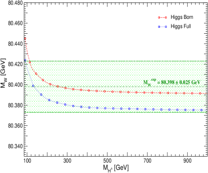
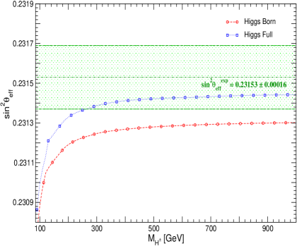
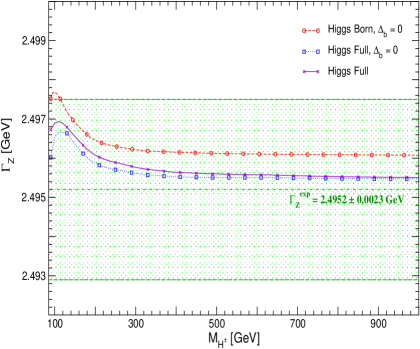
To analyse the numerical effects of higher-order contributions in the Higgs sector we study $M_{W}$, $\sin^{2}\theta_{\mathrm{eff}}$, $\Gamma_{Z},$ and $R_{b}$ for the MSSM parameter set $\tan\beta=50$, $M_{2}=300\,\,\mathrm{GeV}$, $m_{\tilde{g}}=600\,\,\mathrm{GeV}$, $M_{\tilde{f}}=300\,\,\mathrm{GeV}$, $\mu=300\,\,\mathrm{GeV}$, $|A_{t}|=|A_{b}|=|A_{\tau}|=2M_{\tilde{f}}$, $\phi_{A_{t}}=\pi/2$, $\phi_{A_{\tau}}=\phi_{A_{b}}=\phi_{\mu}=\phi_{M_{1}}=\phi_{\tilde{g}}=0$. $M_{H^{\pm}}$ is varied from $85\,\,\mathrm{GeV}$ to $1000\,\,\mathrm{GeV}$. A rather large value for $\tan\beta$ was chosen to further analyse a possible numerical impact of the resummation of leading $\tan\beta$ enhanced Higgs (s)bottom couplings in the process $Z\to b\bar{b}$, entering via $\Delta_{b}$, see eq. (16). Our results are shown in Fig. 13, where “Higgs Born” labels the numerical results where only Born-level Higgs masses and couplings were used. “Higgs Full” are the results which take into account the implementation described in Sect. 2.3, i.e., they account for loop-corrected Higgs masses and mixing angles, mixing of ${\cal CP}$ eigenstates in the presence of complex MSSM parameters, and $\tan\beta$ enhanced Higgs (s)bottom couplings, included via $\Delta_{b}$.

In the upper row of Fig. 13 we show the results for $M_{W}$ and $\sin^{2}\theta_{\mathrm{eff}}$. The impact of the higher-order corrections in the Higgs sector, corresponding to the difference between the two results shown in Fig. 13, amounts to a shift in $M_{W}$ and $\sin^{2}\theta_{\mathrm{eff}}$ of about $1\sigma$. Thus, this contribution, which is formally of two-loop order, has a sizable numerical impact and should be taken into account in order to arrive at a precise prediction for $M_{W}$ and $\sin^{2}\theta_{\mathrm{eff}}$. The lower row of Fig. 13 displays the results for $\Gamma_{Z}$ and $R_{b}$, where we also show the impact of the $\Delta_{b}$ corrections alone by comparing with the result where $\Delta_{b}=0$ (labeled as “Higgs Full, $\Delta_{b}=0$”). The numerical impact of the higher-order corrected Higgs boson sector on the observables $\Gamma_{Z}$ and $R_{b}$ relative to their current experimental errors is less pronounced as compared to $M_{W}$ and $\sin^{2}\theta_{\mathrm{eff}}$. Setting $\Delta_{b}=0$ yields only a relatively small shift from the full result. It should be kept in mind that $\Delta_{b}$, see eq. (16), approximates the leading contribution from the sbottom sector only for large SUSY mass scales. If the relevant particle masses are simultaneously small, $M_{\tilde{f}}\;\raisebox{-3.00003pt}{$\stackrel{{\scriptstyle\displaystyle<}}{{\sim}}$}\;m_{t}$, the theoretical uncertainties in the predictions of the EWPO can be slightly larger.

Figure 13: Predictions for $M_{W}$, $\sin^{2}\theta_{\mathrm{eff}}$, $\Gamma_{Z}$, and $R_{b}$ as a function of $M_{H^{\pm}}$. The MSSM parameters are $\tan\beta=50$, $M_{2}=300\,\,\mathrm{GeV}$, $m_{\tilde{g}}=600\,\,\mathrm{GeV}$, $M_{\tilde{f}}=300\,\,\mathrm{GeV}$, $\mu=300\,\,\mathrm{GeV}$, $|A_{t}|=|A_{b}|=|A_{\tau}|=2M_{\tilde{f}}$, $\phi_{A_{t}}=\pi/2$, $\phi_{A_{\tau}}=\phi_{A_{b}}=\phi_{\mu}=\phi_{\tilde{g}}=0$, $M_{H^{\pm}}=85\,\,\mathrm{GeV}\dots 1000\,\,\mathrm{GeV}$. “Higgs Born” labels the results calculated for Born-level Higgs sector parameters, while “Higgs Full” refers to the results calculated for the loop-corrected Higgs sector parameters as described in Sect. 2.3. For $\Gamma_{Z}$ and $R_{b}$ (second row) also the result without resummation of $\tan\beta$ enhanced contributions to the bottom Yukawa coupling is shown, labeled as “Higgs Full, $\Delta_{b}=0$”.

5.8 MSSM parameter scans

As a final step of our numerical analysis we investigate the behaviour of the two EWPO that are most sensitive to higher-order effects in the MSSM, $M_{W}$ and $\sin^{2}\theta_{\mathrm{eff}}$, by scanning over a broad range of the SUSY parameter space. The following SUSY parameters are varied independently of each other in a random parameter scan within the given range:

$${\rm sleptons} : M_{{\tilde{F}},{\tilde{F}^{\prime}}}=100\dots 2000\,\,\mathrm{GeV},$$

$${\rm light~{}squarks} : M_{{\tilde{F}},{\tilde{F}^{\prime}}_{\textup{up/down}}}=100\dots 2000\,\,\mathrm{GeV},$$

$$\tilde{t}/\tilde{b}{\rm~{}doublet} : M_{{\tilde{F}},{\tilde{F}^{\prime}}_{\textup{up/down}}}=100\dots 2000\,\,\mathrm{GeV},$$

$$A_{\tau,t,b}=-2000\dots 2000\,\,\mathrm{GeV},$$

$${\rm gauginos} : M_{1,2}=100\dots 2000\,\,\mathrm{GeV},$$

$$m_{\tilde{g}}=195\dots 1500\,\,\mathrm{GeV},$$

$$\mu=-2000\dots 2000\,\,\mathrm{GeV},$$

$${\rm Higgs} : M_{A}=90\dots 1000\,\,\mathrm{GeV},$$ (83)

$$\tan\beta=1.1\dots 60.$$

Those parameters which may in general be complex are taken to be real, as the dominant effects of the complex parameters only enter via the shifts they induce in the sparticle masses and mixings (see the discussion in Subsect. 5.1.3). Effects of this kind are thus covered by scanning over the parameters and ranges given eq. (83). Performing the scans, only the constraints on the MSSM parameter space from the LEP Higgs searches [96, 104] and the lower bounds on the SUSY particle masses from direct searches as given in Ref. [58] were taken into account. Apart from these constraints no other restrictions on the MSSM parameter space were made.

\begin{picture}(0.0,0.0) \put(0.0,0.0){} \put(0.0,0.0){} \end{picture}

Figure 14: MSSM parameter scan for $\sin^{2}\theta_{\mathrm{eff}}$ as a function of $m_{t}$ over the ranges given in eq. (83). Todays 68% C.L. ellipses as well as future precisions, drawn around todays central value, are indicated in the plot.

\begin{picture}(0.0,0.0) \put(0.0,0.0){} \put(0.0,0.0){} \end{picture}

Figure 15: MSSM random parameter scan for $M_{W}$ as a function of $m_{t}$ over the ranges given in eq. (83). Todays 68% C.L. ellipses as well as future precisions, drawn around todays central value, are indicated in the plot.

\begin{picture}(0.0,0.0) \put(0.0,0.0){} \put(0.0,0.0){} \end{picture}

Figure 16: MSSM random parameter scan over the ranges given in eq. (83). The top-quark mass is treated as an additional free parameter and is varied in the range $m_{t}=165\dots 175\,\,\mathrm{GeV}$. Shown is the combination of $M_{W}$ and $\sin^{2}\theta_{\mathrm{eff}}$. Todays 68% C.L. ellipses as well as future precisions, drawn around todays central value, are indicated in the plot.

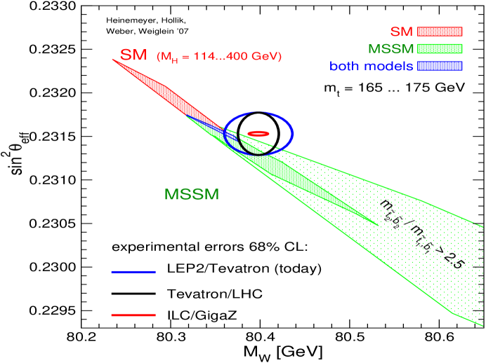
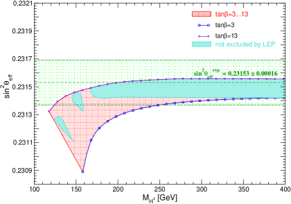
In Fig. 14 we compare the SM and the MSSM predictions for $\sin^{2}\theta_{\mathrm{eff}}$ as a function of $m_{t}$ as obtained from the scatter data. The predictions within the two models give rise to two bands in the $m_{t}$–$\sin^{2}\theta_{\mathrm{eff}}$ plane with only a relatively small overlap region (indicated by a dark-shaded (blue) area). The allowed parameter region in the SM (the medium-shaded (red) and dark-shaded (blue) bands) arises from varying the only free parameter of the model, the mass of the SM Higgs boson, from $M^{\textup{SM}}_{H}=114\,\,\mathrm{GeV}$, the LEP exclusion bound [104] (lower edge of the dark-shaded (blue) area), to $400\,\,\mathrm{GeV}$ (upper edge of the medium-shaded (red) area). The very light-shaded (green), the light shaded (green) and the dark-shaded (blue) areas indicate allowed regions for the unconstrained MSSM. In the very light-shaded region at least one of the ratios $m_{\tilde{t}_{2}}/m_{\tilde{t}_{1}}$ or $m_{\tilde{b}_{2}}/m_{\tilde{b}_{1}}$ exceeds 2.5, while the decoupling limit with SUSY masses of ${\cal O}(2\,\,\mathrm{TeV})$ yields the upper edge of the dark-shaded (blue) area. Thus, the overlap region between the predictions of the two models corresponds in the SM to the region where the Higgs boson is light, i.e., in the MSSM allowed region ($M_{h}\;\raisebox{-3.00003pt}{$\stackrel{{\scriptstyle\displaystyle<}}{{\sim}}$}\;130\,\,\mathrm{GeV}$ [43, 44]). In the MSSM it corresponds to the case where all superpartners are heavy, i.e., the decoupling region of the MSSM. The 68% C.L. experimental results for $m_{t}$ and $\sin^{2}\theta_{\mathrm{eff}}$ are indicated in the plot. As can be seen from Fig. 14, the current experimental 68% C.L. region for $m_{t}$ and $\sin^{2}\theta_{\mathrm{eff}}$ is in good agreement with both models and does not indicate a preference for one of the two models. The prospective accuracies for the Tevatron/LHC ($\delta\sin^{2}\theta_{\mathrm{eff}}^{\rm Tevatron/LHC}=0.00016$, $\delta m_{t}^{\rm Tevatron/LHC}=1\,\,\mathrm{GeV}$) and the ILC with GigaZ option ($\delta\sin^{2}\theta_{\mathrm{eff}}^{\rm ILC/GigaZ}=0.000013$, $\delta m_{t}^{\rm ILC/GigaZ}=0.1\,\,\mathrm{GeV}$) are also shown in the plot (using the current central values), indicating the strong potential for a significant improvement of the sensitivity of the electroweak precision tests [91].

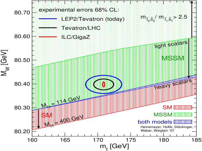
In Fig. 15 we compare the SM and the MSSM predictions for $M_{W}$ as a function of $m_{t}$ as obtained from the scatter data. The ranges of the varied parameters and the band structure of the SM and MSSM predictions are analogous to the ones in Fig. 14. The experimental value for $M_{W}$ includes the latest CDF measurement [106], resulting in the world average of $M_{W}=(80.398\pm 0.025)\,\,\mathrm{GeV}$ [106, 2]. The 68% C.L. region for $m_{t}$ and $M_{W}$ exhibits a preference for the MSSM over the SM. The prospective accuracies for the Tevatron/LHC ($\delta M_{W}^{\rm Tevatron/LHC}=15\,\,\mathrm{MeV}$) and the ILC with GigaZ option ($\delta M_{W}^{\rm ILC/GigaZ}=7\,\,\mathrm{MeV}$) are also shown in the plot (using the current central value).

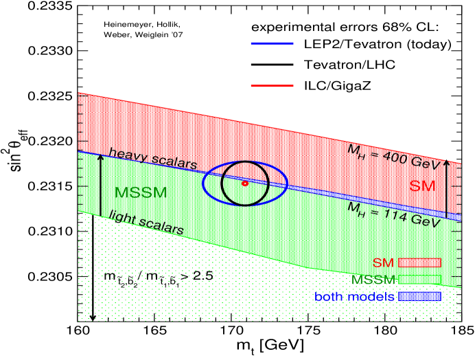
Finally in Fig. 16 we show the combination of $M_{W}$ and $\sin^{2}\theta_{\mathrm{eff}}$ with the top-quark mass varied in the range of $165\,\,\mathrm{GeV}$ to $175\,\,\mathrm{GeV}$. The ranges of the other varied parameters and the colour coding are the same as in Figs. 14, 15. The current 68% C.L. experimental results for $M_{W}$ and $\sin^{2}\theta_{\mathrm{eff}}$ are indicated in the plot. The region of the SM prediction inside todays 68% C.L. ellipse corresponds to relatively large $m_{t}$ values, outside the current experimental range of $m_{t}=(170.9\pm 1.8)\,\,\mathrm{GeV}$ [79]. Thus, the combination of $M_{W}$ and $\sin^{2}\theta_{\mathrm{eff}}$ exhibits a slight preference for the MSSM over the SM. Again also shown are the anticipated future improvements in the measurements of $M_{W}$ and $\sin^{2}\theta_{\mathrm{eff}}$.

6 Remaining higher-order uncertainties for $\sin^{2}\theta_{\mathrm{eff}}$

Following the discussion in Ref. [30] we now estimate the missing higher order uncertainties in the prediction of $\sin^{2}\theta_{\mathrm{eff}}$. As seen in Sect. 5, besides the $W$ boson mass, $\sin^{2}\theta_{\mathrm{eff}}$ is the observable with the most pronounced dependence on higher-order SUSY contributions. Thus, it is important to reduce its intrinsic theoretical uncertainty from unknown higher-order (SM and SUSY) correctins sufficiently below its experimental error and its parametric theoretical uncertainties (induced by the experimental errors of the input parameters). The remaining SM theory uncertainty was estimated to be [13, 16]

$$\delta\sin^{2}\theta_{\mathrm{eff}}^{\rm SM}=4.7\times 10^{-5}.$$ (84)

This corresponds to the theory uncertainty of our prediction for $\sin^{2}\theta_{\mathrm{eff}}$ in the decoupling limit of the MSSM, since we have incorporated all known SM higher order contributions into our result (see Sect. 4.3).

As detailed in Refs. [30, 28], additional theoretical uncertainties arise from higher-order corrections involving supersymmetric particles in the loops. Depending on the overall SUSY scale these uncertainties were estimated to be [28]

$$\delta\sin^{2}\theta_{\mathrm{eff}} = 4.7\times 10^{-5}\mbox{ for }M_{\tilde{f}}<500\,\,\mathrm{GeV},$$

$$\delta\sin^{2}\theta_{\mathrm{eff}} = 1.5\times 10^{-5}\mbox{ for }M_{\tilde{f}}=500\,\,\mathrm{GeV},$$ (85)

$$\delta\sin^{2}\theta_{\mathrm{eff}} = 1.3\times 10^{-5}\mbox{ for }M_{\tilde{f}}=1000\,\,\mathrm{GeV}.$$

Adding SM and SUSY uncertainties in quadrature one finds $\delta\sin^{2}\theta_{\mathrm{eff}}=(4.9\,-6.6)\times 10^{-5}$, depending on the SUSY mass scale [28].

Additional theory uncertainties arise for complex parameters, as we only include the full phase dependence at the one-loop level. However, MSSM two-loop terms which are only known for real MSSM parameters are incorporated into the full prediction for $\sin^{2}\theta_{\mathrm{eff}}$ via the interpolation relation eq. (60). Following the prescription in Ref. [30], where the corresponding error in the $M_{W}$ evaluation had been obtained, we estimate here the maximal error over the $\phi_{A_{t}}\in[0,\pi]$ interval to be

$$\delta\sin^{2}\theta_{\mathrm{eff}} = 2.6\times 10^{-5}\mbox{ for }M_{\tilde{f}}<500\,\,\mathrm{GeV},$$

$$\delta\sin^{2}\theta_{\mathrm{eff}} = 1.7\times 10^{-5}\mbox{ for }M_{\tilde{f}}=500\,\,\mathrm{GeV},$$ (86)

$$\delta\sin^{2}\theta_{\mathrm{eff}} = 0.6\times 10^{-5}\mbox{ for }M_{\tilde{f}}=1000\,\,\mathrm{GeV}.$$

Similar values are found in an independent approach: the approximation formula eq. (60) can be applied to the one-loop case, see Sect. 4.2.3. The difference between the approximation and the full phase dependence at one-loop order is scaled to the two-loop level by applying a conservative factor of 0.2 (obtained from the analyses of the SUSY contributions to the $\rho$ parameter [26, 28]). The result for the estimate of the uncertainty induced by the approximation formula for the phase dependence at the two-loop level is similar (slightly below) to the numbers in eq. (86).

The full theoretical uncertainty from unknown higher-order corrections in the MSSM with complex parameters can now be obtained by adding in quadrature the SM uncertainties from eq. (84), the theory uncertainties from eq. (85) and the additional SUSY uncertainties from eq. (86). This yields $\delta\sin^{2}\theta_{\mathrm{eff}}=(4.9-7.1)\times 10^{-5}$ depending on the SUSY mass scale.

The other source of theoretical uncertainties, besides the one from unknown higher-order corrections, is the parametric uncertainty induced by the experimental errors of the input parameters. The corresponding uncertainties for $\delta m_{t}=1.8\,\,\mathrm{GeV}$ and $\delta(\Delta\alpha_{\rm had}^{(5)})$ are given in eqs. (74) – (79). The uncertainty in $m_{t}$ will decrease during the next years as a consequence of a further improvement of the accuracies at the Tevatron and the LHC. Ultimately it will be reduced by more than an order of magnitude at the ILC [98, 99], see also the phenomenological analysis in Ref. [107]. For $\Delta\alpha_{\rm had}^{(5)}$ one can hope for an improvement down to $5\times 10^{-5}$ [100], reducing the parametric uncertainty to the $1.8\times 10^{-5}$ level (for a discussion of the parametric uncertainties induced by the other SM input parameters see, for example, Ref. [6]). In order to reduce the theoretical uncertainties from unknown higher-order corrections to the level of $1.8\times 10^{-5}$, further results on SM-type corrections beyond two-loop order and higher-order corrections involving supersymmetric particles will be necessary.

7 Conclusions

We have presented the currently most accurate evaluation of $Z$ pole observables in the MSSM. These comprise the effective weak mixing angle, $\sin^{2}\theta_{\mathrm{eff}}$, $Z$ decay widths to SM fermions, $\Gamma(Z\to f\bar{f})$, the invisible and total width, $\Gamma_{\rm inv}$ and $\Gamma_{Z}$, forward-backward and left-right asymmetries, $A_{\rm FB}$ and $A_{\rm LR}$, and the total hadronic cross section, $\sigma^{0}_{\rm had}$. The calculation includes the complete one-loop results, for the first time taking into account the full complex phase dependence. It furthermore includes all existing higher-order corrections available in the MSSM. We have also incorporated all available SM contributions that go beyond the existing MSSM corrections. These corrections can be numerically important since the evaluations of higher-order corrections in the SM are more advanced than in the MSSM. As a result, in the decoupling limit (i.e., if all SUSY mass parameters are large) our calculation reproduces the currently most up-to-date SM results for the $Z$ pole observables. Concerning the $Z$ boson decay widths we obtained for the first time a full one-loop result for $\Gamma(Z\to\tilde{\chi}^{0}_{1}\tilde{\chi}^{0}_{1})$ that contributes to the invisible width of the $Z$ boson if this decay is kinematically possible. A public computer code based on the results for electroweak precision observables (the $Z$ pole observables and the $W$ boson mass [30]) is in preparation [31].

We presented a detailed numerical analysis of the impact of the various MSSM sectors on the prediction of the EWPO. We find that the EWPO $M_{W}$, $\sin^{2}\theta_{\mathrm{eff}}$ and $\Gamma_{Z}$ are sensitive to variations of the $\tilde{t}/\tilde{b}$ sector parameters and to a lesser extent of the chargino/neutralino parameters. The impact on the other $Z$ pole observables was found to be much smaller and well within one experimental standard deviation. The evaluation of $M_{W}$ and $\sin^{2}\theta_{\mathrm{eff}}$ incorporating higher-order corrections to Higgs boson masses and couplings differs by about $1\,\sigma$ from the predictions where the tree-level approximation for the Higgs sector is used.

Particular emphasis in the analysis was put on the impact of the complex phases at the one-loop level. The largest phase dependence arises in general in the scalar top sector. Large effects are also possible in the scalar bottom sector if $\tan\beta$ is large. Shifts induced by a phase variation exceeding one experimental standard deviations can occur for $M_{W}$, $\sin^{2}\theta_{\mathrm{eff}}$ and $\Gamma_{Z}$, depending on the other MSSM parameters. It should be noted, however, that the dependence on the phases appearing in the $\tilde{t}/\tilde{b}$ sector at the one-loop level drop out of the explicit one-loop terms for the effective electroweak couplings $g^{f}_{\{V,A\},(1)}$ and thus only enter via their impact on the squark masses and mixing angles. Consequently, a measurement of the ${\cal CP}$-conserving EWPO alone cannot serve to reveal the presence of the complex phases. However, precise measurements of the EWPO in combination with other experimental information will be very valuable for constraining the SUSY parameters including the complex phases.

By comparing our MSSM result with the corresponding SM result we have illustrated the sensitivity of the EWPO to the virtual effects of SUSY particles. We pointed out that the anticipated experimental accuracy at future colliders, in particular at the ILC with GigaZ option, might resolve the virtual effects of SUSY particles, even in scenarios where the SUSY particles are so heavy that they escape direct detection at the LHC and the first phase of the ILC.

The EWPO have been analysed in the framework of several MSSM scenarios. As typical examples we investigated three SPS-like scenarios. Further studied scenarios were the “focus point” region, “split SUSY” and the CPX scenario. In the “focus point” and “split SUSY” scenarios, both containing heavy scalar fermions, only very small deviations from the corresponding SM result could be observed. Within the CPX scenario we found that the current experimental precision of the EWPO is not yet sufficient to probe the parameter space at low Higgs boson masses that could not be covered by the LEP Higgs searches.

Finally, we have analysed the theoretical uncertainty in the $\sin^{2}\theta_{\mathrm{eff}}$ prediction arising from the incomplete inclusion of complex phases beyond the one-loop level. Our estimate yields that this (additional) uncertainty can amount up to $2.6\times 10^{-5}$, depending on the SUSY parameters. The combination of this new uncertainty with the one estimated previously for the MSSM with real parameters yields an estimate of the intrinsic uncertainty of up to $7\times 10^{-5}$ for small SUSY masses.

The results derived for the purpose of this paper have already found application in various precision analysis projects [9, 10, 12], which are aimed at providing indirect constraints on the scale of supersymmetry based on current constraints from cosmology, $B$ physics, and electroweak precision data.

Acknowledgements

We thank G. Moortgat-Pick for interesting discussions concerning Sect. 5.5. We thank J. Erler and K. Mönig for discussions on the future experimental uncertainties of the $Z$ pole observables. We are further grateful to P. Bechtle for providing us with data to allow a detailed analysis of the CPX benchmark scenario. A.M.W. would like to thank the Instituto de Fisica de Cantabria (CSIC-UC), Santander for kind hospitality during part of this work. Work supported in part by the European Community’s Marie-Curie Research Training Network under contract MRTN-CT-2006-035505 ‘Tools and Precision Calculations for Physics Discoveries at Colliders’ (HEPTOOLS).

Appendix A Appendix

Here we show generic Feynman-diagrams contributing to the $Z$ pole observables in the MSSM.

A.1 One-loop vertex graphs for the process $Z\to f\bar{f}$

           

           

Figure 17: Generic vertex contributions to $Z\to f\bar{f}$.

A.2 SUSY QCD one-loop graphs for the process $Z\to q\bar{q}$

Figure 18: Generic SUSY QCD vertex contributions to $Z\to q\bar{q}$.

A.3 One-loop graphs for $Z\to\tilde{\chi}^{0}_{1}\tilde{\chi}^{0}_{1}$

           

           

Figure 19: Generic vertex contributions to $Z\to\tilde{\chi}^{0}_{1}\tilde{\chi}^{0}_{1}$.

A.4 SUSY two-loop graphs contributing to $\Delta\rho$

Figure 20: Sample diagrams for the SUSY ${\cal O}(\alpha\alpha_{s})$ contributions to $\Delta\rho$: $(g)$ squark loop with gluon exchange, $(\tilde{g})$ (s)quark loop with gluino exchange.

Figure 21: Sample diagrams for the three classes of MSSM ${\cal O}(\alpha_{t}^{2})$, ${\cal O}(\alpha_{b}^{2})$, ${\cal O}(\alpha_{t}\alpha_{b})$ contributions to $\Delta\rho$: $(q)$ quark loop with Higgs exchange, $(\tilde{q})$ squark loop with Higgs exchange, $(\tilde{H})$ quark/squark loop with Higgsino exchange. $\varphi$ denotes Higgs and Goldstone boson exchange.