KUNS-2105
Near Extremal Black Hole Entropy
as Entanglement Entropy via AdS2/CFT1
Tatsuo
Azeyanagi111e-mail:aze@gauge.scphys.kyoto-u.ac.jp,
Tatsuma Nishioka222e-mail:nishioka@gauge.scphys.kyoto-u.ac.jp and Tadashi
Takayanagi333e-mail:takayana@gauge.scphys.kyoto-u.ac.jp
Department of Physics, Kyoto University, Kyoto 606-8502, Japan
We point out that the entropy of (near) extremal black holes can be interpreted as the entanglement entropy of dual conformal quantum mechanics via AdSCFT1. As an explicit example, we study near extremal BTZ black holes and derive this claim from AdSCFT2. We also analytically compute the entanglement entropy in the two dimensional CFT of a free Dirac fermion compactified on a circle at finite temperature. From this result, we clarify the relation between the thermal entropy and entanglement entropy, which is essential for the entanglement interpretation of black hole entropy.
1 Introduction
The AdS/CFT [2] has been studied for almost ten years and many interesting aspects of quantum gravity have been revealed. Even though the examples of AdSCFTd with have been explored in detail, the lowest dimensional case has not been understood well even now. The AdS2 geometry appears as the near horizon limit of four or five dimensional extremal black holes (or black rings) [3, 4, 5]. Thus the microscopic explanation of Bekenstein-Hawking entropy of the extremal black holes [6, 7] is expected to be directly related to the AdSCFT1 correspondence [2, 8] (see [9] for a review).
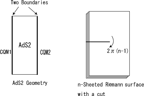
The pure AdS spacetime AdSd+1 with has no entropy as is also clear from its dual CFTd at vanishing temperature. To obtain non-zero entropy, we need to consider an AdS black hole as the dual geometry. On the other hand, we expect non-zero entropy even for the pure AdS2 since it is the near horizon limit of higher dimensional (near) extremal black holes. We also notice another special property of AdS2 that the AdSd+1 in the global coordinate has two (time-like) boundaries only when . The latter property has been a major problem when we would like to understand what the AdSCFT1 is because usually the CFT lives on the boundary of AdS space. So far this issue has been neglected and the AdS2 space is considered to be dual to a single CFT with a large degeneracy. Though it is also natural to assume that there are two CFTs, taking into account the presence of two boundaries on AdS2, there have been no arguments in this direction as far as the authors know.
In this paper, we would like to report a progress in this direction owing to the recently found method of holographically computing entanglement entropy [10, 11]. We point out that the above two exceptional properties of AdS2 are closely related with each other. We present an important evidence that there exist two systems of conformal quantum mechanics (CQM) on the boundaries of the AdS2 and that they are entangled with each other as is speculated from the non-vanishing correlation functions between them computed holographically. Indeed we will be able to show that the black hole entropy is exactly the same as the entanglement entropy of CQM if we assume the AdSCFT1 correspondence with this interpretation. This relation is true even if we take any higher derivative corrections into account. We can say that this progress is highly remarkable if we remember that the AdSCFT1 has been poorly understood and been still mysterious until now.
Even though our argument can be regarded as a generalization of the interpretation of AdS black holes in [12] via AdS/CFT, it is slightly different from it in the following point. For the (3D or higher dimensional) AdS black holes, its CFT dual is well established and it is possible to explicitly construct a dual entangled CFT state, from which we can compute its entanglement entropy directly as in [12]. On the other hand, in the AdS2 case, we can perform a computation of entanglement entropy in the dual CFT only by using the recent holographic method444This holographic method has also been applied to the analysis of the confining gauge theories [13, 14]. [10, 11] as the formulation of the dual CFT is not clear at present.
The relation between the black hole entropy and entanglement entropy has been discussed for a long time and historically this was the first motivation that makes us consider the entanglement entropy in quantum field theory [15]. Later, it turned out that quantum corrections to Bekenstein-Hawking formula can be explained as the entanglement entropy [16, 17]. In particular, when the entire gravity action is induced, the black hole entropy itself can be regarded as the entanglement entropy [17, 18]. In these arguments, the black hole entropy is related to the entanglement entropy in the quantum field theory in the same spacetime. The corresponding interpretation from the viewpoint of AdS/CFT has been given in [19, 20] (see also [21, 22, 23]). On the other hand, in our case, the black hole entropy is interpreted as the entanglement entropy in CFT (or CQM) which lives on the boundary of the spacetime .
Now, we usually identify the black hole entropy with the thermal entropy based on AdS/CFT. Thus in order to claim the equality between the black hole entropy and the entanglement entropy in general setups, we need to establish the relation between the thermal entropy and entanglement entropy. To see that it indeed agrees with what we expect from the holographic viewpoint, we compute the entanglement entropy of a 2D free Dirac fermion at finite temperature with the spatial direction compactified as an explicit example. We finally obtain an analytical expression and are able to check this relation. This is the first analytic result on entanglement entropy with both the finite temperature and finite size effect taken into account555Since this result may also be interesting for those who are interested in other subjects, we arranged such that the section 5 is readable for anyone who is familiar with 2D CFT.. Also remarkably, in our setup the entanglement entropy depends on the detail of the 2D CFT, while the entanglement entropy at zero temperature or in the infinite system only depends on the central charge of CFT [24, 25].
This paper is organized as follows: In section 2 we explain the holographic computation of entanglement entropy via the AdS/CFT duality. We also presents a new evidence of this relation in the BTZ black holes. In section 3, we give a general argument to show the equivalence between the black hole entropy and the entanglement entropy via AdSCFT1. In section 4, we investigate near extremal BTZ black holes in order to derive our claim from AdSCFT2. In section 5, we analytically compute the entanglement entropy of a 2D free Dirac fermion at finite temperature with the spacial direction compactified. In section 6, we draw a conclusion and discuss future problems.
2 Holographic Entanglement Entropy and BTZ Black Holes
The main purpose of this paper is to understand the AdS2/CFT1 better by uncovering the relation between the black hole entropy and the entanglement entropy in CFT1. However, it is quite useful to learn a general holographic prescription of computing entanglement entropy from the AdS/CFT correspondence. This is because the dual CFT in AdS2/CFT1 is not understood well and we need to employ a holographic computation of the entanglement entropy666Again please distinguish this entanglement entropy in CFT1 from the entanglement entropy in AdS2. for CFT1. We will apply this general method to the AdS2/CFT1 setup in the next section. Also in a particular case of AdS2 background in string theory can be embedded into a rotating BTZ black hole, which is asymptotically AdS3 as we will see.
Motivated by this, we will explain the general holographic computation of the entanglement entropy [10] in this section. Especially we study the example of BTZ black holes and its CFT2 dual based on the AdS3/CFT2 and present a new result. This gives a further evidence that the general prescription in [10] correctly reproduces the black hole entropy as the entanglement entropy. Also the entropy of BTZ black hole is closely related to the entropy of extremal black holes which is the main topic of this paper as we will see later.
2.1 Holographic Entanglement Entropy
Consider a CFT and divide the space manifold of the CFT into two parts and . This factorizes the total Hilbert space into a direct product of two Hilbert spaces . The entanglement entropy is defined by the von-Neumann entropy for the reduced density matrix . The reduced density matrix is defined by tracing out the density matrix over i.e. . We have an infinitely many such quantities for various choices of .
Now we would like to compute the entanglement entropy from the AdS/CFT correspondence. We assume a setup where a AdSd+2 space with the Newton constant is dual to a CFTd+1. The CFT lives on the boundary of AdS. Then the general holographic prescription in [10] computes the entanglement entropy as the area of the minimal surface at a constant time
| (2.1) |
where is the (unique) minimal surface in AdSd+2 whose boundary coincides with the boundary of the region A. A simple proof of this claim has been given in [26]. Notice that this formula assumes the supergravity approximation of the full string theory.
2.2 Application to BTZ Black holes
As a particular example, which is also relevant to the discussions in the next section, let us consider the BTZ black holes [27], whose metric is given as follows
| (2.2) |
The boundary of BTZ black hole at a fixed time is a circle because has the periodicity . The entanglement entropy is defined by dividing this circle into two parts and . We specify the size of by the angle , while the size of becomes .
If we apply the holographic formula (2.1) to BTZ black holes, is equal to the geodesic length between the two endpoints of inside the bulk space. This holographic computation leads to the following prediction [10]
| (2.3) |
where is the central charge of the dual CFT2 and is the inverse temperature of the black hole. This agrees with the result in [25], which computes the entanglement entropy in any 2D finite temperature CFT when the size is small. However, when is large, the formula (2.3) is no longer correct as will be clear from the holographic consideration discussed just below.
At high temperature, the geodesic winds around the black hole horizon as becomes large (Figure 1(a)). When the region covers most of the boundary ( with ), the disconnected surface (Figure 1(c)) gives smaller area than777Remember that when the temperature is non-vanishing but is not high enough, the AdS/CFT claims that the dual gravity description is given by the path-integral over infinitely many geometries as in [28, 29]. Thus our results such as (5.17) and (5.24), which are correct for any values of , should include such a sum over geometries. the connected surface (Figure 1(b)). Thus the disconnected surface consists of the total black hole horizon and the geodesic extending to the boundary. Taking the limit, this leads to
| (2.4) |
where is the black hole entropy. This relation (2.4) offers an important way to extract the black hole entropy from the entanglement entropy of CFT2.
Therefore it is very important to confirm (2.4) from the CFT side without assuming AdS/CFT. Indeed in section 5.3 we will show this is indeed true for a particular CFT. There, we consider the example888In this subsection, we have proceeded by pretending that the free Dirac fermion system has its AdS dual. We believe this assumption is not crucial because the property (5.19) should be true for any 2D CFT. It is well-known that the IIB string on AdS ( or ) is dual to the 2D SCFT defined by the symmetric orbifolds . Thus it will be an interesting future problem to extend our calculations of entanglement entropy to the ones in symmetric orbifolds and see that the result can explicitly be interpreted as the sum over geometries. of free fermion CFT since it turns out to be possible to compute the entanglement entropy analytically and show this relation as in (5.22).
In this way we have been able to understand well the BTZ black hole entropy from the viewpoint of entanglement entropy. This gives a further evidence of AdS3/CFT2. In the next sections, we would like to proceed to another important class of black holes i.e. the ones whose near horizon geometry includes the AdS2.

|

|

|
3 Black Hole Entropy as Entanglement Entropy and AdS2/CFT1
3.1 AdS2 from the Near Horizon Limit of Extremal Black Hole
The metric of a 4D charged black hole looks like
| (3.1) |
where we assumed . The Bekenstein-Hawking entropy is given by
| (3.2) |
The extremal black hole corresponds to the special choice of the parameter . In this case, if we define , the near horizon metric becomes
| (3.3) |
i.e. AdS2 in the Poincare coordinate times .
More generally, it is possible to obtain AdS when the black hole is near extremal [30]. In this case, the dual ground state in AdS2 is heated up into a thermal state so that its temperature is proportional to . As we will see in the last part of the next section, the extremal black hole behaves differently from the near extremal one especially in the global structure of the spacetime. Below we mostly consider the extremal limit of the near extremal black hole instead of the extremal one itself.
As is well known, the AdS2 in the global coordinate
| (3.4) |
has a significant difference from the higher dimensional AdS spaces in that it has two time-like boundaries at . Thus it is natural to expect that the theory is dual to two copies of conformal quantum mechanics CQM and CQM living on the two boundaries via AdS2/CFT1. In the next section, by considering 5D (near) extremal black holes, we will give an explicit example of AdS2/CFT1 duality, which supports this interpretation.
In the case of 4D extremal black holes, the systematic construction of dual CQM has not been established. There are some specific examples whose dual quantum mechanics is understood [31, 32, 33]. Instead of the detailed review of each examples, we would like to briefly give a sketchy explanation since the detail is not necessary for our purpose. Consider the setup of type IIA string compactified on a Calabi-Yau 3-fold with D-branes and D-branes. We specify the number of D-branes and D-branes wrapped on the 4-cycle by and . This configuration leads to a macroscopic BPS black hole with the entropy in a large charge limit, where in terms of the intersection number [34]. In the near horizon limit, the geometry AdS is realized. In this setup, the dual quantum mechanics is described by a supersymmetric sigma model whose target space is the symmetric product of a certain manifold [31]. This manifold represents the effective geometry of D4-brane world-volume probed by a D-brane. The number of ground states of this model is equal to the number of cohomology of the symmetric product . We can apply the orbifold formula as usual to count [35, 6]. This turns out to be equivalent to the counting of left-moving states of a two dimensional CFT at level with the central charge [31, 34]. This reproduces . In this setup, we can regard the pair CQM1 and CQM2 as the two copies of the symmetric product quantum mechanics.
3.2 Holographic Computation of Entanglement Entropy
Since there are two CQMs, it is natural to ask if there are any correlations between them. We can compute from the standard bulk-boundary relation [36] the two point function between in CFT1 and in CFT2 as follows (we assume the global AdS2 (3.4))
| (3.5) | |||
| (3.6) |
where is the conformal dimension of the operator .
At first, one may think they are decoupled because the CQM1 and CQM2 are disconnected. However, as the non-vanishing two point functions show, AdS/CFT predicts they are actually correlated. A similar puzzle has been raised in [37] in the context of AdS wormhole. Indeed the following discussion is closely related to the holographic computation of entanglement entropy in AdS wormholes [11].
In this paper we would like to claim that CQM1 and CQM2 are actually quantum mechanically entangled with each other and that this is the reason why we get the non-vanishing correlators. To show that the two CFTs are entangled, we need to compute the entanglement entropy and to check that it is non-zero. Below we would like to calculate the entanglement entropy holographically.
The holographic formula (2.1) is expected to be true in general AdS space. If we apply it to our AdS2 setup (i.e. d=0 in (2.1)), we naturally find
| (3.7) |
This is because the minimal surface now becomes a point. Below we will give a clearer derivation of (3.7) based on the AdS/CFT.
The Hilbert spaces of CQM and CQM are denoted by and . The total Hilbert space looks like . We define the reduced density matrix from the total density matrix
| (3.8) |
by tracing over the Hilbert space . This is the density matrix for an observer who is blind to CQM. It is natural to assume that is the one for a pure state.
The entanglement entropy for CQM, when we assume that the opposite part CQM is invisible for the observer in CQM, is defined by
| (3.9) |
We can obtain this by first computing Tr, taking the derivative w.r.t. and finally setting . In the path integral formalism of the quantum mechanics, and Tr are computed as in Figure 2 (we perform the path-integral along the thick lines. and are the boundary conditions.).
By using the bulk-boundary relation of AdS/CFT [36], we can compute the entanglement entropy holographically as in the right of the Figure 3. The dual geometry is the -sheeted Riemann surface [10]. Though our derivation below is along the line with the argument in [26] for which proves the claim in [10] via the bulk to boundary relation [36], our example is more non-trivial as it includes two boundaries. Also it is closely related999Notice that in these arguments the authors consider the entanglement entropy for the total spacetime of non-extremal black holes, while in our argument we consider the entanglement entropy for the boundary of the extremal black hole geometry. to the conical defect argument of black hole entropy (see e.g. [18, 38]).
Here we are considering an Euclidean metric. The cut should end on a certain point in the bulk because there should not be any cut on the opposite boundary, which is first traced out. Notice that the presence of two boundaries in AdS2 plays a crucial role in this holographic computation. We would get the vanishing entropy if we were to start with the spacetime which has a single boundary such as the Poincare metric of AdS2.
Now we remember the Einstein-Hilbert action in the Euclidean space
| (3.10) |
The cosmological constant is not important since it is extensive and it will vanish in the end of the entropy computation. In the -sheeted geometry we find in the Euclidean formalism because the curvature behaves like a delta function (see e.g.[26, 38]). The entanglement entropy is obtained as follows
| (3.11) |
where is the value of Einstein-Hilbert action of a single-sheet in the absence of the cut (or negative deficit angle).

Finally, it is trivial to see that
| (3.12) |
because . This means that the entanglement between CQM and CQM is precisely the source of the 4D (near) extremal black hole entropy. The same argument can be applied to any dimensional black holes or black rings whose horizons are of the form AdS, where is a compact manifold such as .
Recently, it has been shown that extremal (rotating) black holes always have the symmetry in the near horizon limit [3, 4, 5]. For example, the near horizon geometry of a four dimensional extremal Kerr black hole is given by a warped product of AdS2 and a two dimensional manifold [39]. Our argument in this subsection can be applied to such a warped AdS2 case.
3.3 Higher Derivative Corrections
Moreover, we can take curvature corrections into account. We assume that the near horizon geometry is of the form AdS. Even though we start with the Lagrangian that includes the curvature tensor and their covariant derivatives, we can neglect the covariant derivative of curvature tensors because the near horizon geometry has the constant curvature. In this case, the black hole entropy with the curvature corrections is given by the Wald’s formula [40, 41]
| (3.13) |
where by using the Killing vector of the Killing horizon and its normal , normalized such that ; represents the horizon and is the metric on it.
For example, in the ordinary Einstein-Hilbert action , we reproduce the standard result
| (3.14) |
where is the horizon area.
Now we would like to compare the Wald entropy with the entanglement entropy computed holographically via AdS2/CFT1. We consider the -sheeted AdS2 (times the same ), where the Riemann tensor behaves as follows [38]
| (3.15) |
Here is the delta function localized at the (codimension two) horizon; represents the constant curvature contribution from the cosmological constant. run the coordinate in the AdS2. Notice also that if we employ the relation , we obtain
| (3.16) |
Now we consider the perturbative expansions of the Lagrangian with respect to the (delta functional) deviation of from . Then the quadratic and higher order terms do not contribute since for . Therefore, we can find
| (3.17) | |||||
Thus this agrees with the Wald’s formula
| (3.18) |
3.4 Towards Holography in Flat Spacetime
For general non-extremal black holes,
| (3.19) |
we obtain a Rindler space in the near horizon limit . The global extension of the Rindler space is clearly the two dimensional Minkowski spacetime . Thus we cannot relate it to the AdS/CFT correspondence.
If we associate two quantum mechanical systems, however, to two time-like curves situated at the left and right side of , then we can obtain the same equality as (3.12). This suggests that the flat Minkowski spacetime may admit its holographic description. It also has a natural higher dimensional extension by expressing the metric as , where is the metric of the dimensional de-Sitter space.
4 The AdSCFT1 Duality from 5D Near Extremal Black Holes
In the previous section we have argued that the black hole entropy of (near) extremal black hole whose near horizon geometry includes a AdS2 factor, is equal to the entanglement entropy of two dual CQMs, including quantum corrections. We confirmed this claim by assuming the AdSCFT1. To obtain a complete proof, we need to explicitly present a general construction of the entangled pair of CQMs. In the 4D black hole cases, this is not straightforward because the CQM dual to AdS2 has not been well understood at present.
Instead, in this section we would like to examine a concrete example of AdSCFT1 which is obtained from the near extremal limit of non-rotating 5D black holes. Equally we can regard this as a dimensional reduction of AdSCFT2 as first pointed out in [8] since the near horizon geometry of 5D near extremal black holes is a rotating BTZ black hole [27, 42] (see also [28]).
4.1 Near Extremal BTZ Black Hole from 5D Black Holes
Consider a 5D black hole which is obtained from the type IIB background with D1-branes and D5-branes wrapped on with Kaluza-Klein momentum in the direction. In the near horizon limit, the metric becomes [7]
| (4.1) |
Via a coordinate transformation we can show that this geometry is equivalent to [28]
| (4.2) |
The metric of the rotating BTZ black hole metric [27, 42] is given by (2.2). The explicit coordinate transformation is given by
| (4.3) |
and the new parameters are defined as . We can take if we choose , where is the radius of .
This BTZ geometry (2.2) can also be obtained from a Lorentzian orbifold of the pure AdS3 space
| (4.4) |
They are related by the coordinate transformation
| (4.5) |
The periodicity of (i.e. ) leads to the identification
| (4.6) |
where and represent the left and right-moving temperature of the dual 2D CFT. The central charge of dual CFT is given by and its density matrix looks like
| (4.7) |
using the left and right-moving energy and .
In the extremal case , we need another coordinate transformation defined by
| (4.8) |
The periodicity of is equivalent to
| (4.9) |
The thermal entropy of the dual CFT is given by the standard formula and this agrees with the black hole entropy , using the thermodynamical relation .
4.2 From Near Extremal BTZ to AdS2
The near extremal 5D black hole is related to the near extremal BTZ black hole . In the dual CFT, the left moving sector is far more excited compared with the right-moving sector since .
By considering the limit of the BTZ metric (2.2), we define and assume . In the end we find the simplified metric
| (4.10) |
The 2D part of (4.10) is equivalent to the ’AdS2 black hole’ defined in [30]
| (4.11) |
where
| (4.12) |
We can show that this space is equivalent to the pure AdS2 via a coordinate transformation [30]. Though the temperature dependence disappears by this transformation, it reflects the choice of different thermal vacua [30]. Thus the 3D background (4.10) is equivalent to AdS.
In order to have a sensible interpretation in terms of AdS2/CFT1, the geometry should include the boundary region of the AdS2 dual to the UV limit of CFT1. This is given by the region . On the other hand, the approximation to get (4.10) assumes the condition . Thus we have to require
| (4.13) |
This means that we cannot neglect the excitation in the direction of the spacetime AdS. However, still we can perform the Kaluza-Klein reduction and regard the theory as the one on AdS2 with infinitely many Kaluza-Klein modes.
The generators101010Notice that we distinguish from the standard basis dual to the Virasoro generators of 2D CFT. In our case, the unbroken generators of and are linear combinations of the standard Virasoro generators. and of the isometry of the AdS3 in the Poincare coordinate (4.4) are given by
| (4.14) |
and their anti-holomorphic counterparts obtained by exchanging with . For states dual to generic BTZ black holes, the two symmetries are both broken. However, if we take the limit (i.e. (4.13)) of the extremal BTZ , we can keep (i.e. and ) unbroken as is clear from the orbifold action (4.9) on the expressions (4.14). The generator is the translation in the direction and the right-moving symmetry turns out to be essentially the same as the isometry of the AdS2 [8].
This analysis of the conformal symmetry reveals that the excitation in the direction is related to the left-moving sector. Thus we can regard this AdSCFT2 as a variant of AdSCFT1 by treating the left-moving sector as an internal degree of freedom. Notice that excitations in the left-moving sector do not shift the value of the Hamiltonian for CFT1 (i.e. ). Thus the conformal quantum mechanics dual to AdS2 is essentially described by the right-moving part of CFT2.
This suggests a DLCQ interpretation of the dual CFT. In order to properly normalize the metric (4.10) in the limit (4.13), we are lead to define
| (4.15) |
Thus in this picture we can equivalently regard that the CFT2 is almost light-like compactified and . In this description, it is easy to confirm the unbroken symmetry because is scaled as and gets insensitive under the orbifold action. Also this rescaling shifts the energy scale we are looking at as . This agrees with the near extremal limit that we have been assuming so far. Notice also that in this limit the time evolution is equivalent to the one of the light-cone time and therefore the right-moving energy is treated as the Hamiltonian.
4.3 Two Point Functions
In order to have a better understanding of the AdSCFT1 interpretation of the near extremal BTZ black hole, we would like to turn to the two point function computed holographically following the bulk to boundary relation [36].
The Feynman Green function of a scalar field in global AdS3 is given in [43] and also that in BTZ can be constructed by the orbifold method. AdS3 is defined as the three dimensional hyperboloid embedded in and its metric takes a form . In the global AdS3, the Green function takes fairly simple form like
| (4.16) |
where
| (4.17) |
If we define the coordinate
| (4.18) |
we obtain the Poincare coordinate (4.4). The parameter in the above coordinate becomes
| (4.19) |
and by substituting this to (4.16), we obtain the Green function in the Poincare coordinate.
Considering the images which come as a result of the orbifolding procedure, the Green function in the rotating BTZ becomes
| (4.20) | |||||
| (4.21) | |||||
where
| (4.22) |
Now we would like to reduce the previous bulk-bulk Green functions to the AdS2 ones. Notice that the geodesic length can always be taken to be very large since we can consider two points near the boundary of AdS2 owing to (4.13). Thus the Green function looks like
| (4.23) |
Consider again the near extremal BTZ and take the limit . Then we obtain
| (4.24) | |||||
In this case the holographic two point function in the AdS2 limit looks like (below we omit numerical constants)
| (4.25) |
This takes the same expression as the one of holographic two point function of CFT2 [45, 46]. In the DLCQ coordinate, this is rewritten as follows
| (4.26) |
In the DLCQ coordinate, we treat as the basic coordinates and thus in the scaling (4.13) we can set in the above summation. Then the left and right-moving sector are decoupled as expected. Notice that the coordinate in the direction is .
To interpret the near horizon limit of near extremal BTZ (i.e. AdS) from the viewpoint of the AdSCFT1, we need to regard the left-moving sector dual to the part as an internal degree of freedom as we have explained before. This allows us to treat as a label of internal quantum number. Thus we can extract the two point function of CFT1 from (4.26) as follows
| (4.27) |
Here we have employed the relation , which is obtained from the infinite boost (4.15). This behavior agrees with the result for the thermal state in AdS2 [30]. Especially, in the extremal limit we find
| (4.28) |
as expected. In this way we have confirmed that we can regard the AdSCFT2 correspondence for the near extremal BTZ black hole equally as the AdSCFT1 with infinitely many internal degrees of freedom.
4.4 Quantum Entanglement and Black Hole Entropy
As we have explained, the AdSCFT2 correspondence for the near extremal black holes can also be regarded as a AdSCFT1 by taking the near horizon limit of the near extremal BTZ black hole. Essentially, the CFT1 i.e. the conformal quantum mechanics is described by the right-moving sector of the original CFT2 by treating the left-moving one as an internal degree of freedom tensored with the right-moving sector. When we consider the excitation in the AdS2 spacetime with the sector untouched, the left-moving sector will always stay at , where is the quantized momentum in the original 5D black hole description.
Usually, the CFT dual of the rotating BTZ black hole is interpreted as a thermal state. Equally we can interpret this as an entangled state in two copies of the same CFT [12]
| (4.29) |
where is the partition function of the 2D CFT. In the gravity side, they are geometrically understood as the CFTs living on the two disconnected boundaries of the BTZ spacetime.
To describe near extremal BTZ black holes, we keep finite and very large. In the near horizon limit , two boundaries of BTZ descend to the direct product of the two boundaries of AdS2 times the circle . We denote the states with by . The number of such states is very large . Then the quantum state looks like
| (4.30) |
where is the energy of the CQM.
Consider the zero temperature limit . Then the right-moving sector has a single ground state . The reduced density matrix of CQM1 , which is obtained by tracing over CQM2, now becomes
| (4.31) |
where . This leads to the following entanglement entropy
| (4.32) |
This clearly agrees with the familiar microscopic counting of BPS states and thus is equal to the black hole entropy [7]. We can also confirm that it agrees with the entanglement entropy calculated holographically for the near horizon geometry AdS of 5D (near) extremal black holes. In this way, we have shown that the AdSCFT1 description correctly reproduces the black hole entropy of (near) extremal 5D black holes.
We would like to stress that the density matrix (4.31) shows that the two quantum mechanics are maximally entangled. In general it is possible to find a quantum state with a smaller value of entanglement entropy even if the number of degeneracy is . However, the entropy of extremal black holes known so far has always been explained by assuming maximally entangled states.
4.5 Subtlety of the Extremal Limit
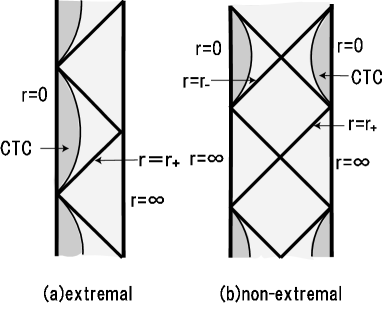
In this section we have mostly treated the extremal BTZ black holes as a limit of non-extremal ones, instead of starting with the extremal ones themselves. This is because the extremal limit looks sometimes subtle. This subtlety of defining extremal black hole entropy has been noticed for a long time [44].
First of all, this subtlety is noticed from the different forms of Penrose diagrams (Figure 4) [42]. In both extremal and non-extremal case, there are two boundaries in the Penrose diagram. Thus one may think that they should be interpreted as the two entangled CFTs. However, in the extremal case one of the two boundaries always includes the closed time like curve (Figure 4(a)), while in the non-extremal case not (Figure 4(b)). As far as we consider the non-extremal case, we can find the same boundary structure in the opposite boundary (as in Figure 4(b)) and thus we can apply the interpretation111111It is often claimed that we cannot extend the rotating black hole spacetime beyond the inner horizon [12, 47, 48]. Our derivation of black hole entropy from the holographic entanglement entropy done in section 2 is still fine even if we take this restriction into account. of two entangled CFTs [12, 45, 46, 47, 48, 49].
In the extremal case, we find only one boundary which has the sensible property with the CFT dual. Therefore one may worry that the entangled interpretation is confusing in the strictly extremal case. On the other hand, most of physical quantities of extremal black holes such as two-point functions are obtained smoothly by taking the extremal limit of those of the non-extremal ones. Therefore, if we apply the previous analysis in the non-extremal case to the extremal case, we will get the same conclusion; the CFT dual to the extremal case is described by the entangled states. Refer also to the argument in [49] for an interesting candidate of a geometrical interpretation of these entangled pairs via AdSCFT2.
Even though we cannot completely resolve the mentioned conflict with the global geometry, the holographic consideration leading to (4.31) via AdSCFT2, tells us that the entangled interpretation is still correct even for strictly extremal black holes. Also notice that in the near horizon limit , we do not have to worry about this problem. This is because the near horizon geometry of the extremal case has no closed time-like curve and two regular boundary CFTs are recovered in this limit. It will be an interesting future problem to explore this point.
5 Finite Size Corrections of Entanglement Entropy at Finite Temperature
In this section we compute the entanglement entropy of a 2D free Dirac fermion at finite temperature when the spatial direction is compactified (to unit radius). This is the first analytical result of the entanglement entropy for a finite size 2D CFT at finite temperature. In the case of either infinite size or zero temperature, the expression of entanglement entropy becomes very simple and takes the form of the central charge times a universal function as found in [24, 25]. However, in our case, the entanglement entropy depends more sensitively on the theory we consider.
In section 2, we have seen that the relation (2.4) is very important for the understanding of BTZ black hole entropy in AdS3/CFT2. This important relation between thermal entropy and entanglement entropy can only be explicitly shown in a finite size system. Indeed the behavior of the entanglement entropy agrees with what we expect from the geometric picture obtained from the AdS/CFT explained in section 2. This supports our claim that the black hole entropy is interpreted as the entanglement entropy in the dual CFT.
5.1 Two Point Function of a Compactified Boson
To make calculations simple, we consider the entanglement entropy of a free Dirac fermion . This fermion is bosonized into a scalar field with the unit radius as . We assume the Euclidean 2D theory on a torus defined by and since we are interested in a finite temperature theory with a finite size. In particular, when the period is pure imaginary , the theory is at the temperature and its spacial size is .
The primary operator denotes the one with the momentum and the winding such that the chiral dimension becomes and .
In particular, we are interested in a Dirac fermion, which is equivalent to the real boson at the radius . For example, the one-loop partition function is transformed as follows
| (5.2) | |||||
In this way the free boson partition function is decomposed into the four sectors , , and , each corresponds to of the theta function as usual.
5.2 Calculating Entanglement Entropy
In general, to compute the entanglement entropy, we first divide the total system into two subsystems and . In our setup, we define (or ) to be an interval with length (or ) at a specific time. Next, we compute Tr, where is the reduced density matrix obtained by taking a trace of the density matrix over the subsystem i.e. . This is usually possible by assuming is an positive integer. Then we analytically continue with respect to . Finally we take the derivative of and obtain the entanglement entropy of the subsystem
| (5.3) |
We can calculate Tr by employing the following formula which relates it to a product of two point functions of twisted operators [51, 10]
| (5.4) |
with the understanding of .
We identify the twist operator with the operator which has the fractional winding number so that the fermion picks up the phase if it goes around the two end points and . By setting , we find the extra phase becomes
| (5.5) |
Thus the two point function (5.1) in the sector of the fermion becomes
| (5.6) |
where . Below we assume that is pure imaginary except in section 4.7.
Now the entanglement entropy can be found by applying (5.3) and (5.4) to (5.6). To make the presentation simpler, we divide the entropy into two parts
| (5.7) |
where is the one from the first factor in the right-hand side of (5.6), while is from the second factor.
It is easy to calculate since the expression depends on only via the conformal dimension (in our model the central charge is given by ). We obtain
| (5.8) |
The exact expression suitable for the low temperature expansion is given by
| (5.9) |
where . The expression of high temperature expansion is obtained from the modular transformation as follows
| (5.10) |
where . Notice that this contribution satisfies
| (5.11) |
Secondly, is given by
| (5.12) |
In order to perform an analytical continuation with respect to we need to complete the summation of . This can be done by expanding the logarithm in (5.12) explicitly by employing the standard formula as we will see in the next subsection.
5.3 High Temperature Expansion
We first restrict to the special case , i.e. the NS sector for simplicity. We will come back to other spin structures in section 5.7.
Let us evaluate in the high temperature expansion. In order to get the high temperature expansion, we need to perform the modular transformation
| (5.13) |
Then we obtain
| (5.14) |
where the part is found to be
| (5.15) | |||||
In this calculation we have employed the following formula
| (5.16) |
In summary, the total expression of in the high temperature expansion becomes
| (5.17) | |||||
In this final expression, we make the dependence on the UV cut off explicit. We plotted the function (5.17) in Figure 5 by setting and .
The first factor reproduces the known result in the infinite size limit [25]. This part is successfully reproduced from the holographic dual computation in a BTZ black hole via AdS/CFT in [10].

By taking the limit , we find
| (5.18) |
Thus we can extract the finite part
| (5.19) |
Clearly, the leading term represents the thermal entropy in the high temperature limit .
On the other hand, the full expression of thermal entropy is given by
| (5.20) | |||||
where the partition function is defined by
| (5.21) |
Remarkably, we can show that the total expression of (5.19) indeed agrees121212 This proof is elementary. with the thermal entropy for arbitrary
| (5.22) |
This relation is very clear in the holographic picture based on AdS/CFT as will be explained in section 2.2.
5.4 Low Temperature Expansion
On the other hand, it is possible to perform the low temperature expansion with the modular transformation undone. In the end, we obtain similarly to (5.15)
| (5.23) | |||||
In summary, the total expression of entanglement entropy in the low temperature expansion becomes
| (5.24) | |||||
At zero temperature, the formula (5.24) is simply reduced to
| (5.25) |
and this reproduces131313Remember that we assume the space coordinate is compactified on a circle whose length is . the known result [25]. This part is successfully reproduced from the holographic dual computation via AdS/CFT in [10].
Still one may worry if there are many poles which come from the final term in (5.24). However, this turns out to be an artifact of the order of the summation as we will see in the next subsection. Indeed, the high and low temperature expansion will be proved to be equivalent as they should be. The high temperature expression is suitable for numerical computations.
5.5 Comparison of High and Low Temperature Expansion
Originally, the low and high temperature expressions of entanglement entropy come from the same two point function (via the modular transformation) and thus they are at least formally equivalent. However, as we have mentioned, they do not appear to be so at first sight.
In spite of this, we can show that when they are expanded with respect to the powers of like
| (5.26) |
each coefficient agrees with each other i.e. . Thus the point is the order of summations.
Let us present the proof of the equivalence. By applying the series expansions ( are Bernoulli numbers)
| (5.27) |
to (5.24) and (5.17), the equalities are rewritten as follows
| (5.28) |
These are equivalent to the relations
| (5.29) |
where we defined
| (5.30) |
They can be proven by considering the integral representation
| (5.31) |
where represents the path (Figure 6). It is easy to show (5.30) by summing over the residues of poles .
By deforming into which surrounds the poles on the imaginary axis , we can indeed prove (5.29) directly (only when we need to take into account the pole at ).
In this way we have found that the low and high temperature expansion are equivalent. For the actual computation the high temperature expansion is more useful.

|

|
5.6 Generalization
Here we would like to generalize the above result to the case in which the interval extends not only in the spacial direction but also in the temporal direction by setting , where is the Euclidean time. We also treat as a general complex number so that it includes the rotating black holes after the Lorentzian continuation. Remarkably, the entanglement entropy becomes the sum of the holomorphic contribution and the anti-holomorphic one as the thermal entropy does.
Generalization is straightforward since we have only to replace and in the previous results. The two point function of twist operators becomes
| (5.32) |
In the following calculation, we restrict to as above.
We firstly evaluate in the high temperature expansion. is
| (5.33) | |||||
where represents
| (5.34) |
with and is complex conjugate of the first term which comes from the anti-holomorphic part. is calculated as
| (5.35) |
As a result we have
| (5.36) | |||||
where we made the cut off explicit.
The expression of in the low temperature expansion is also given as
| (5.37) | |||||
where . Here the first term and the second one are contributions from the holomorphic part of and respectively.
5.7 Other Spin Structures
It is also useful to find the entanglement entropy for other spin structures of the Dirac fermions. First consider the case of i.e. the finite temperature theory with the periodic boundary condition (R sector). To calculate the entanglement entropy in the high temperature expansion, we again apply the modular transformation and obtain (the other parts are the same as case)
| (5.38) |
In this case, the thermal entropy defined by (5.20) becomes
| (5.39) |
and we can check agrees with this.
It is also possible to compute the entanglement entropy in the case. This corresponds to the index calculation in the NS sector Tr and is not related any realistic thermal distribution. In this case, similarly we obtain
| (5.40) |
In limit, (5.15) and (5.40) vanish respectively. This implies the boundary condition in the thermal direction can be neglected in this limit as expected. The thermal entropy is
| (5.41) |
and we can check that agrees with this.
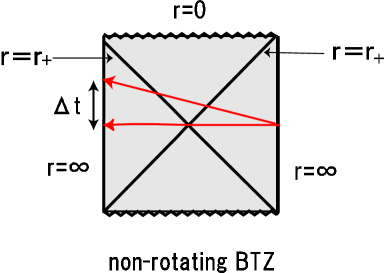
5.8 Temporal Entanglement Entropy: Beyond the Horizon
For simplicity, here, we take which corresponds to the case of non-rotating black hole. It is worth while to take some notice the case in which in the above generalization. The imaginary shift of the Lorentzian time takes us from a boundary to the other boundary [45, 46] (see Figure 7).
When is sufficiently small, using the high temperature expansion, we find
| (5.42) |
This entanglement entropy can be calculated also from the bulk geodesic point of view since it is related to the bulk geodesic distance between the points in which the twist operators are inserted [10] as in (2.1). The bulk geometry is the non-rotating BTZ black hole and the Penrose diagram is in Figure 7. The metric follows from (2.2) by taking and . The geodesic which corresponds to the above calculation can be seen in the Figure 7. Here we set at the initial point. The geodesic distance can be exactly found [46]
| (5.43) |
Since the central charge is given by [52], we can precisely show the equality .
We see as above that the bulk and the boundary calculations are identical. Notice that the geodesic involved in the bulk computation now extends beyond the event horizon. Even though we have a definite definition of this temporal entanglement entropy in the Euclidean CFT, the physical meaning of this temporal entanglement entropy is not clear. It may be an analogue of Polyakov loop in the context of Wilson loops. Further understandings of this quantity will deserve a future study.
6 Conclusion and Discussion
In this paper, we have explored the origin of black hole entropy from the viewpoint of AdS/CFT correspondence. We have been particularly interested in the black holes whose near horizon geometries include AdS2. Extremal or near extremal black holes in 4D and 5D are falling into this class. We argued that the AdSCFT1 correspondence leads to the equivalence between the black hole entropy and the von-Neumann entropy associated with the quantum entanglement between a pair of quantum mechanical systems. The remarkable fact that the AdS2 space in the global coordinate has two time-like boundaries plays a crucial role in this quantum entanglement. This turns out to be the reason why we get non-zero entropy of extremal black holes though its dual AdS2 space is at zero temperature. This may be comparable to the entanglement interpretation for AdS black holes in higher dimension considered in [12].
In summary, the mechanism of producing non-zero entanglement entropy is as follows. First, the BPS states in the internal spaces (such as Calabi-Yau spaces, or ) produce a large degeneracy of ground states. Then the AdS2 space, which has two boundaries, maximally entangles them and in the end we obtain a large entanglement entropy which agrees with the black hole entropy.
There is a possibility that we have to restrict the physical spacetime to a certain region (e.g. outside the inner horizon [12, 47, 48]) in the global AdS. However, our derivation of entanglement entropy can still be applied without any change even in such a case, as long as there are two time-like boundaries. As we mentioned in the last of section 3, this may lead to a subtle issue in the strictly extremal black holes. Though we believe this is not a serious problem, the better understanding of this subtlety as well as the precise derivation of the two point functions (3.5) and (3.6) from the CQM side, will be important future problems.
In the latter part of this paper, we computed the entanglement
entropy in the 2D free Dirac fermion theory. We obtained an
analytical expression in the presence of both the finite size and
finite temperature effect. This is the first analytical result of
entanglement entropy in 2D CFT which takes both effects into
account. Importantly, the result depends not only on the central
charge of the CFT but also on many other details of the theory. This
analysis enables us to show explicitly that the entanglement entropy
is reduced to the thermal entropy when the subsystem becomes
coincident with the total system. As we pointed out in section 2,
this relation offers a further evidence for the holographic
computation of entanglement entropy found in [10]), which also
plays an important role in our discussions of AdS2/CFT1. It is
also interesting to extend our results to a 2D free massless scalar
field theory and eventually to the symmetric orbifold theories which
have clear holographic duals.
Acknowledgments
We are extremely grateful to P. Calabrese, J. Cardy, V. Hubeny, M. Rangamani, A. Strominger and Y. Tachikawa for very helpful comments on the draft of this paper and important suggestions. TT would like to thank the high energy theory group in Harvard university for hospitality where this work was finalized. The work of TT is supported in part by JSPS Grant-in-Aid for Scientific Research No.18840027 and by JSPS Grant-in-Aid for Creative Scientific Research No. 19GS0219. The work of TN is supported by JSPS Grant-in-Aid for Scientific Research No. 19 3589.
References
- [1]
- [2] J. M. Maldacena, “The large N limit of superconformal field theories and supergravity,” Adv. Theor. Math. Phys. 2, 231 (1998) [Int. J. Theor. Phys. 38, 1113 (1999)] [arXiv:hep-th/9711200]; O. Aharony, S. S. Gubser, J. M. Maldacena, H. Ooguri and Y. Oz, “Large N field theories, string theory and gravity,” Phys. Rept. 323, 183 (2000) [arXiv:hep-th/9905111].
- [3] H. K. Kunduri, J. Lucietti and H. S. Reall, “Near-horizon symmetries of extremal black holes,” Class. Quant. Grav. 24 (2007) 4169 [arXiv:0705.4214 [hep-th]].
- [4] D. Astefanesei, K. Goldstein, R. P. Jena, A. Sen and S. P. Trivedi, “Rotating Attractors,” JHEP 0610 (2006) 058 [arXiv:hep-th/0606244].
- [5] D. Astefanesei and H. Yavartanoo, “Stationary black holes and attractor mechanism,” [arXiv:0706.1847[hep-th]].
- [6] A. Strominger and C. Vafa, “Microscopic Origin of the Bekenstein-Hawking Entropy,” Phys. Lett. B 379 (1996) 99 [arXiv:hep-th/9601029].
- [7] C. G. Callan and J. M. Maldacena, “D-brane Approach to Black Hole Quantum Mechanics,” Nucl. Phys. B 472, 591 (1996) [arXiv:hep-th/9602043].
- [8] A. Strominger, “AdS(2) quantum gravity and string theory,” JHEP 9901 (1999) 007 [arXiv:hep-th/9809027].
- [9] R. Britto-Pacumio, J. Michelson, A. Strominger and A. Volovich, “Lectures on superconformal quantum mechanics and multi-black hole moduli spaces,” [arXiv:hep-th/9911066].
- [10] S. Ryu and T. Takayanagi, “Holographic derivation of entanglement entropy from AdS/CFT,” Phys. Rev. Lett. 96 (2006) 181602 [arXiv:hep-th/0603001]; “Aspects of holographic entanglement entropy,” JHEP 0608 (2006) 045 [arXiv:hep-th/0605073].
- [11] V. E. Hubeny, M. Rangamani and T. Takayanagi, “A covariant holographic entanglement entropy proposal,” JHEP 0707 (2007) 062 [arXiv:0705.0016 [hep-th]].
- [12] J. M. Maldacena, “Eternal black holes in Anti-de-Sitter,” JHEP 0304, 021 (2003) [arXiv:hep-th/0106112].
- [13] I. R. Klebanov, D. Kutasov and A. Murugan, “Entanglement as a Probe of Confinement,” arXiv:0709.2140 [hep-th].
- [14] T. Nishioka and T. Takayanagi, “AdS bubbles, entropy and closed string tachyons,” JHEP 0701 (2007) 090 [arXiv:hep-th/0611035].
- [15] L. Bombelli, R. K. Koul, J. H. Lee and R. D. Sorkin, “A Quantum Source Of Entropy For Black Holes,” Phys. Rev. D 34, 373 (1986); M. Srednicki, “Entropy and area,” Phys. Rev. Lett. 71, 666 (1993) [arXiv:hep-th/9303048].
- [16] L. Susskind and J. Uglum, “Black hole entropy in canonical quantum gravity and superstring theory,” Phys. Rev. D 50, 2700 (1994) [arXiv:hep-th/9401070].
- [17] T. M. Fiola, J. Preskill, A. Strominger and S. P. Trivedi, “Black hole thermodynamics and information loss in two-dimensions,” Phys. Rev. D 50, 3987 (1994) [arXiv:hep-th/9403137].
- [18] T. Jacobson, “Black hole entropy and induced gravity,” [arXiv:gr-qc/9404039].
- [19] S. Hawking, J. M. Maldacena and A. Strominger, “DeSitter entropy, quantum entanglement and AdS/CFT,” JHEP 0105 (2001) 001 [arXiv:hep-th/0002145].
- [20] R. Emparan, “Black hole entropy as entanglement entropy: A holographic derivation,” JHEP 0606 (2006) 012 [arXiv:hep-th/0603081].
- [21] R. Brustein, M. B. Einhorn and A. Yarom, “Entanglement interpretation of black hole entropy in string theory,” JHEP 0601, 098 (2006) [arXiv:hep-th/0508217].
- [22] S. N. Solodukhin, “Entanglement entropy of black holes and AdS/CFT correspondence,” Phys. Rev. Lett. 97 (2006) 201601 [arXiv:hep-th/0606205].
- [23] M. Cadoni, “Entanglement entropy of two-dimensional Anti-de Sitter black holes,” Phys. Lett. B 653 (2007) 434 [arXiv:0704.0140 [hep-th]]; “Induced gravity and entanglement entropy of 2D black holes,” arXiv:0709.0163 [hep-th];
- [24] C. Holzhey, F. Larsen and F. Wilczek, “Geometric and renormalized entropy in conformal field theory,” Nucl. Phys. B 424, 443 (1994) [arXiv:hep-th/9403108].
- [25] P. Calabrese and J. Cardy, “Entanglement entropy and quantum field theory,” J. Stat. Mech. 0406, P002 (2004) [arXiv:hep-th/0405152]; “Entanglement entropy and quantum field theory: A non-technical introduction,” [arXiv:quant-ph/0505193].
- [26] D. V. Fursaev, “Proof of the holographic formula for entanglement entropy,” JHEP 0609 (2006) 018 [arXiv:hep-th/0606184].
- [27] M. Banados, C. Teitelboim and J. Zanelli, “The Black hole in three-dimensional space-time,” Phys. Rev. Lett. 69 (1992) 1849 [arXiv:hep-th/9204099].
- [28] J. M. Maldacena and A. Strominger, “AdS(3) black holes and a stringy exclusion principle,” JHEP 9812 (1998) 005 [arXiv:hep-th/9804085].
- [29] R. Dijkgraaf, J. M. Maldacena, G. W. Moore and E. P. Verlinde, “A black hole farey tail,” [arXiv:hep-th/0005003].
- [30] M. Spradlin and A. Strominger, “Vacuum states for AdS(2) black holes,” JHEP 9911 (1999) 021 [arXiv:hep-th/9904143].
- [31] D. Gaiotto, M. Guica, L. Huang, A. Simons, A. Strominger and X. Yin, “D4-D0 branes on the quintic,” JHEP 0603 (2006) 019 [arXiv:hep-th/0509168].
- [32] D. Gaiotto, A. Strominger and X. Yin, “Superconformal black hole quantum mechanics,” JHEP 0511 (2005) 017 [arXiv:hep-th/0412322].
- [33] F. Denef and G. W. Moore, “Split states, entropy enigmas, holes and halos,” arXiv:hep-th/0702146.
- [34] J. M. Maldacena, A. Strominger and E. Witten, “Black hole entropy in M-theory,” JHEP 9712 (1997) 002 [arXiv:hep-th/9711053].
- [35] C. Vafa, “Instantons on D-branes,” Nucl. Phys. B 463 (1996) 435 [arXiv:hep-th/9512078].
- [36] S. S. Gubser, I. R. Klebanov and A. M. Polyakov, “Gauge theory correlators from non-critical string theory,” Phys. Lett. B 428 (1998) 105 [arXiv:hep-th/9802109]; E. Witten, “Anti-de Sitter space and holography,” Adv. Theor. Math. Phys. 2 (1998) 253 [arXiv:hep-th/9802150].
- [37] J. M. Maldacena and L. Maoz, “Wormholes in AdS,” JHEP 0402 (2004) 053 [arXiv:hep-th/0401024].
- [38] D. V. Fursaev and S. N. Solodukhin, “On The Description Of The Riemannian Geometry In The Presence Of Conical Defects,” Phys. Rev. D 52 (1995) 2133 [arXiv:hep-th/9501127].
- [39] J. M. Bardeen and G. T. Horowitz, “The extreme Kerr throat geometry: A vacuum analog of AdS(2) x S(2),” Phys. Rev. D 60 (1999) 104030 [arXiv:hep-th/9905099].
- [40] R. M. Wald, “Black hole entropy in the Noether charge,” Phys. Rev. D 48 (1993) 3427 [arXiv:gr-qc/9307038]; V. Iyer and R. M. Wald, “Some properties of Noether charge and a proposal for dynamical black hole entropy,” Phys. Rev. D 50 (1994) 846 [arXiv:gr-qc/9403028].
- [41] T. Jacobson, G. Kang and R. C. Myers, “On Black Hole Entropy,” Phys. Rev. D 49 (1994) 6587 [arXiv:gr-qc/9312023].
- [42] M. Banados, M. Henneaux, C. Teitelboim and J. Zanelli, “Geometry of the (2+1) black hole,” Phys. Rev. D 48 (1993) 1506 [arXiv:gr-qc/9302012].
- [43] I. Ichinose and Y. Satoh, “Entropies Of Scalar Fields On Three-Dimensional Black Holes,” Nucl. Phys. B 447 (1995) 340 [arXiv:hep-th/9412144].
- [44] S. W. Hawking, G. T. Horowitz and S. F. Ross, “Entropy, Area, and black hole pairs,” Phys. Rev. D 51 (1995) 4302 [arXiv:gr-qc/9409013].
- [45] S. Hemming, E. Keski-Vakkuri and P. Kraus, “Strings in the extended BTZ spacetime,” JHEP 0210, 006 (2002) [arXiv:hep-th/0208003].
- [46] P. Kraus, H. Ooguri and S. Shenker, “Inside the horizon with AdS/CFT,” Phys. Rev. D 67 (2003) 124022 [arXiv:hep-th/0212277].
- [47] T. S. Levi and S. F. Ross, “Holography beyond the horizon and cosmic censorship,” Phys. Rev. D 68 (2003) 044005 [arXiv:hep-th/0304150].
- [48] V. Balasubramanian and T. S. Levi, “Beyond the veil: Inner horizon instability and holography,” Phys. Rev. D 70, 106005 (2004) [arXiv:hep-th/0405048].
- [49] D. Marolf and A. Yarom, “Lodged in the throat: Internal infinities and AdS/CFT,” JHEP 0601 (2006) 141 [arXiv:hep-th/0511225].
- [50] P. Di Francesco, P. Mathieu and D. Senechal, “Conformal Field Theory,” New York, USA: Springer (1997) 890 p
- [51] H. Casini, C. D. Fosco and M. Huerta, “Entanglement and alpha entropies for a massive Dirac field in two dimensions,” J. Stat. Mech. 0507, P007 (2005) [arXiv:cond-mat/0505563]; “Analytic results on the geometric entropy for free fields,” arXiv:0707.1300 [hep-th].
- [52] J. D. Brown and M. Henneaux, “Central Charges in the Canonical Realization of Asymptotic Symmetries: An Example from Three-Dimensional Gravity,” Commun. Math. Phys. 104 (1986) 207.