A Quantum Singlet Pump

Abstract

We provide provide a detailed study of biasless coherent transport of singlet electron pairs in one-dimensional (1D) channels induced by electron-electron interactions that are time-varying in certain spatially localized regions of the channel. When the time variation is cyclic, the mechanism is analogous to the adiabatic quantum pumping of charge and spin previously studied. However, the presence of interactions that vary only in localized regions of space requires an intrinsically two-body description which is irreducible to the 1D single particle scattering matrix elements that are sufficient to describe quantum pumping of charge and spin. Here we derive a generalized theory for the pumping of such interacting pairs starting from first principles. We show that the standard description of charge pumping is contained within our more broadly applicable expressions. We then apply our general results to a concrete lattice model and obtain an exact analytical expression for the pumped singlet current. We further demonstrate that such a model can be implemented with a chain of currently available quantum dots with certain minor modifications that we suggest; we present a detailed numerical feasibility analysis of the characteristics of such experimentally realizable quantum dots, showing that the requirements for a measurable pumped singlet current are within experimental range.

I Introduction

Pumping mechanisms have attracted research attention in recent years, both experimental Kouwenhoven ; Pothier ; Switkes ; Hohberger ; Watson ; Dicarlo ; Buitelaar ; Kaestner and theoretical Brouwer-1 ; Das-PRL ; Kim-PRB ; Aleiner ; Samuelsson ; Altshuler ; Mucciolo ; Levinson-turnstile ; nano-transport ; Hu-Sarma ; Floquet-Buttiker ; Floquet-Kim ; Aono ; Blaauboer ; Beenakker , because they provide a remarkable alternative means of generating current in nanostructures. Such mechanisms use time varying parameters or potentials to achieve the flow, rather than the application of a bias. While the basic idea behind such a pump follows from classical intuition, in nanostructures quantum mechanics can introduce novel features that make “quantum pumping” a rich and non-trivial process. For example, a quantum dot with time varying couplings to pinched off leads will pump electrons in a process that is analogous to the classical pumping of water through a lock in a canal Kouwenhoven ; Pothier ; here Coulomb blockade plays the role of gravity, limiting the amount of charge that can flow through the dot each pumping cycle. However, in an open quantum dot system, time varying parameters lead to changes in the electron wavefunction Thouless ; Avron-Math , leading to modulation of the spatial probability density that results in a net transfer of particle density through the region of time variation. This quantum mechanical process is subtle and cannot be understood with classical intuition alone.

The concept of quantum pumping is a very broad one, generically relevant when a channel has time varying parameters. As a result, one can imagine using pumping to transport any quantity associated with quantum mechanical wavefunctions that can be varied in time with relative ease. Charge Dicarlo ; Buitelaar ; Brouwer-1 ; Aleiner ; Levinson-turnstile ; nano-transport and spin Watson ; Kim-PRB ; Mucciolo ; Aono have been primarily considered for pumping. These quantities can be associated with single particles. Their pumping is most often computed within an independent particle approximation, although there have been studies that have computed their pumping in a strongly correlated system like a Luttinger liquid Luttinger-Chamon ; Luttinger-Niu .

In a recent paper Das-PRL , we proposed the quantum pumping of a two particle quantity - electron singlet pairs. This is relevant from an applications standpoint as well as a fundamental physics point of view. A pair of electrons in a singlet state is spin-entangled Bohm , and coherent transport of entangled states is essential for quantum information Nielsen-Chuang . Describing the pumping of a two particle quantity is quite different from the usual quantum pumping theory of single particle quantities. As one of the two main topics of this paper, we derive a theory that is capable of describing singlet pumping and also incorporates standard quantum pumping cases. The inherent presence of two body interaction in pumping singlet pairs makes the theoretical description significantly more involved than the commonly used models based upon single particle scattering matrix elements Brouwer-1 . Thus a primary goal of the paper is to provide a detailed analysis of the necessary theory for a singlet pump.

The second topic of this paper is a study of the experimental feasibility of a quantum singlet pump based upon a detailed numerical analysis of an experimentally realizable system involving quantum dots. We find that, with laboratory systems already available, the implementation of a singlet pump could be possible.

The paper has roughly three parts. The first part involves the derivation of our approach to quantum pumping and comprises of Sec. II, III, and IV. Section II defines a singlet current and interacting two particle states. Section III develops the theory of a singlet pump starting from an adiabatic perturbation expansion. These sections rely on Green’s functions theorems appearing in Appendices A and B. Section IV demonstrates that our results recover the established theory when one considers quantum charge pumping of single electrons. The second part of the paper appears in Section V which describes a physical model based upon a two particle analog of a turnstile, involving a chain of quantum dots. An analytic expression for the singlet current in that model is derived using the Green’s function theorems in the appendices once again. The third and last part comprising of Sec. VI, VII and VIII is devoted to a feasibility analysis of a proposed experimental implementation of a singlet pump based upon the physical model presented in Sec. V. Section VI suggests use of a specific design of quantum dot similar to an experimentally realized dot, and the spatial potential energy profile of an electron in the dot is numerically computed. Section VII evaluates the energy of two electrons in such a dot, and finally Sec. VIII demonstrates that such a dot has the features necessary for generating a pure singlet current while suppressing current of single particles and triplet pairs.

II Singlet Current

II.1 Definition of the current

The quantum mechanical current density is generally defined from the continuity equation by considering the time variation of the single particle density. In order to discuss quantum pumping of singlets, we need to have an appropriate definition of a singlet current. We thus begin with another continuity equation. The probability that, within a one-dimensional system, there is one electron at position and spin $X_{1}\equiv(x_{1},\sigma_{1})$ and another at $X_{2}$ is $\left<\hat{\psi}^{\dagger}(X_{1},t)\hat{\psi}^{\dagger}(X_{2},t)\hat{\psi}(X_{2},t)\hat{\psi}(X_{1},t)\right>$. Here, $\hat{\psi}^{\dagger}(X_{1},t)=e^{iHt/\hbar}\hat{\psi}^{\dagger}(X_{1})e^{-iHt/\hbar}$ and $\hat{\psi}^{\dagger}(X_{1})$ creates an electron at $X_{1}$. Here and henceforth, all expectation values are taken with respect to the $N$ particle state of the system $\left|N\right>$. Averaging over the position $x_{2}$ of the second electron, we find from the Schrödinger equation

$$\frac{\partial}{\partial t}\int dx_{2}\left<\hat{\psi}^{\dagger}(X_{1},t)\hat{\psi}^{\dagger}(X_{2},t)\hat{\psi}(X_{2},t)\hat{\psi}(X_{1},t)\right>$$

$$= \frac{\partial}{\partial x_{1}}\left[\frac{\hbar}{2mi}\int dx_{2}\left(\frac{\partial}{\partial x_{1}}-\frac{\partial}{\partial x_{1}^{\prime}}\right)\right.$$

$$\left.\times\left<\hat{\psi}^{\dagger}(X_{1},t)\hat{\psi}^{\dagger}(X_{2},t)\hat{\psi}(X_{2},t)\hat{\psi}(X_{1}^{\prime},t)\right>\right]_{X_{1}=X_{1}^{\prime}}.$$

We are led to the definition of the spin-specific two-particle current density

$$J(x_{1},\sigma_{1},\sigma_{2},t)$$

$$= \frac{e\hbar}{m}\int dx_{2}{\rm Im}\left\{\partial_{x_{1}}\rho_{2}(X_{1},X_{2};X_{1}^{\prime},X_{2},t)\right\}_{X_{1}=X_{1}^{\prime}}$$

in terms of the two particle reduced density matrix

$$\rho_{2}(X_{1},X_{2};X_{1}^{\prime},X_{2}^{\prime},t)=$$ (3)

$$\left<\hat{\psi}^{\dagger}(X_{1},t)\hat{\psi}^{\dagger}(X_{2},t)\hat{\psi}(X_{2}^{\prime},t)\hat{\psi}(X_{1}^{\prime},t)\right>.$$

A summation over the two spins would yield a current analogous to the usual definition of current but for the flow of pairs of particles rather than single particles; for a single pair of particles that are in momentum eigenstates we would obtain the average current density of the pair.

We can expand the the two particle density matrix in terms of energy eigenstates discussed in Appendix C,

$$\rho_{2}(X_{1},X_{2};X_{1}^{\prime},X_{2}^{\prime},t)$$

$$= \int dE\bar{f}(E)\Psi_{E}^{*}(X_{1},X_{2},t)\Psi_{E}(X_{1}^{\prime},X_{2}^{\prime},t)$$

where $E$ signifies the available energy of a pair of particles and $\bar{f}(E)$ is a distribution function for the pair, which we take to depend only on the total energy $E$ of the pair. As we demonstrate in Sec. III.C, this is consistent with the fundamental physical requirement that no current flows in the absence of pumping or bias.

In the absence of interaction, the two particle density matrix can be separated into singlet and triplets spin subspaces. The pair interactions that we consider do not affect spin by assumption, hence such a separation would continue to apply. Furthermore, the energy eigenstates would also be spin eignstates, so that we factorize the states $\Psi_{E}(X_{1},X_{2},t)=\Psi^{\nu}_{E}(x_{1},x_{2},t)\chi_{\nu}$, where $\chi_{\nu}$ is a singlet $\chi_{S}$ or a triplet $\chi_{T_{\sigma=0,\pm 1}}$ spin state, and effects of the time-dependent potential is felt only by the spatial part $\Psi_{E}(x_{1},x_{2},t)$. Thus we write the two particle density matrix as

$$\rho_{2}=\rho_{S}\otimes\chi_{{}_{S}}\chi_{{}_{S}}^{\dagger}+\sum_{\sigma=0,\pm 1}\rho_{T,\sigma}\otimes\chi_{{}_{T,\sigma}}\chi_{{}_{T,\sigma}}^{\dagger}$$ (5)

where $\rho_{S}=\Psi^{*}_{E,S}(x_{1},x_{2},t)\Psi_{E,S}(x_{1},x_{2},t)$ and $\rho_{T_{\sigma}}=\Psi^{*}_{E,T_{\sigma}}(x_{1},x_{2},t)\Psi_{E,T_{\sigma}}(x_{1},x_{2},t)$ denote the spatial components. Energy dependence on the spin states is implicit. We can then define the current density for each spin subspace. For singlets we have

$$J_{S}(x,t) = \frac{e\hbar}{m}\int dx_{2}{\rm Im}\left\{\partial_{x_{1}}\rho_{S}(x_{1},x_{2};x_{1}^{\prime}x_{2},t)\right\}_{x_{1}=x_{1}^{\prime}}$$

$$= \frac{e\hbar}{m}\int dEf(E)\int dx_{2}\int\frac{dk_{1}}{2\pi}\int\frac{dk_{2}}{2\pi}\ \delta\left(\frac{\hbar^{2}k_{1}^{2}}{2m}+\frac{\hbar^{2}k_{2}^{2}}{2m}-E\right){\rm Im}\left\{\partial_{x_{1}}\Psi_{k_{1},k_{2}}(x_{1},x_{2},t)\Psi_{k_{1},k_{2}}^{*}(x_{1}^{\prime},x_{2},t)\right\}_{x_{1}=x_{1}^{\prime}}$$

where we have parameterized the spatially symmetric singlet states $\Psi_{E,S}(x_{1},x_{2},t)=\Psi_{k_{1},k2}(x_{1},x_{2},t)$ by single-particle momenta $k_{1}$ and $k_{2}$ corresponding to the noninteracting momentum eigenstates from which these states can be generated as we show in the following subsection. The symbol $f(E)$ denotes the state occupation only within the singlet subspace.

We note that $J_{S}$ gives the flow of probability of finding one member of a singlet at $x_{1}$ irrespective of the location of the other member. If we average over the position of the other particle, we will obtain the expectation of the current over the length of the system.

II.2 Interacting two particle states

Suppose our system has the time-independent many-body Hamiltonian,

$$H = \int dX\hat{\psi}^{\dagger}(X)h(x)\hat{\psi}(X)$$

$$+\int dX\int dX^{\prime}\hat{\psi}^{\dagger}(X)\hat{\psi}^{\dagger}(X^{\prime})V(x,x^{\prime})\hat{\psi}(X^{\prime})\hat{\psi}(X)$$

where $h(x)=-\frac{\hbar^{2}}{2m}\frac{\partial^{2}}{\partial x^{2}}+W(x)$ is a first quantized single particle Hamiltonian with some external potential $W(x)$. The equation of motion for $\Psi_{k_{1},k_{2}}(x_{1},x_{2},t)$ can be derived directly from the Schrödinger equation. One finds that with suitable approximations (see Appendix C) a two-particle equation arises

$$[i\hbar\frac{\partial}{\partial t}-h(x_{1})-h(x_{2})-V(x_{1},x_{2})]\Psi_{k_{1},k_{2}}(x_{1},x_{2},t)=0$$

$$\Rightarrow[E(k_{1},k_{2})-H_{0}-V(x_{1},x_{2})]\Psi_{k_{1},k_{2}}(x_{1},x_{2},t)=0\hskip 14.22636pt$$ (8)

where $H_{0}=h(x_{1})+h(x_{2})$ and $\Psi_{k_{1},k_{2}}(x_{1},x_{2},t)$ has the trivial time dependence $\Psi_{k_{1},k_{2}}(x_{1},x_{2},t)=e^{-iE(k_{1},k_{2})t/\hbar}\tilde{\Psi}_{k_{1},k_{2}}(x_{1},x_{2},t)$.

If the one body potential and two body interaction were absent, the solution would simply take the form of free singlet states

$$\Phi_{\bar{k}}(\bar{x})=\frac{1}{\sqrt{2}}[\phi_{k_{1}}(x_{1})\phi_{k_{2}}(x_{2})+\phi_{k_{1}}(x_{2})\phi_{k_{2}}(x_{1})]$$ (9)

where $\phi_{k}$ denotes a single particle momentum eigenstate with momentum $\hbar k$, and where we have introduced the notation $\bar{x}\equiv\{x_{1},x_{2}\}$ and $\bar{k}\equiv\{k_{1},k_{2}\}$. Even in the presence of a one-body potential, this form still holds except that the single particle states would be defined by $h(x)\phi_{k}(x)=E_{k}\phi_{k}(x)$.

In the presence of the two body interaction $V(\bar{x})=V(x_{1},x_{2})$, the interacting or scattering singlet states $\Psi$ can be expressed in terms of the free state $\Phi$ by the Lippmann-Schwinger (LS) equation

$$\Psi_{\bar{k}}(\bar{x}) = \Phi_{\bar{k}}(\bar{x})+\int d\bar{x}^{\prime}G(\bar{x},\bar{x}^{\prime};E)V(\bar{x}^{\prime})\Phi_{\bar{k}}(\bar{x}^{\prime})$$ (10)

where the full retarded two particle Green’s function satisfies

$$[E-H_{0}-V(\bar{x})]G(\bar{x},\bar{x}^{\prime};E)=\delta(\bar{x}-\bar{x}^{\prime}).$$

A few comments about expression (10) are in order. First, due to the two-body interaction, the scattering state generally involves a range of momenta, so the subscript $\bar{k}$ there simply serves as a book-keeping label to indicate the non-interacting state that generates it. Secondly, although the wavefunctions are singlet functions, the expression involves the unsymmetrized full retarded two particle Green’s function $G(\bar{x},\bar{x}^{\prime};E)$. Finally, Eq (10) applies to any two particle wavefunction, regardless of its symmetry. If we choose a symmetric, spin-independent potential, the symmetry of the free states is preserved by the scattering and $\Psi_{\bar{k}}(\bar{x})$ will have whatever symmetry that $\Phi_{\bar{k}}(\bar{x})$ has. In our case, we are interested in the evolution of a spatially symmetric singlet state, so we apply (10) to this case. It is not as interesting to consider the pumping of triplet wavefunctions since the current could consist of an unspecified superposition of all three different triplet spin states.

III Pumped Singlet current

III.1 Pumping via Interaction

Since the equation of motion (10) does not inherently distinguish between singlet and triplet states, if we wish to pump only singlets we need to find a potential that only affects singlets. Obviously, manipulating the external potential $W(x)$ in (II.2) would affect single particle states as well as singlets. Thus, we focus on the two-particle interaction $V(x,x^{\prime})$. Within our one-dimensional system we consider a time-varying two particle interaction that exists at two specific localized regions, as shown in Fig. 1. Two electrons interact only when they are both in one such region. If either electron is outside the regions, there is no interaction, and we assume that the interaction vanishes between an electron at one region and an electron at the other region. Physically, if each region is sufficiently well localized in space, and if the one-dimensional system consists of a single channel, the Pauli Exclusion principle will disallow two electrons in a triplet state from both occupying the same region. As a result, electrons in a triplet will not feel the interaction. Only singlets will feel its effects. The specifics of how such a localized interaction could be implemented are discussed in Sec. V. For our derivations below, we will assume that it is exactly true that the interaction $V(\bar{x},t)$ at each site affects only singlets, and that triplets are completely unaffected by it.

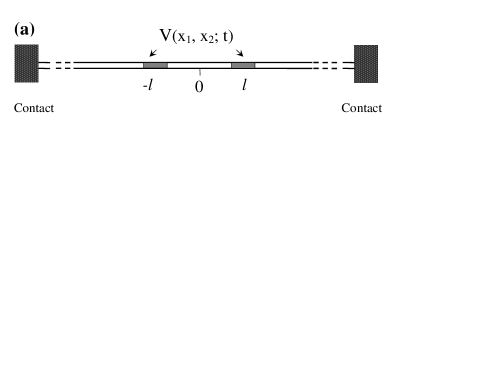
Figure 1: (a) Schematic figure of a one dimensional system in which the two-body interaction $V(x_{1},x_{2};t)$ acts when $x_{1}$ and $x_{2}$ are both within a finite interval near $-l$ or when both are within a finite interval near $l$.

III.2 Adiabatic Perturbation

The most commonly used description of quantum pumping employs the well-known Brouwer formula Brouwer-1 that derives directly from the Landauer-Buttiker formalism. Another common description uses Flouquet theory Floquet-Buttiker ; Floquet-Kim . Since those approaches rely upon single particle scattering matrix in 1D, not appropriate for describing interacting pairs, we have taken an a priori approach rooted in adiabatic perturbation as used by Thouless Thouless in his original paper on quantum pumping. That approach has been used in some recent papers nano-transport as well. This will merely constitute our point of departure, because we have the significant complication of interacting particles with pumping driven by the interaction, while the previous studies were derived in a single-particle picture.

The singlet current in Eq. (II.1) is defined in terms of a time-dependent singlet two particle state $\Psi_{\bar{k}}(\bar{x})$. Therefore the determination of the pumped current reduces to describing the evolution of this singlet state in the presence of a time-varying interaction $V(\bar{x},t)$

$$H=H_{0}+V(\bar{x},t)$$ (11)

in Eq. (II.2). Here, the free Hamiltonian $H_{0}$ is still time-independent and its two-body energy eigenstates are still of the form shown in Eq. (9) comprised of symmetric combinations of single particle eigenstates.

For an adiabatic process, the potential, or the two-particle interaction in our case, is assumed to vary slowly compared to the time spent by the particles in the region of the potential, i.e. the dwell time is much shorter than the time for variations in the potential Buttiker-Landauer . As a result, it is appropriate to insert the ansatz $\Psi_{\bar{k}}(\bar{x},t)=e^{-i\int dtE(\bar{k},t)/\hbar}\tilde{\Psi}_{\bar{k}}(\bar{x},t)$ into Eq. (II.2), we are left with

$$i\hbar\frac{\partial}{\partial t}\tilde{\Psi}_{\bar{k}}(\bar{x},t)=[H_{0}+V(\bar{x})-E(\bar{k},t)]\tilde{\Psi}_{\bar{k}}(\bar{x},t).$$ (12)

Henceforth we will drop the tilde symbol on $\tilde{\Psi}$; the phase $e^{-i\int dtE(\bar{k},t)/\hbar}$ that distinguishes $\Psi$ from $\tilde{\Psi}$ does not affect the current (II.1) in any case. To find a zeroth order solution, we neglect the time derivative and solve the instantaneous equation

$$[E(\bar{k},t)-H_{0}-V(\bar{x},t)]\Psi_{\bar{k}}^{t}(\bar{x}) = 0$$

where the time $t$ is simply a parameter. This equation on inversion becomes the Lippman-Schwinger equation, Eq (10), for the instantaneous scattering state $\Psi_{\bar{k}}^{t}(\bar{x})$. To find corrections, we evaluate the instantaneous Green’s function

$$[E-H_{0}-V(\bar{x},t)]G^{t}(\bar{x},\bar{x}^{\prime};E) = \delta(\bar{x}-\bar{x}^{\prime}),$$ (14)

and note that the exact solution to (12) is

$$\Psi_{\bar{k}}(\bar{x},t)=\Psi_{\bar{k}}^{t}(\bar{x})-i\hbar\int d\bar{x}^{\prime}G^{t}(\bar{x},\bar{x}^{\prime};E)\frac{\partial}{\partial t}\Psi_{\bar{k}}(\bar{x}^{\prime},t).$$ (15)

Iterating this equation, we can compute corrections to the zeroth order solution $\Psi_{\bar{k}}^{t}(\bar{x})$. To first order,

$$\Psi_{\bar{k}}(\bar{x},t) \simeq \Psi_{\bar{k}}^{t}(\bar{x})-i\hbar\int d\bar{x}^{\prime}G^{t}(\bar{x},\bar{x}^{\prime};E)\frac{\partial}{\partial t}\Psi_{\bar{k}}^{t}(\bar{x}^{\prime})$$ (16)

$$\equiv \Psi_{\bar{k}}^{t}(\bar{x})+\Delta\Psi_{\bar{k}}(\bar{x},t)$$

Higher orders are left out here because of the assumption of adiabaticity. Taking the derivatives of Eqs (III.2,14) with respect to time yields the following important identities for the time derivatives of the instantaneous functions

$$\dot{\Psi}_{\bar{k}}^{t}(\bar{x}) = \int d\bar{x}^{\prime}G^{t}(\bar{x},\bar{x}^{\prime};E)\dot{V}(\bar{x}^{\prime},t)\Psi_{\bar{k}}^{t}(\bar{x}^{\prime})$$ (17)

$$\dot{G}^{t}(\bar{x},\bar{x}^{\prime};E) = \int d\bar{x}^{\prime\prime}G^{t}(\bar{x},\bar{x}^{\prime};E)\dot{V}(\bar{x}^{\prime\prime},t)G^{t}(\bar{x}^{\prime\prime},\bar{x}^{\prime};E)$$

which allow us to write the second term in Eq.(16)(the term first order in the time derivative) as

$$\Delta\Psi_{\bar{k}}(\bar{x},t)=-i\hbar\int d\bar{x}^{\prime}G^{t}(\bar{x},\bar{x}^{\prime};E)\dot{\Psi}^{t}(\bar{x}^{\prime})$$

$$= -i\hbar\int d\bar{x}^{\prime}\int d\bar{x}^{\prime\prime}G^{t}(\bar{x},\bar{x}^{\prime};E)G^{t}(\bar{x}^{\prime},\bar{x}^{\prime\prime};E)\dot{V}(\vec{x}^{\prime\prime})\Psi^{t}(\vec{x}^{\prime\prime})$$

while the zeroeth order term is simply $\Psi^{t}_{\bar{k}}(\bar{x})$ determined by the Lippmann-Schwinger equation (10).

Henceforth, we sometimes simplify notation by writing $G(\bar{x},\bar{x}^{\prime})$ instead of $G^{t}(\bar{x},\bar{x}^{\prime};E)$.

III.3 Zeroth order: No Spontaneous Current

At the zeroth order in the time-dependence, at each instant the system is unaware of the fact that the potential is changing. Since there is no bias either, the current should vanish, because a non-vanishing current at this order would essentially be a spontaneous current, which is unphysical. In order to demonstrate that our definition of the singlet current passes this crucial test, we explicitly evaluate the current at the zeroth order in the time-derivative, which is given by

$$J_{0} = \frac{e\hbar}{m}\int dEf(E)\int dx_{2}\int\frac{dk_{1}}{2\pi}\int\frac{dk_{2}}{2\pi}$$

$$\times\delta\left({\textstyle\frac{\hbar^{2}k_{1}^{2}}{2m}+\frac{\hbar^{2}k_{2}^{2}}{2m}}-E\right){\rm Im}\left\{\Psi_{\bar{k}}^{t*}(\bar{x})\partial_{x_{1}}\Psi_{\bar{k}}^{t}(\bar{x})\right\}$$

Using the following identity for the free two particle Green’s function

$${\rm Im}\{G_{0}(\bar{x},\bar{x}^{\prime};E)\}=-\pi\int d\bar{k}\delta\left({\textstyle\frac{\hbar^{2}\bar{k}^{2}}{2m}}-E\right)\Phi_{\bar{k}}(\bar{x})\Phi_{\bar{k}}^{*}(\bar{x}^{\prime})$$ (20)

together with the Lippman-Schwinger Eq. (10) we can reduce the expression (III.3) to

$$J_{0} = \frac{-e\hbar}{\pi m}\int dEf(E)\int dx_{2}{\rm Im}\left[\partial_{x_{1}}{\rm Im}\{G_{0}(\bar{x},\bar{x}^{\prime})\}\right.$$ (21)

$$+\int d\bar{x}^{\prime\prime}\left\{\partial_{x_{1}}G(\bar{x};\bar{x}^{\prime\prime})\right\}V(\bar{x}^{\prime\prime}){\rm Im}\{G_{0}(\bar{x}^{\prime\prime},\bar{x})\}$$

$$+\int d\bar{x}^{\prime}\left.G^{*}(\bar{x};\bar{x}^{\prime})V(\bar{x}^{\prime})\partial_{x_{1}}{\rm Im}\{G_{0}(\bar{x},\bar{x}^{\prime})\}\right.$$

$$+\int d\bar{x}^{\prime}\int d\bar{x}^{\prime\prime}\left\{G^{*}(\bar{x};\bar{x}^{\prime})V(\bar{x}^{\prime})\right\}$$

$$\hskip 28.45274pt\left.\partial_{x_{1}}\left\{G(\bar{x};\bar{x}^{\prime\prime})V(\bar{x}^{\prime\prime}){\rm Im}\{G_{0}(\bar{x}^{\prime\prime},\bar{x}^{\prime})\right\}\right]$$

The first term vanishes immediately because it involves the imaginary part of a real number. Then after some manipulations where we use the Lippmann-Schwinger equation, the Dyson equation $G=G_{0}+G_{0}VG$, along with the reciprocity property of the Green’s functions, the expression for the current at the zeroeth order can be reduced to

$$J_{0} = \frac{e\hbar}{2\pi m}\int dE\ f(E)\int d\bar{x}^{\prime}\int d\bar{x}^{\prime\prime}V(\bar{x}^{\prime})V(\bar{x}^{\prime\prime})$$

$$\times\ {\rm Im}\left\{iG(\bar{x}^{\prime\prime};\bar{x}^{\prime})\int dx_{2}\left[G_{0}(\bar{x}^{\prime},\bar{x})\partial_{x_{1}}G_{0}(\bar{x};\bar{x}^{\prime\prime})\right]\right.$$

$$\ \ \ \ -\left.iG^{*}(\bar{x}^{\prime\prime};\bar{x}^{\prime})\int dx_{2}\left[G_{0}^{*}(\bar{x};\bar{x}^{\prime\prime})\partial_{x_{1}}G_{0}^{*}(\bar{x},\bar{x}^{\prime})\right]\right\}.$$

The kernel of the integral is of the form $F\times I_{GG}(x_{1},\bar{x}^{\prime},\bar{x}^{\prime\prime})$ evaluated in Eq. (74) in Appendix B (here $F=iG(x^{\prime},x^{\prime\prime};E)$). Such an integral was shown to vanish for $|x_{1}|>|x_{1}^{\prime}|,|x_{1}^{\prime\prime}|$. This applies here since the current is measured outside the region of interaction and the variables $x_{1}^{\prime}$ and $x_{1}^{\prime\prime}$ are associated with the localized interaction factors $V(\bar{x}^{\prime})$ and $V(\bar{x}^{\prime\prime})$. Therefore the net current at the zeroeth order vanishes, $J_{0}=0$ .

III.4 First order: Adiabatic Pumped Current

The pumped current to first adiabatic order is a bilinear form involving the zeroth order wavefunction $\Psi_{\bar{k}}^{t}(\bar{x})$ and the first order wavefunction correction $\Delta\Psi_{\bar{k}}(\bar{x},t)$ from Eq. (16):

$$J_{1}=\frac{e\hbar}{m}\int dEf(E)\int dx_{2}\int\frac{dk_{1}}{2\pi}\int\frac{dk_{2}}{2\pi}\ \delta\left({\textstyle\frac{\hbar^{2}k_{1}^{2}}{2m}+\frac{\hbar^{2}k_{2}^{2}}{2m}}-E\right)$$

$$\times{\rm Im}\left\{\Psi_{\bar{k}}^{t*}(\bar{x})\partial_{x_{1}}\Delta\Psi_{\bar{k}}(\bar{x},t)+\Delta\Psi_{\bar{k}}^{*}(\bar{x},t)\partial_{x_{1}}\Psi_{\bar{k}}^{t}(\bar{x})\right\}\hskip 5.69054pt$$ (23)

Using the identity in Eq. (20) and by multiple use of the Lippmann-Schwinger equation and the Dyson equation, in a straightforward but lengthy calculation, the above expression can be reduced to

$$J_{1} = -\frac{e\hbar^{2}}{2\pi m}\int dEf(E)\int d\bar{x}^{\prime}\int d\bar{x}^{\prime\prime}\dot{V}(\bar{x}^{\prime\prime})\int dx_{2}$$

$$\times \left[\left\{G^{*}(\bar{x}^{\prime\prime},\bar{x})-G(\bar{x}^{\prime\prime},\bar{x})\right\}\partial_{x_{1}}\left\{G(\bar{x},\bar{x}^{\prime})G(\bar{x}^{\prime}\bar{x}^{\prime\prime})\right\}\right.$$

$$- \left.\left\{G^{*}(\bar{x},\bar{x}^{\prime})G^{*}(\bar{x}^{\prime}\bar{x}^{\prime\prime})\right\}\partial_{x_{1}}\left\{G^{*}(\bar{x},\bar{x}^{\prime\prime})-G(\bar{x},\bar{x}^{\prime\prime})\right\}\right].$$

The identity $\int d\bar{x}^{\prime}G(\bar{x},\bar{x}^{\prime})G(\bar{x}^{\prime},\bar{x}^{\prime\prime})=-\partial_{E}G(\bar{x},\bar{x}^{\prime\prime})$, (Appendix A) then transforms this to

$$J_{1} = J_{1a}+J_{1b}$$

$$J_{1a} = \frac{\hbar^{2}}{2\pi m}\int dE\ f(E)\frac{\partial}{\partial E}\left[\int d\bar{x}^{\prime\prime}\dot{V}(\bar{x}^{\prime\prime})\int dx_{2}{\rm Im}\{G^{*}(\bar{x}^{\prime\prime},\bar{x};E)\partial_{x_{1}}G(\bar{x},\bar{x}^{\prime\prime};E)\}\right]$$

$$J_{1b} = \frac{\hbar^{2}}{2\pi m}\int dE\ f(E)\int d\bar{x}^{\prime}\int d\bar{x}^{\prime\prime}\dot{V}(\bar{x}^{\prime\prime}){\rm Im}\{G^{*}(\bar{x}^{\prime},\bar{x}^{\prime\prime};E)\int dx_{2}G^{*}(\bar{x},\bar{x}^{\prime};E)\partial_{x_{1}}G^{*}(\bar{x},\bar{x}^{\prime\prime};E)$$ (25)

$$\hskip 170.71652pt+G(\bar{x}^{\prime},\bar{x}^{\prime\prime};E)\int dx_{2}G(\bar{x}^{\prime\prime},\bar{x};E)\partial_{x_{1}}G(\bar{x},\bar{x}^{\prime};E)\}$$

We will now show that for any observation point $x_{1}$ greater than the region of non-vanishing $V$, the term $J_{1b}$ would not contribute in a periodically varying pumping cycle. We should first point out that the pair of terms in $J_{1b}$ are not complex conjugates, due to the assymmetry with respect to the exchange of $\bar{x}^{\prime}\leftrightarrow\bar{x}^{\prime\prime}$, so we cannot argue that taking the imaginary part makes it vanish. Using the Dyson equation we can make the following expansion

$${\rm Im}\left\{G^{*}(\bar{x}^{\prime},\bar{x}^{\prime\prime};E){\textstyle{\textstyle\int}}dx_{2}G^{*}(\bar{x},\bar{x}^{\prime};E)\partial_{x_{1}}G^{*}(\bar{x},\bar{x}^{\prime\prime};E)+G(\bar{x}^{\prime},\bar{x}^{\prime\prime};E){\textstyle\int}dx_{2}G(\bar{x}^{\prime\prime},\bar{x};E)\partial_{x_{1}}G(\bar{x},\bar{x}^{\prime};E)\right\}$$

$$= {\rm Im}\left\{G^{*}(\bar{x}^{\prime},\bar{x}^{\prime\prime}){\textstyle\int}dx_{2}G^{*}_{0}(\bar{x},\bar{x}^{\prime})\partial_{x_{1}}G^{*}_{0}(\bar{x},\bar{x}^{\prime\prime})+G(\bar{x}^{\prime},\bar{x}^{\prime\prime}){\textstyle\int}dx_{2}G_{0}(\bar{x},\bar{x}^{\prime\prime})\partial_{x_{1}}G_{0}(\bar{x},\bar{x}^{\prime})\right\}$$

$$+ {\textstyle\int}d\bar{y}\ {\rm Im}\left\{G^{*}(\bar{x}^{\prime},\bar{x}^{\prime\prime})V(\bar{y})G^{*}(\bar{y},\bar{x}^{\prime\prime}){\textstyle\int}dx_{2}G^{*}_{0}(\bar{x},\bar{x}^{\prime})\partial_{x_{1}}G^{*}_{0}(\bar{x},\bar{y})+G(\bar{x}^{\prime},\bar{x}^{\prime\prime})V(\bar{y})G(\bar{y},\bar{x}^{\prime\prime}){\textstyle\int}dx_{2}G_{0}(\bar{x},\bar{y})\partial_{x_{1}}G_{0}(\bar{x},\bar{x}^{\prime})\right\}$$

$$+ {\textstyle\int}d\bar{z}\ {\rm Im}\left\{G^{*}(\bar{x}^{\prime},\bar{x}^{\prime\prime})G^{*}(\bar{z},\bar{x}^{\prime})V(\bar{z}){\textstyle\int}dx_{2}G^{*}_{0}(\bar{x},\bar{z})\partial_{x_{1}}G^{*}_{0}(\bar{x},\bar{x}^{\prime\prime})+G(\bar{x}^{\prime},\bar{x}^{\prime\prime})V(\bar{z})G(\bar{z},\bar{x}^{\prime}){\textstyle\int}dx_{2}G_{0}(\bar{x},\bar{x}^{\prime\prime})\partial_{x_{1}}G_{0}(\bar{x},\bar{z})\right\}$$

$$+ {\textstyle\int}d\bar{z}{\textstyle\int}d\bar{y}\ {\rm Im}\ \left\{G^{*}(\bar{x}^{\prime},\bar{x}^{\prime\prime})\{V(\bar{y})G^{*}(\bar{y},\bar{x}^{\prime})V(\bar{z})G^{*}(\bar{z},\bar{x}^{\prime\prime})\}{\textstyle\int}dx_{2}G^{*}_{0}(\bar{x},\bar{y})\partial_{x_{1}}G^{*}_{0}(\bar{x},\bar{z})\right.$$ (26)

$$\left.\hskip 113.81102pt+G(\bar{x}^{\prime},\bar{x}^{\prime\prime})\{V(\bar{y})G(\bar{y},\bar{x}^{\prime\prime})V(\bar{z})G(\bar{z},\bar{x}^{\prime})\}{\textstyle\int}dx_{2}G_{0}(\bar{x},\bar{y})\partial_{x_{1}}G_{0}(\bar{x},\bar{z})\right\}$$

All four terms on the right hand side of the expression above involve integrals of the form $F\times I_{GG}(x_{1},\bar{x}^{\prime},\bar{x}^{\prime\prime})$ in Eq. (74) in  Appendix B, the function $F$ being different in each term. Using the properties of that integral in the Appendix we see easily that the last two terms would vanish for $x_{1}$ outside the interaction region. In fact if the observation point $|x_{1}|\rightarrow\infty$, which would guarantee $|x_{1}|>|x_{1}^{\prime}|$ , by the same argument the first two terms would be zero as well. However since the variable $x_{1}^{\prime}$ is not associated with any interaction factor $V$, in principle it is not bounded and we have to allow for $|x_{1}|<|x_{1}^{\prime}|$; in that case Eq (B.2) implies that for observation points outside the interaction region $|x_{1}|>|x_{1}^{\prime\prime}|$ , we can reduce the first two terms on the right hand side (which provide the only non-vanishing contributions) to

$$2\frac{m}{\hbar^{2}}\{\theta(x_{1}^{\prime}-x_{1})\theta(x_{1}-x_{1}^{\prime\prime})-\theta(x_{1}^{\prime\prime}-x_{1})\theta(x_{1}-x_{1}^{\prime})\}$$

$$\times{\rm Im}[G(\bar{x}^{\prime},\bar{x}^{\prime\prime})\{G_{0}(\bar{x}^{\prime},\bar{x}^{\prime\prime})+{\textstyle\int}d\bar{y}G_{0}(\bar{x}^{\prime},\bar{y})V(\bar{y})G(\bar{y},\bar{x}^{\prime\prime})\}]$$

$$=2\frac{m}{\hbar^{2}}{\rm Im}[G(\bar{x}^{\prime},\bar{x}^{\prime\prime})G(\bar{x}^{\prime},\bar{x}^{\prime\prime})]$$

$$\times\{\theta(x_{1}^{\prime}-x_{1})\theta(x_{1})-\theta(-x_{1})\theta(x_{1}-x_{1}^{\prime})\}$$ (27)

Inserting this into the second line of the expression for $J_{1b}$ in Eq (III.4) and using the identity in Eq (17) we get the following

$$J_{1b} = \frac{1}{\pi}\frac{\partial}{\partial_{t}}\int d\bar{x}^{\prime}\{\theta(x_{1}^{\prime}-x_{1})\theta(x_{1})-\theta(-x_{1})\theta(x_{1}-x_{1}^{\prime})\}$$

$$\times\int dE\ f(E){\rm Im}\{G(\vec{x}^{\prime},\vec{x}^{\prime};E)\}$$

$$= -\frac{\partial}{\partial_{t}}\int d\bar{x}^{\prime}\rho(\bar{x}^{\prime})$$

$$\times\{\theta(x_{1}^{\prime}-x_{1})\theta(x_{1})-\theta(-x_{1})\theta(x_{1}-x_{1}^{\prime})\}$$

In the last step we use the definition of the instantaneous two-dimensional density of states $\frac{1}{\pi}{\rm Im}\{G(\bar{x}^{\prime},\bar{x}^{\prime};E)\}=-\rho(\bar{x}^{\prime},E)$ and did the integral over energy to get the local density $\rho(\bar{x}^{\prime})$. As we see, this is a total time derivative that would vanish on integrating over a full period. In any case for an observation point $|x^{\prime}|\gg 0$ even without doing the time-integral, this term can be made negligible, and actually in the single particle picture used to describe charge pumping, the equivalent of this term is identically zero since the observation point is taken to be asymptotically far from the region of interaction. Thus we can now write a compact expression for the net contribution to the adiabatic pumped singlet current to first order for periodically varying two particle interaction,

$$J_{1}(t) = \frac{e\hbar^{2}}{2\pi m}\int dE\ f(E)\frac{\partial}{\partial E}\left[\int d\bar{x}^{\prime}\dot{V}(\bar{x}^{\prime})\int dx_{2}{\rm Im}\{G^{*}(\bar{x}^{\prime},\bar{x};E)\partial_{x_{1}}G(\bar{x},\bar{x}^{\prime};E)\}\right].$$ (29)

IV Validity for the non-interacting case: Charge pumping

Our result has the advantage that it also describes adiabatic quantum pumping where the independent particle description is assumed. We simply interpret the functions as single-particle objects, i.e. the green’s functions are single particle green functions, $G(\bar{x}^{\prime},\bar{x}^{\prime\prime};E)\rightarrow g(x^{\prime},x^{\prime\prime};E)$, and we then do not have the integral over $x_{2}$, so that

$$J(t)=\frac{e\hbar^{2}}{2\pi m}\int dE\ f(E)\frac{\partial}{\partial E}$$ (30)

$$\hskip 28.45274pt\times\left[\int dx^{\prime}\dot{V}(x^{\prime}){\rm Im}\{g^{*}(x^{\prime},x;E)\partial_{x}g(x,x^{\prime};E)\}\right]$$

Noting that the single particle Green’s function has the asymptotic form

$$g(x,x^{\prime\prime};E)=\frac{m}{ik\hbar^{2}}e^{ikx}\psi^{*}(x^{\prime})$$ (31)

where $k=\sqrt{2mE/\hbar^{2}}$, one obtains

$$J(x,t)=\frac{em}{2\pi\hbar^{2}}\int dE\ f(E)\frac{\partial}{\partial E}\left\{\frac{1}{k}\langle\psi|\dot{V}|\psi\rangle\right\}$$ (32)

which agrees with the expression in Ref.[nano-transport, ] on noting that in that paper the states are normalized by $\sqrt{k}$. That expression in turn has been shown to be equivalent to the Brouwer formula Brouwer-1 .

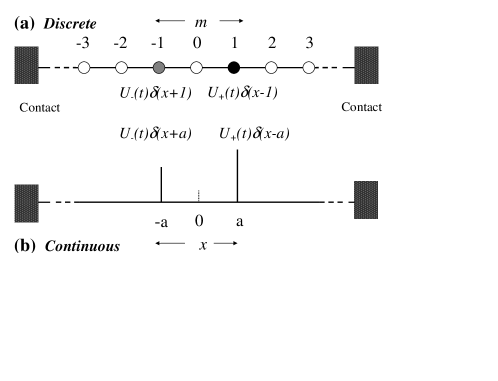
Figure 2: (a) A discrete model for a singlet pump comprising of a chain of quantum dots where the interaction between a singlet pair is non-vanishing only when both particles are together at one of the two shaded dots. (b) The continuum version of the same model where the pair interaction is non-zero only at the two points $x=\pm a$ indicated by spikes. The strengths of the two-particle interaction at the two sites are $U_{\pm}(t)$ which are the time-varying parameters. At any instant the two parameters can be of different magnitude indicated by different shades in the discrete model and different heights of the spikes in the continuum model (the short dotted line is simply a marker for the origin $x=0$).

V Physical model for a Singlet Pump: A lattice of quantum dots

In theoretical studies of quantum pumping, a turnstile model Levinson-turnstile has been used, wherein delta function potentials exist at two points in a 1D system. The cyclic variation of the strength of the potentials serves as the pumping cycle. The region between the two spikes can be interpreted as a scattering region, such as a quantum dot, and the strength of the potentials a measure of the barriers segregating the scattering region from the rest of the system (e.g. the leads). We can adapt the turnstile model, proposing a singlet pump in which delta function external potentials acting at the two points are replaced with the electron-electron interaction acting only at those points. In a continuum of positions, this model of extremely localized interactions seems somewhat unrealistic. However, in a 1D tight-binding lattice, we would have interactions at two lattice sites, which seems physically reasonable and appropriate for the application of our results. Physically such a lattice model could be implemented, for instance, by a chain of quantum dots where precise voltage controls produce only time-varying interaction between the members of an electron pair when both particles occupy one of two specific dots. A schematic of the model is shown in Fig. 2.

Formally the expressions in the discrete case are identical with those of the continuum case, as we have verified explicitly Das-PRL : The Green’s functions in the continuum case need only be reinterpreted as discrete Green’s functions and spatial integrals need only be replaced by spatial sums. Since the general derivation in this paper has been in a continuum model, we will derive the results for the turnstile model also in a continuum form.

The interaction is

$$V(\bar{x},t)=U_{-}(t)\delta(\bar{x}+\bar{a})+U_{+}(t)\delta(\bar{x}-\bar{a})$$ (33)

where $\pm\bar{a}\equiv\pm\{a,a\}$. The strength of the delta functions $U_{-}$ and $U_{+}$ are the two time-dependent pumping parameters. The instantaneous pumped singlet current in Eq (29) then becomes

$$J_{S}(t) = \frac{e\hbar^{2}}{2\pi m}\int dEf(E)\sum_{\bar{y}=\pm\bar{a}}\dot{U}_{\pm}(t)$$ (34)

$$\times\partial_{E}{\rm Im}\left[\int dx_{2}G^{*}(\bar{x},\bar{y})\partial_{x_{1}}G(\bar{x},\bar{y})\right]$$

The full instantaneous Green’s function for this system can be written compactly as

$$G(\bar{x},\bar{y})=G_{0}(\bar{x},\bar{y})+F_{-}(\bar{y})G_{0}(\bar{x},-\bar{a})+F_{+}(\bar{y})G_{0}(\bar{x},\bar{a})$$

with the coefficients being

$$F_{\pm}(\bar{y})=\left[\frac{T_{\pm}G_{0}(\pm\bar{a},\bar{y})+T_{\pm}T_{\mp}G_{0}(2\bar{a})G_{0}(\mp\bar{a},\bar{y})}{1-T_{\mp}T_{\pm}G_{0}(2\bar{a})G_{0}(2\bar{a})}\right].$$ (35)

We have introduced the T-matrix for a single Hubbard interaction (a single term in Eq. (33)),

$$T_{\pm}(t)=[U_{\pm}^{-1}(t)+G_{0}(0)]^{-1}.$$ (36)

We have also introduced a shorthand for the free Green’s functions: Since the free Green’s functions depend only on the absolute difference of the coordinates, $G_{0}(\bar{x},\bar{y})=G_{0}(|\bar{x}-\bar{y}|)$, we define $G_{0}(2\bar{a})=G_{0}(\bar{a},-\bar{a})=G_{0}(-\bar{a},\bar{a})$ and $G_{0}(0)=G_{0}(\bar{a},\bar{a})=G_{0}(-\bar{a},-\bar{a})$. Using the expansion Eq. (V) we can evaluate the coordinate integrals in Eq (34) to be

$$\frac{\hbar^{2}}{m}\int dx_{2}G^{*}(\bar{x},\pm\bar{a})\frac{\partial}{\partial_{x_{1}}}G(\bar{x},\pm\bar{a})=$$ (37)

$$-{\rm Im}\{G_{0}(0)\}\left[1+[F_{\pm}(\vec{a})+F_{\pm}^{*}(\vec{a})]+|F_{\mp}(\vec{a})|^{2}+|F_{\mp}(\vec{a})|^{2}\right]$$

$$-{\rm Im}\{F_{\mp}(\vec{a})G_{0R}(2a)-F_{\mp}^{*}(\vec{a})G_{0R}^{*}(2a)\}$$

$$-{\rm Im}\{F_{\pm}^{*}(\vec{a})F_{\mp}(\vec{a})G_{0R}(2a)-F_{\mp}^{*}(\vec{a})F_{\pm}(\vec{a})G_{0R}^{*}(2a)\}$$

In order to obtain this form we used the expansion Eq (V) above to reduce the above integral to a sum of integrals of the form shown in Eqs. (57)and (60) considered in the Appendix B. Then we used their respected evaluated forms given in Eqs. (61) and (B.1). What is noteworthy is that the expressions depend on $G_{0R}(2a)$, the regular part of the two-particle Green’s function which has no singularity. This is discussed in the Appendix in Eq. (56) After carrying through a lengthy but straightforward set of algebraic manipulations, of the above expression, we insert the result into Eq (34) to get the following expression for the singlets pumped in a single cycle of period $\tau$

$$Q_{S}(\tau)=\frac{-e}{2\pi}\int_{0}^{\tau}dt\int dEf(E)\frac{\partial}{\partial E}\sum_{\pm}\dot{U}_{\pm}(t)\frac{|T_{\pm}(t)|^{2}\left[{\rm Im}\{G_{0}(0)\}(1+|T_{\mp}(t)G_{0}(2\bar{a})|^{2})\pm 2{\rm Im}\{T_{\mp}(t)G_{0}(2\bar{a})G_{0R}^{\pm}(2\bar{a})\}\right]}{U_{\pm}(t)^{2}|1-T_{\mp}(t)T_{\pm}(t)G_{0}(2\bar{a})G_{0}(2\bar{a})|^{2}}.$$ (38)

where $G_{0R}^{+}(2\bar{a})=G_{0R}(2\bar{a})$ and $G_{0R}^{-}(2\bar{a})=G_{0R}^{*}(2\bar{a})$. Thus in order to evaluate the current we only need to evaluate the free two-particle lattice Green’s function, for only two specific arguments $G_{0}(0)=G_{0}(\bar{a},\bar{a};E)$ and $G_{0}(2\bar{a})=G_{0}(\bar{a},-\bar{a};E)$. Exact analytical forms exist for the lattice Green’s functions, $G_{0}$, in terms of elliptic integrals Economou .

As mentioned above the expression for the discrete lattice is identical to this with the replacement of the Green’s functions by their discrete equivalents $G_{0}(0)\rightarrow G_{0}(\bar{m},\bar{m};E)$ and $G_{0}(2\bar{a})\rightarrow G_{0}(\bar{m},-\bar{m};E)$ where $\pm m$ correspond to the lattice sites where the time varying interaction occurs. In Fig. 2(a), we take $m=1$. The effect of changing the value of $m$ on the number singlet pairs pumped per cycle was presented in an earlier paper Das-PRL .

VI Characteristics of a Quantum dot for time-varying interaction

While the physical model comprising of a chain of quantum dots as presented above yields a measurable singlet current in theory, the actual experimental implementation requires a feasibility study involving realistic quantum dots. We will now suggest a specific configuration for an experimentally realizable quantum dot to tailor it for singlet pumping. In the rest of the paper, we will establish that the characteristics of our proposed configuration will allow the variation and manipulations to satisfy the requirements of a singlet pump.

To maintain close contact with experiments, we specifically consider a cylindrically symmetric GaAs/Al_xGa_1-xAs quantum dot used in experiments reported in Ref. Ashoori, . To adapt the dot for singlet pumping, we propose a single modification: instead of being one single disk, the top gate needs to be made of an inner disk of radius $R_{in}$ and a concentric outer annulus with inner and outer radii $R_{in}$ and $R_{out}$, so that the voltages $V_{in}$ and $V_{out}$ on the two pieces can be controlled independently. This provides two independent parameters for manipulating the shape and depth of the lateral potential. A schematic cut-away view is shown in Fig. 3, in the original experiment (a) and with our proposed modification (b).

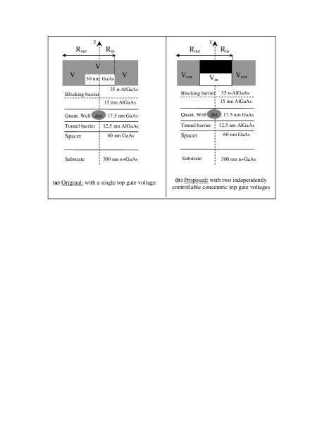
Figure 3: (a) Schematic figure of the quantum dot used in Refs. [Ashoori, ] and [Bednarek, ]. Here $V$ is the potential energy at the top gate. (b) Our proposed modification of that structure with two concentric metal gates, with independently controllable voltages; $V_{in}$ is the net potential energy of an electron at the top edge of the blocking barrier ($V_{in}=-e\times\Phi_{in}$, where $\Phi_{in}$ is the voltage) right below the inner gate (darker shade). Likewise $V_{out}$ is the potential energy of an electron at the base of the outer gate (lighter shade).

Along the direction of the z-axis (Fig. 3), electron confinement is provided by the difference in conduction band edge energies between GaAs and Al_xGa_1-xAs. The result is a quantum well of width 17.5 nm in the middle GaAs layer. Lateral confinement within that GaAs layer is due to the inhomogeneous electric potential generated by the top gate. In the original setup, a 30 nm thick GaAs cylindrical cap over the center of the dot created that inhomogeneity, while in our modified version, the different voltages on the inner and outer discs both play a role in the lateral confinement. The inhomogeneity is such that the potential energy of an electron V ($=-e\times\Phi$ where $\Phi$ is the gate voltage) is lower near the axis of the dot so that electrons are attracted to the region under the inner disc or cap.

We determine the potential profile within the dot by numerically solving the Poisson equation

$$(\nabla_{R}^{2}+\partial_{z}^{2})V=\left\{\begin{array}[]{cr}0&0<z<105\ {\rm nm}\\ (-e)\times-\frac{n_{D}e}{K\epsilon_{0}}&105<z<140\ {\rm nm}\end{array}\right.$$ (41)

applying the methods and parameters used in Ref. Bednarek, to match experimental observed capacitance spectroscopy peaks of Ref. Ashoori, . Here, $z$ is measured from the top of the substrate, so that the region $105\ {\rm nm}<z<140\ {\rm nm}$ is the charged blocking barrier. In the Poisson equation, $K=12.85$ is the dielectric constant for undoped GaAs, and the charge density in the blocking barrier is taken to be $n_{D}=4.62\times 10^{17}$ cm^-3. We take the Fermi energy of the bottom electrode as the energy reference, and specify $V_{in}$ and $V_{out}$ at the top surface of the cylinder. Thus, at $z=140$ nm, $V_{in}$ is taken to be a positive constant potential energy in the inner disk of radius $R_{in}$ and $V_{out}$ is a positive constant potential energy on the outer disc between $R_{in}$ and $R_{out}$ (to create electron confinement we must have $V_{in}<V_{out}$). The potentials are defined to be those at the edge of the blocking barrier, $z=140$ nm, so that $V_{in}$ and $V_{out}$ include the Schottky potential of about $0.65$ eV at the metal gate semiconductor interface, as well as the drop due to the GaAs cap under the inner disk. The boundary condition on the curved outer surface of the cylindrical dot is set by assuming a large value of $R_{out}$, so that the electric field is essentially parallel to the curved surface and aligned along the z-direction. We solve the 1D Poisson equation in the z-direction to determine the potential profile on this outer surface at $r=R_{out}$

$$V(R_{out},z)=\left\{\begin{array}[]{cr}B_{1}z+B_{2}&z<105\ {\rm nm}\\ +\frac{n_{D}e^{2}}{K\epsilon_{0}}\frac{z^{2}}{2}+A_{1}z+A_{2}&z>105\ {\rm nm}\end{array}\right..$$ (44)

Applying the boundary conditions at the top ($V=V_{out}$) and bottom surface ($V=0$) and matching solutions at the bottom edge of the blocking barrier layer at $z=105$ nm determines the constants $A_{1}=(V_{out}-9.9684)/140\ {\rm eV/nm},B_{1}=(V_{out}-0.3987)/140\ {\rm eV/nm},A_{2}=3.5886\ {\rm eV},{\rm and}\ B_{2}=0$.

With the value of the potential on the boundary determined, the full 2D Poisson equation in $r,z$ is solved using FISHPACK FORTRAN routines for the solution of separable elliptic partial differential equations FISHPACK . Figure 4 plots the shape of the potential without the 0.22 eV conduction band offset of the AlGaAs; we took $R_{in}=120$ nm and $R_{out}=400$ nm. Fig. 5(a) shows the computed z-profile along the cylinder axis at $R=0$ nm now with the 0.22 eV AlGaAs offset included; this shows that the region where electrons are trapped resembles a finite square well along the z-axis. Fig. 5(b) shows the computed profile, in the middle of the finite square well ($z=90$ nm), in the radial direction. The solid line is a parabolic fit, which shows clearly that in the radial direction the trapped electrons feel a harmonic oscillator potential.

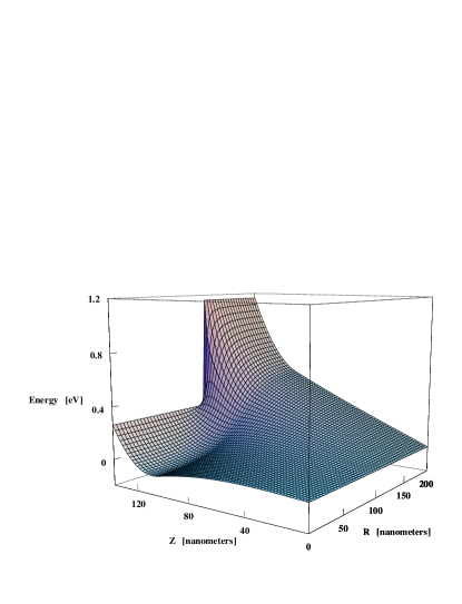
Figure 4: Potential energy of an electron in the structure depicted in Fig. 3(b), without the 0.22 eV offsets due to the AlGaAs layers.

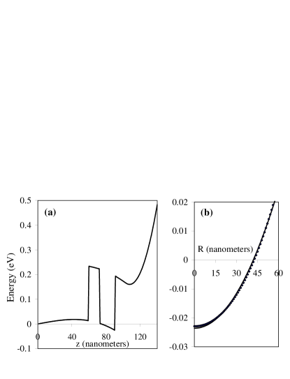
Figure 5: Radial and axial profiles of the potential along lines passing through the center of the quantum dot obtained from the solution of the Poisson equation for the structure depicted in Fig. 3(b). (a) Axial (z) profile along the cylinder axes (R=0) including the 0.22 eV band offset (b) Radial profile at z=90 nm where the potential is the lowest; the black dots correspond to the solution of the Poisson equation, and the continuous line is the parabolic fit.

VII An Electron-pair in the modified quantum dot

The problem of two electrons in a quantum dot has been analyzed in detail in the literature. As we see from Fig. 5, the potential in our quantum dot is well approximated by a finite square well in the z-direction and a harmonic oscillator in the radial direction. The effective Hamiltonian operator for two electrons is then

$$\hat{H}=-\frac{\hbar^{2}}{2m^{*}}\left[\nabla^{2}_{r1}+\partial_{z1}^{2}+\nabla^{2}_{r2}+\partial_{z2}^{2}\right]+V_{sq.well}$$

$$+\frac{e^{2}/4\pi\epsilon_{0}K}{(r_{1}-r_{2})^{2}+(z_{1}-z_{2})^{2}}+\frac{1}{2}m^{*}\omega^{2}(r_{1}^{2}+r_{2}^{2})$$ (45)

In the numerical estimates that follow, we neglect the $z-$dependance in the Coulomb interaction in order to separate the radial and axial directions in the Schrodinger equation. Quantitatively, the neglect of this term in the denominator of the Coulomb interaction will cause a slight overestimate of the Coulomb interaction energy, an effect that can be diminished if the dot is significantly narrower along the z-axis than in the radial direction. However, qualitatively this approximation makes no difference for the demonstration of quantum pumping feasibility.

The total energy of an electron in the dot can now be separated into two parts $E=E_{z}+E_{R}$, an axial quantum well energy $E_{Z}$ which is well approximated by a finite square well and a transverse energy $E_{R}$ that can be well approximated using a harmonic oscillator.

VII.1 Axial energy, $E_{z}$

The size of the quantum well is $L=17.5$ nm. and the height is given by $U=|U_{0}|+0.22$ eV, where $0.22$eV is the band offset between GaAs and Al_xGa_1-xAs and $U_{0}$ is the depth of the well below the Fermi energy of the bottom lead, our reference energy. For an infinite well of the same width we get: $E_{z}^{\infty}=\frac{2\hbar^{2}}{m^{*}L^{2}}\times\left(\frac{\pi}{2}\right)^{2}=18.31{\rm meV}$ taking $m^{*}=0.067m$ for undoped GaAs. For a finite square well, the ground state energy is determined by

$$E_{z}=\frac{2\hbar^{2}x^{2}}{m^{*}L^{2}}=(7.43{\rm meV})\times x^{2};\hskip 5.69046ptx\tan(x) = \sqrt{P^{2}-x^{2}}$$

with $P^{2}=134.8\times U{\rm(in\ eV)}$ where $U$ is the well depth. We found that as $U$ varies over the range (0.22, 0.26)  eV, $E_{z}$ remains in the range (13.0, 13.4)meV. Since it turns out that $U_{0}$ changes by less than $0.01$eV when we vary the parameters $V_{out}$ and $V_{in}$, the value of $E_{Z}$, which is defined relative to the bottom of the well, changes by less than $\sim 1\%$. Therefore, in our calculations, the variation of $E_{Z}$ relative to the bottom of the well can be neglected. As Fig. 5(a) shows, the bottom of the well is not completely flat, varying from $0.22$eV to $|U_{o}|+0.22$eV. However, for the same reason, this slope has little effect on the constancy of $E_{Z}$.

VII.2 Radial energy, $E_{R}$

The transverse or radial Hamiltonian can be separated into center-of-mass (R) and relative coordinates (r) Zhu

$$H_{com} = -\frac{1}{2}\nabla^{2}_{R}+\frac{1}{2}\gamma^{2}R^{2}$$

$$H_{rel} = -2\nabla^{2}_{r}+\frac{1}{8}\gamma^{2}r^{2}+\frac{2}{r}$$ (46)

where energies are scaled in Rydbergs $R_{D}=\frac{\hbar^{2}}{2m^{*}a_{D}^{2}}$ and the length scale is $a_{D}=\hbar^{2}(4\pi\epsilon_{0}K)/(m^{*}e^{2})$ and $\gamma=2(a_{D}/l_{0})^{2}$ where $l_{0}=\sqrt{\hbar/m^{*}\omega}$ is the oscillator length. In these units, the harmonic oscillator energy spacing, $\hbar\omega$, is given by $R_{D}\gamma$. Excluding the Coulomb interaction the solutions are those for a 2-dimensional harmonic oscillator with circular symmetry with energy

$$E_{R}-E_{int}=(2N+1+|M|)\gamma+(2n+1+|m|)\gamma.$$ (47)

The parity of the spatial wavefunction is determined by the relative coordinate quantum number $m$. For $m=0$, the spatial wavefunction is even under particle change ($r\rightarrow-r$), so the state must have an antisymmetric spin wavefunction, a singlet. For $m=1$ the spatial wavefunction is odd under particle interchange, so the state must have a symmetric spin wavefunction, a triplet. We conclude that the lowest energy states are the singlet with $(N,M,n,m)=(0,0,0,0)$ and the triplet with $(N,M,n,m)=(0,0,0,1)$. These have energies $2\hbar\omega$ and $3\hbar\omega$ respectively without including the Coulomb interaction energy $E_{int}$.

The interaction energy $E_{int}$ has been calculated for 2D circular quantum wells in the literature Zhu ; McKinney for values of $\gamma\sim 0.1-1$. We use those results for $E_{int}$ to determine the total radial energy $E_{R}$.

VIII Experimental Feasibility of Pumping Entangled Electrons

VIII.1 Desired scenario for singlet pumping

We would like to vary the top gate potential energies $V_{in}$ and $V_{out}$ in such a way that the shape of the lateral confining potential changes with the following constraints:

(i) At all times, the singlet state is energetically accessible, but the triplet state is too high in energy to be occupied.

(ii) The energy of a single electron in the dot with respect to the Fermi energy $E_{F}=0$ of the bottom electrode stays constant and far off resonance with $E_{F}$. This suppresses single electron tunneling, which depends strongly on including the resonant region in the pumping cycle Levinson-turnstile .

(iii) There is significant variation of the Coulomb interaction between the two electrons: the singlet energy can be varied appreciably to permit pumping of pairs.

We present numerically computed results for two sample configurations of the dot corresponding to different specific values of the top gate potential energies $V_{in}$ and $V_{out}$ which satisfy the above criteria. These two configurations could serve as points within a cyclic variation of the top gate potential energies.

The lowest energy state spin singlet (with quantum numbers $(N,M,n,m)=(0,0,0,0)$) and spin triplet (with quantum numbers $(N,M,n,m)=(0,0,0,1)$) have total energies:

$$1s:\hskip 14.22636ptE^{(S)}(\omega)=2U_{0}+2E_{z}+2\hbar\omega+E_{int}^{(S)}(\omega)$$

$$2p:\hskip 14.22636ptE^{(T)}(\omega)=2U_{0}+2E_{z}+3\hbar\omega+E_{int}^{(T)}(\omega)$$ (48)

In order to satisfy condition (i) we look for values of $\omega$ such that the total triplet energy lies above the Fermi level i.e. the reference energy in our calculations, while the $E^{(S)}$ lies below:

$$E^{(S)}(\omega)<0\hskip 28.45274ptE^{(T)}(\omega)>0$$ (49)

In order to satisfy condition (ii) to maintain the single particle energy levels fixed with respect to the Fermi level, we have to simultaneously ensure that in any two configurations (1 and 2), we have:

$$\hbar\omega_{1}+U_{0}^{(1)}+E_{z}=\hbar\omega_{2}+U_{0}^{(2)}+E_{z},$$ (50)

$$\Rightarrow\ \hbar\omega_{1}-\hbar\omega_{2}=U_{0}^{(2)}-U_{0}^{(1)}.$$

Table 1: Summary of numerically computed parameters for two specific configurations of the potential profile of the proposed quantum dot, that would satisfy the requirements of singlet pumping. The two configurations would be part of a continuous and cyclic variation of the potential profile of the dot.

		$Configuration\ 1$	$Configuration\ 2$
	$V_{out}$	$1158.1\ meV$	$950.6\ meV$
	$V_{in}$	$263.1\ meV$	$301.2\ meV$
	$l_{0}=\sqrt{\hbar/m^{*}\omega}$	$14.35\ nm$	$15.55\ nm$
	$\hbar\omega$	$5.5\ meV$	$4.7meV$
	$U_{0}$	$-22.9\ meV$	$-22.1\ meV$
	$E_{Z}$	$13.2\ meV$	$13.2\ meV$
Single Electron level	$U_{0}+E_{Z}+\hbar\omega$	$-4.2\ meV$	$-4.2\ meV$
Singlet interaction energy	$E_{int}^{(S)}$	$7.3\ meV$	$6.6\ meV$
Triplet interaction energy	$E_{int}^{(T)}$	$4.6\ meV$	$4.2meV$
	$E_{int}^{(T)}-E_{int}^{(S)}$	$-2.7\ meV$	$-2.4\ meV$
Radial Singlet energy	$E_{R}^{(S)}$	$18.4\ meV$	$16.0meV$
Radial Triplet energy	$E_{R}^{(T)}$	$21.2\ meV$	$18.3\ meV$
	$E_{R}^{(T)}-E_{R}^{(S)}$	$2.8\ meV$	$2.3\ meV$
Total Singlet energy	$2U_{0}+2E_{z}+E_{R}^{(S)}$	$-0.5\ meV$	$-0.9\ meV$
Total Triplet energy	$2U_{0}+2E_{z}+E_{R}^{(T)}$	$+0.9\ meV$	$+0.25\ meV$

Figure 6: (a) Radial profiles through the lowest potential region of the dot for two distinct set of top gate potential energies: continuous line $\rightarrow(V_{out},V_{in})=(1158.1\ {\rm meV},263.1\ {\rm meV})$ and dotted line $\rightarrow(V_{out},V_{in})=(950.6\ {\rm meV},301.2\ {\rm meV})$. They correspond to the two configurations described in Table I. (b) Expanded view of the lowest energy region. The shift $U_{0}$ between the two configurations is $\hbar\omega_{1}-\hbar\omega_{2}$, keeping the single particle ground state energy unchanged.

VIII.2 Experimental parameters for singlet pumping

We take the dimensions of our quantum dot to be similar to those of Ref. Ashoori, , except that our dot has a slightly smaller radius of $120$ nm for the inner top gate while estimates Bednarek found that in the experiment the radius of the GaAs cap was about $200$ nm.

We explicitly identify two sample locations in parameter space that satisfy all of our conditions. (To find a complete pumping path through parameter space is straightforward since one has two parameters $V_{out}$ and $V_{in}$ and only one precise quantitative constraint (ii) above). Say the two sample locations have radial oscillator energies $\hbar\omega=5.5$ meV and $\hbar\omega=4.7$ eV (corresponding to $\gamma=1$ and $\gamma=0.85$ respectively). Then the well depths must compensate such that the single electron energy (50) remains constant. For example, the locations could satisfy $U_{0}=-22.9$ meV and $U_{0}=-22.1$ meV so that the single electron energy is held at $-4.2$ meV, constant and strongly off resonance with the Fermi energy. At these values of $\hbar\omega$ and $U_{0}$, the quantum dot geometry is such that the interaction energies Zhu for singlets are $7.3$ meV and $6.6$ meV respectively and for triplets $4.6$ meV and $4.2$ meV, respectively. Then equation (48) implies that the total energies for the singlets are $-0.5$ meV and $-0.9$ meV for the two locations in parameter space while the total energies of the triplets are $0.9$ meV and $0.25$ meV respectively. Thus, the singlet states are energetically accessible while the triplet states are not.

Our simulation shows that the two configurations are realized in the dot at $(V_{out},V_{in})=(1158.1{\rm meV},263.1{\rm meV})$ and $(V_{out},V_{in})=(950.6{\rm meV},301.2{\rm meV})$, from our numerical computation, which can be rounded off to the appropriate significant figures. Figure 6(a) shows the radial profile in the dot for the two configurations. Configuration 1 has a higher difference between $V_{in}$ and $V_{out}$, leading to a larger value of $\omega$ and causing tighter lateral confinement. Configuration 2 has a lower difference between $V_{in}$ and $V_{out}$ leading to smaller value of $\omega$. However, because $V_{in}$ is higher than in configuration 1, the well is not as deep. This can be clearly seen in Fig. 6(b) where the profiles for the two configurations cross due to the compensating effects of increased $\omega$ and lowered $U_{0}$.

Table I summarizes the results of our simulation. Energetically the singlets are accessible in both configurations, while triplets are inaccessible (point (i) above). The energy of the single electron level in the dot is fixed at $-4.2{\rm meV}$ significantly off-resonant with $E_{F}=0$ (point (ii) above). The variation of the Coulomb interaction is about $11\%$ between the two singlet configurations (point (iii) above).

IX Conclusions

In this paper we address several issues related to developing a quantum singlet pump. We will conclude by providing a summary of our main results. We have considered the problem of applying the mechanism of adiabatic quantum pumping to generate a flow of singlet pairs of electrons, while suppressing the flow of triplets and uncorrelated single particles. The first challenge was to find the appropriate theoretical description. We first identified an appropriate definition of the current for singlet pairs in analogy with the current of a stream of uncorrelated electrons, by using the reduced two-particle density matrix. We then showed how in the presence of two-body interactions, the evolution of the many electron system can be effectively described by the evolution of a two-particle state particularly when the interaction is spatially localized. We confirmed that our definition of current gives a non-zero current in the absence of bias or time variation. We then wrote an adiabatic perturbation expansion for the time varying two particle states, where the rate of change of the interaction $\partial V/\partial t$ is assumed slow compared to the time scale of the dwell time of the particles in the interaction region. Using the assumption of adiabaticity, we computed the pumped current to first order in the time derivative (or equivalently the frequency of the time-varying interaction). The interaction is assumed to affect only singlets and is non-vanishing only in a finite region, but otherwise completely general. By using several identities and relations for two particle Green’s function, that we present in the appendices, we reduced the expression for the current to a compact and relatively simple form involving only the instantaneous two particle Green’s functions. The current is seen to have an additional transient term which we show vanishes identically for a complete cycle, the term being a total time derivative.

Having established a general but simple expression for the pumped singlet current due to the action of a time-varying local two body interaction, we apply it to a specific model. We consider a lattice, where the interaction acts and varies in time only at two of the sites; the interaction acts only when both particles are localized on the same site, while the two sites are sufficiently separated that interaction among an electron at one site with one at the other can be neglected. If the sites are well localized in space, the effect of the interaction on triplets is automatically suppressed due to vanishing or at least substantial suppression of the triplet spatial wavefunction at each of the two sites due to the Pauli principle. We computed the singlet current for the model as an exact analytical expression, which has been confirmed to have the same form for discrete and continuous models.

Finally we show that this model can be implemented using a chain of quantum dots. We take the design specifications of a quantum dot that had been fabricated and studied in the lab and propose one minor modification that would introduce two concentric top gates with independently controllable voltages, something that can be achieved without much difficulty with the methods of fabrication available currently. We computed the potential profile of such a dot with available experimental parameters and computed the energy of two electrons in such a dot. We showed that by varying the two gate voltages, (i) significant singlet current can be generated (ii) triplets can be made energetically inaccessible for states in the dot, and therefore affected much less by the variation of the interaction (iii) the single particle states can be maintained at the same energy and far off-resonance, thereby suppressing current of uncorrelated single electrons. Thus in effect such a dot can be used in a chain to implement our model for generation of a measurable singlet current.

Appendix A Greens functions: Representations and Identities

The Green’s function for the potential-free time-independent Schrodinger equation is defined by

$$[E+\textstyle{\frac{\hbar^{2}}{2m}}\nabla^{2}]G_{0}(\bar{x}^{\prime},\bar{x}^{\prime\prime};E)=\delta(\bar{x}^{\prime}-\bar{x}^{\prime\prime})$$ (51)

where $\bar{x}\equiv\{x_{1},x_{2},\cdots,x_{n}\}$ denotes the spatial degrees of freedom, the total energy $E$ shared among them is assumed real, and the subscript in $G_{0}$ indicates the absence of any potential. The degrees of freedom have equivalent interpretations as $n$ spatial dimensions or as coordinates of $n$ individual particles in one dimension. We study interacting particles in 1D, but we use ‘n-particle’ or ‘$n$D’ interchangeably in referring to the Green’s functions. The retarded and advanced Green’s functions will be denoted using superscripts $G^{+}$ and $G^{-}$. When the Green’s functions obey $G_{0}^{+}(\bar{x}^{\prime},\bar{x}^{\prime\prime};E)=[G_{0}^{-}(\bar{x}^{\prime},\bar{x}^{\prime\prime};E)]^{*}$, we leave out the superscripts, $G^{+}\equiv G$ and $G^{-}\equiv G^{*}$.

Our interest being in two body interactions we only need single particle (or 1D) and two particle (or 2D) Green’s functions. The uppercase $G(\bar{x}^{\prime},\bar{x}^{\prime\prime};E)$ will be reserved for 2D Green’s function with $\bar{x}\equiv\{x_{1},x_{2}\}$, and 1D Green’s functions will be distinguished by using lowercase $g_{0}(x,x^{\prime};E)$. Single-particle eigenstates are likewise denoted by lowercase $\phi_{k}(x)$; expansion in such eigenstates readily establishes the following useful identities:

$$\int_{-\infty}^{\infty}dx\phi_{k}^{*}(x)g_{0}(x,x^{\prime};E) = \frac{\phi_{k}^{*}(x^{\prime})}{E-E_{k}+i\eta}$$ (52)

$$\int_{-\infty}^{\infty}d\epsilon\frac{g_{0}(x^{\prime},x^{\prime\prime};E-\epsilon)}{\epsilon-E_{p}+i\eta} = -2i\pi g_{0}(x^{\prime},x^{\prime\prime};E-E_{p})$$

$$\int_{-\infty}^{\infty}d\epsilon\frac{g_{0}(x^{\prime},x^{\prime\prime};E-\epsilon)}{\epsilon-E_{p}-i\eta} = 0$$

$$\int_{-\infty}^{\infty}dxg_{0}^{*}(x,x^{\prime};E_{1})g_{0}(x,x^{\prime\prime};E_{2})=\hskip 79.6678pt$$

$$\frac{g_{0}^{*}(x^{\prime\prime},x^{\prime};E_{1})-g_{0}(x^{\prime},x^{\prime\prime};E_{2})}{E_{2}-E_{1}+i\eta}$$

$$\int_{-\infty}^{\infty}dxg_{0}(x,x^{\prime};E_{1})g_{0}(x,x^{\prime\prime};E_{2})=\hskip 82.51282pt$$

$$\frac{g_{0}(x^{\prime\prime},x^{\prime};E_{1})-g_{0}(x^{\prime},x^{\prime\prime};E_{2})}{E_{2}-E_{1}}\stackrel{{\scriptstyle E_{2}\rightarrow E_{1}}}{{\rightarrow}}-\frac{\partial}{\partial_{E_{1}}}g(x^{\prime},x^{\prime\prime};E_{1})$$

For scattering problems the appropriate eigenstates are plane waves which in 1D are $\phi_{k}(x)=e^{ikx}$; they provide a coordinate representation for the free 1D Green’s function for real energies $E$

$$g_{0}^{\pm}(x^{\prime},x^{\prime\prime};E)=\int_{-\infty}^{\infty}\frac{dk}{2\pi}\frac{e^{ik(x^{\prime}-x^{\prime\prime})}}{E-(\hbar^{2}k^{2}/2m)\pm i\eta}$$

$$= \mp\frac{i\theta(E)e^{\pm i\sqrt{\frac{2m}{\hbar^{2}}E}|x^{\prime}-x^{\prime\prime}|}}{\frac{\hbar^{2}}{m}\sqrt{2mE/\hbar^{2}}}-\frac{\theta(-E)e^{-\sqrt{\frac{2m}{\hbar^{2}}|E|}|x^{\prime}-x^{\prime\prime}|}}{\frac{\hbar^{2}}{m}\sqrt{2m|E|/\hbar^{2}}}$$

The difference of the retarded and the advanced Green’s functions gives the two-point correlation function

$$\rho(x^{\prime},x^{\prime\prime};E) = \frac{1}{-2\pi i}\left[g_{0}^{+}(x^{\prime},x^{\prime\prime};E)-g_{0}^{-}(x^{\prime\prime},x^{\prime};E)\right]$$

$$= \theta(E)\int_{-\infty}^{\infty}\frac{dk}{2\pi}\delta(E-(\hbar^{2}k^{2}/2m))e^{ik(x^{\prime}-x^{\prime\prime})}$$

Performing the momentum integral demonstrates consistency with the definition of $g_{0}^{\pm}$. In the case of equal coordinate arguments a different contour integral is involved, but the end result agrees with simply setting $x^{\prime}=x^{\prime\prime}$ in the above expressions; $\rho(x^{\prime},x^{\prime};E)$ defines the one-dimensional density of states.

The 2D free Green’s function can be written in terms of the 1D Green’s functions

$$G_{0}^{\pm}(\bar{x}^{\prime}\bar{x}^{\prime\prime};E) =$$

$$\frac{\pm i}{2\pi}\int_{-\infty}^{\infty}d\epsilon g_{0}^{\pm}(x_{1}^{\prime},x_{1}^{\prime\prime};E-\epsilon)g_{0}^{\pm}(x_{2}^{\prime},x_{2}^{\prime\prime};\epsilon)$$

Using an eigenfunction expansion in Cartesian coordinates and integrating out one momentum component gives

$$G_{0}^{\pm}(\bar{x}^{\prime}\bar{x}^{\prime\prime};E)=$$ (56)

$$\mp i\int_{0}^{\sqrt{\frac{2mE}{\hbar^{2}}}}\frac{dk}{2\pi}\frac{2\cos[k(x_{2}^{\prime}-x_{2}^{\prime\prime})]e^{\pm i\sqrt{2mE/\hbar^{2}-k^{2}}|x_{1}^{\prime}-x_{1}^{\prime\prime}|}}{\frac{\hbar^{2}}{m}\sqrt{2mE/\hbar^{2}-k^{2}}}$$

$$-\int_{\sqrt{\frac{2mE}{\hbar^{2}}}}^{\infty}\frac{dk}{2\pi}\frac{2\cos[k(x_{2}^{\prime}-x_{2}^{\prime\prime})]e^{-\sqrt{k^{2}-2mE/\hbar^{2}}|x_{1}^{\prime}-x_{1}^{\prime\prime}|}}{\frac{\hbar^{2}}{m}\sqrt{k^{2}-2mE/\hbar^{2}}}.$$

The first term has both real and imaginary parts and is always regular ($R$) as a function of the coordinate arguments, while second term is always real and is singular ($S$) when $\bar{x}^{\prime}=\bar{x}^{\prime\prime}$; so we name the two terms $G_{0R}^{\pm}(\bar{x}^{\prime}\bar{x}^{\prime\prime};E)$ and $G_{0S}^{\pm}(\bar{x}^{\prime}\bar{x}^{\prime\prime};E)$ respectively.

Appendix B Integrals used in computing current

We will apply the results of the preceding appendix to evaluate the generic expressions involving two particle or 2D Green’s functions required in computing current. The 2D Green’s functions below are at energy $E$, not explicitly shown for the sake of compact notation.

B.1 Integral with conjugate Green’s functions

We encounter expressions involving a pair of conjugate 2D Green’s functions when computing the current:

$$I_{G^{*}G}(\bar{x}^{\prime},\bar{x}^{\prime\prime})=\int_{-\infty}^{\infty}dx_{2}G_{0}^{*}(\bar{x},\bar{x}^{\prime})\frac{\partial}{\partial x_{1}}G_{0}(\bar{x},\bar{x}^{\prime\prime})$$ (57)

By expressing the 2D Green’s functions above in terms of 1D Green’s functions as in Eq. (A), and then using the identities in Eq. (52) we can reduce it to the form

$$I_{G^{*}G}(x_{1},\bar{x}^{\prime},\bar{x}^{\prime\prime}) = \frac{i}{2\pi}\int_{-\infty}^{\infty}d\epsilon[g(x_{2}^{\prime},x_{2}^{\prime\prime};\epsilon)-g^{*}(x_{2}^{\prime},x_{2}^{\prime\prime};\epsilon)]$$ (58)

$$\times g^{*}(x_{1},x_{1}^{\prime};E-\epsilon)\frac{\partial}{\partial x_{1}}g(x_{1},x_{1}^{\prime\prime};E-\epsilon).$$

Inserting the expressions for 1D Green’s functions from Eqs. (A) and (A) leads to an explicit functional form that is piecewise continuous, in which the free variable $x_{1}$ determines the boundaries of continuity; thus for the exterior region $|x_{1}|>|x_{1}^{\prime}|,|x_{1}^{\prime\prime}|$, which is relevant to us, the expression is

$$I_{G^{*}G}(x_{1},\bar{x}^{\prime},\bar{x}^{\prime\prime})=$$ (59)

$$\pm\left[i\int_{0}^{\sqrt{\frac{2mE}{\hbar^{2}}}}\frac{dk}{2\pi}\frac{2\cos[k(x_{2}^{\prime}-x_{2}^{\prime\prime})]e^{\pm i\sqrt{\frac{2m}{\hbar^{2}}E-k^{2}}(x_{1}^{\prime}-x_{1}^{\prime\prime})}}{\frac{\hbar^{4}}{m^{2}}\sqrt{2mE/\hbar^{2}-k^{2}}}\right.$$

$$\left.-\int_{\sqrt{\frac{2mE}{\hbar^{2}}}}^{\infty}\frac{dk}{2\pi}\frac{2\cos[k(x_{2}^{\prime}-x_{2}^{\prime\prime})]e^{-\sqrt{k^{2}-\frac{2m}{\hbar^{2}}E}|2x_{1}-(x_{1}^{\prime}+x_{1}^{\prime\prime})|}}{\frac{\hbar^{4}}{m^{2}}\sqrt{k^{2}-2mE/\hbar^{2}}}\right]$$

where the $+$ sign applies for $x_{1}>x_{1}^{\prime},x_{1}^{\prime\prime}$ and the $-$ sign for $x_{1}<x_{1}^{\prime},x_{1}^{\prime\prime}$. We can exploit the similarity of this expression with $G_{0}^{\pm}(\bar{x}^{\prime}\bar{x}^{\prime\prime})$ in Eq. (56) because we always encounter it in the functional combination

$$F\times I_{G^{*}G}(x_{1},\bar{x}^{\prime},\bar{x}^{\prime\prime})=\hskip 113.81102pt$$ (60)

$${\rm Im}\left\{F\int_{-\infty}^{\infty}dx_{2}G_{0}^{*}(\bar{x},\bar{x}^{\prime})\frac{\partial}{\partial x_{1}}G_{0}(\bar{x},\bar{x}^{\prime\prime})\right.$$

$$\left.+F^{*}\int_{-\infty}^{\infty}dx_{2}G_{0}^{*}(\bar{x},\bar{x}^{\prime\prime})\frac{\partial}{\partial x_{1}}G_{0}(\bar{x},\bar{x}^{\prime})\right\}$$

where $F$ is a complex-valued function and $\bar{x}^{\prime}\leftrightarrow\bar{x}^{\prime\prime}$ are exchanged between the two terms; the second term in Eqs. (59), being (i) manifestly real and (ii) unaffected by the exchange $\bar{x}^{\prime}\leftrightarrow\bar{x}^{\prime\prime}$, would not contribute to Eq. (60). Therefore, in this particular combination the integrals can be replaced by $G_{0R}^{\pm}(\bar{x}^{\prime}\bar{x}^{\prime\prime})$. We need to note that the exponential in Eq. (56) contains the absolute difference of the coordinate arguments while Eq. (59) does not; this in effect determines the choice of $G_{0R}^{\pm}$ depending on whether $x^{\prime}>x^{\prime\prime}$ or $x^{\prime}<x^{\prime\prime}$:

$${\rm For}\ x_{1}>x_{1}^{\prime},x_{1}^{\prime\prime},\hskip 8.53581ptF\times I_{G^{*}G}(\bar{x}^{\prime},\bar{x}^{\prime\prime})=\hskip 65.44142pt$$ (61)

$$\frac{m}{\hbar^{2}}{\rm Im}\left\{-[FG_{0R}(\bar{x}^{\prime},\bar{x}^{\prime\prime})-F^{*}G_{0R}^{*}(\bar{x}^{\prime},\bar{x}^{\prime\prime})]\theta(x_{1}^{\prime}-x_{1}^{\prime\prime})\right.$$

$$\left.\hskip 11.38109pt+[FG_{0R}^{*}(\bar{x}^{\prime},\bar{x}^{\prime\prime})-F^{*}G_{0R}(\bar{x}^{\prime},\bar{x}^{\prime\prime})]\theta(x_{1}^{\prime\prime}-x_{1}^{\prime})]\right\}$$

$${\rm For}\ x_{1}<x_{1}^{\prime},x_{1}^{\prime\prime},\hskip 8.53581ptF\times I_{G^{*}G}(\bar{x}^{\prime},\bar{x}^{\prime\prime})=\hskip 65.44142pt$$

$$\frac{m}{\hbar^{2}}{\rm Im}\left\{-[FG_{0R}^{*}(\bar{x}^{\prime},\bar{x}^{\prime\prime})-F^{*}G_{0R}(\bar{x}^{\prime},\bar{x}^{\prime\prime})]\theta(x_{1}^{\prime}-x_{1}^{\prime\prime})]\right.$$

$$\left.\hskip 11.38109pt+[FG_{0R}(\bar{x}^{\prime},\bar{x}^{\prime\prime})-F^{*}G_{0R}^{*}(\bar{x}^{\prime},\bar{x}^{\prime\prime})]\theta(x_{1}^{\prime\prime}-x_{1}^{\prime})]\right\}$$

It is also useful to note that the imaginary part satisfies

$${\rm Im}\left\{I_{G^{*}G}(\bar{x}^{\prime},\bar{x}^{\prime\prime})\right\} = \left\{\begin{array}[]{lr}-\frac{m}{\hbar^{2}}{\rm Im}\{G_{0}(\bar{x}^{\prime},\bar{x}^{\prime\prime})\}&x_{1}>x_{1}^{\prime},x_{1}^{\prime\prime}\\ +\frac{m}{\hbar^{2}}{\rm Im}\{G_{0}(\bar{x}^{\prime},\bar{x}^{\prime\prime})\}&x_{1}<x_{1}^{\prime},x_{1}^{\prime\prime}\end{array}\right.$$ (64)

which helps simplify the case $\bar{x}^{\prime}=\bar{x}^{\prime\prime}$, when the first terms in both Eqs. (59) and (56) become imaginary

$$F\times I_{G^{*}G}(x_{1},\bar{x}^{\prime},\bar{x}^{\prime})\hskip 113.81102pt$$

$$=\left\{\begin{array}[]{lr}-\frac{m}{\hbar^{2}}{\rm Im}\{G_{0}(\bar{x}^{\prime},\bar{x}^{\prime})\}{\rm Re}(F)&x_{1}>x_{1}^{\prime}\\ +\frac{m}{\hbar^{2}}{\rm Im}\{G_{0}(\bar{x}^{\prime},\bar{x}^{\prime})\}{\rm Re}(F)&x_{1}<x_{1}^{\prime}\end{array}\right..$$ (67)

B.2 Integral with like Green’s functions

We also encounter expressions with a pair of similar 2D Green’s functions

$$I_{GG}(x_{1},\bar{x}^{\prime},\bar{x}^{\prime\prime})=\int_{-\infty}^{\infty}dx_{2}G_{0}(\bar{x},\bar{x}^{\prime})\frac{\partial}{\partial x_{1}}G_{0}(\bar{x},\bar{x}^{\prime\prime})$$ (68)

which, by using Eq. (A) and the identities in Eq. (52), can be reduced to the form

$$=\frac{i}{2\pi}\int_{-\infty}^{\infty}d\epsilon g(x_{2}^{\prime},x_{2}^{\prime\prime};\epsilon)g(x_{1},x_{1}^{\prime};E-\epsilon)$$

$$\times\frac{\partial}{\partial x_{1}}g(x_{1},x_{1}^{\prime\prime};E-\epsilon)$$ (69)

Then the expressions for the 1D Green’s functions in Eq. (A) provide explicit functional forms which, as in the previous case, depends on the value of $x_{1}$. For the exterior region $|x_{1}|>|x_{1}^{\prime}|,|x_{1}^{\prime\prime}|$ this is

$$I_{GG}(x_{1},\bar{x}^{\prime},\bar{x}^{\prime\prime}) = \pm\frac{i}{2\pi}\int_{-\infty}^{\infty}\!\!d\epsilon g_{\epsilon}(x_{2}^{\prime},x_{2}^{\prime\prime})$$

$$\left[\frac{e^{i\sqrt{2m(E-\epsilon)/\hbar^{2}}|2x_{1}-(x_{1}^{\prime}+x_{1}^{\prime\prime})|}}{i\frac{\hbar^{4}}{m^{2}}\sqrt{2m(E-\epsilon)/\hbar^{2}}}\theta(E-\epsilon)\right.$$

$$\left.-\frac{e^{-\sqrt{2m(\epsilon-E)/\hbar^{2}}|2x_{1}-(x_{1}^{\prime}+x_{1}^{\prime\prime})|}}{\frac{\hbar^{4}}{m^{2}}\sqrt{2m(\epsilon-E)/\hbar^{2}}}\theta(\epsilon-E)\right]$$

where the $+$ sign applies for $x_{1}>x_{1}^{\prime},x_{1}^{\prime\prime}$ and the $-$ sign for $x_{1}<x_{1}^{\prime},x_{1}^{\prime\prime}$. This integral is also of interest for interior region when $|x_{1}|$ is between $|x_{1}^{\prime}|$ and $|x_{1}^{\prime\prime}|$:

$$I_{GG}(x_{1},\bar{x}^{\prime},\bar{x}^{\prime\prime})=\left\{\begin{array}[]{lr}+\frac{m}{\hbar^{2}}G_{0}(\bar{x}^{\prime},\bar{x}^{\prime\prime})&x_{1}^{\prime}>x_{1}>x_{1}^{\prime\prime}\\ -\frac{m}{\hbar^{2}}G_{0}(\bar{x}^{\prime},\bar{x}^{\prime\prime})&x_{1}^{\prime\prime}>x_{1}>x_{1}^{\prime}\end{array}\right.$$ (73)

The following combination is relevant

$$F\times I_{GG}(x_{1},\bar{x}^{\prime},\bar{x}^{\prime\prime})=\hskip 85.35826pt$$ (74)

$${\rm Im}\left\{F\int_{-\infty}^{\infty}dx_{2}G_{0}(\bar{x},\bar{x}^{\prime})\frac{\partial}{\partial x_{1}}G_{0}(\bar{x},\bar{x}^{\prime\prime})\right.$$

$$\left.+F^{*}\int_{-\infty}^{\infty}dx_{2}G_{0}^{*}(\bar{x},\bar{x}^{\prime\prime})\frac{\partial}{\partial x_{1}}G_{0}^{*}(\bar{x},\bar{x}^{\prime})\right\}.$$

For the exterior region $I_{GG}(x_{1},\bar{x}^{\prime},\bar{x}^{\prime\prime})$ is invariant under exchange of coordinate arguments, so the expression above vanishes, $F\times I_{GG}(x_{1},\bar{x}^{\prime},\bar{x}^{\prime\prime})=0$, for the exterior region $|x_{1}|>|x_{1}^{\prime}|,|x_{1}^{\prime\prime}|$. In the interior region $I_{GG}(x_{1},\bar{x}^{\prime},\bar{x}^{\prime\prime})$ simply changes sign under such an exchange, so that for

$$F\times I_{GG}(\bar{x}^{\prime},\bar{x}^{\prime\prime})=\pm\frac{m}{\hbar^{2}}{\rm Im}\left\{FG_{0}(\bar{x}^{\prime},\bar{x}^{\prime\prime})-c.c.\right\}$$

$$=\left\{\begin{array}[]{lr}+2\frac{m}{\hbar^{2}}{\rm Im}\left\{FG_{0}(\bar{x}^{\prime},\bar{x}^{\prime\prime})\right\},&x_{1}^{\prime}>x_{1}>x_{1}^{\prime\prime}\\ -2\frac{m}{\hbar^{2}}{\rm Im}\left\{FG_{0}(\bar{x}^{\prime},\bar{x}^{\prime\prime})\right\},&x_{1}^{\prime\prime}>x_{1}>x_{1}^{\prime}\end{array}\right.$$ (76)

Appendix C An Effective Two Particle State for the Many body system

As soon as we consider pair interaction, in principle, we have to allow for interaction between all possible pairs in the system. In this Appendix we reduce a full many body system with pair interaction to an effective description in terms of a pair of interacting particles both moving in the background of the interaction field due to all the other electrons in the system. This allows us to describe the pumping of singlets in terms of the evolution of a singlet wavefunction very much like the pumping of individual electrons by a single particle state.

Using the composite notation for position and introduced in Sec. II, $X=(x,\sigma)$, the Heisenberg equation of motion of a Fermion creation operator with the Hamiltonian (II.2) is

$$i\hbar\partial_{t}\hat{\psi}^{\dagger}(X,t)=h(x)\hat{\psi}^{\dagger}(X,t)\hskip 85.35826pt$$

$$+\int dX^{\prime}\hat{\psi}^{\dagger}(X,t)\hat{\psi}^{\dagger}(X^{\prime},t)V(x,x^{\prime})\hat{\psi}(X^{\prime},t).$$ (78)

Consider $\langle E_{0},N|\hat{\psi}^{\dagger}(X_{1},t)\hat{\psi}^{\dagger}(X_{2},t)|E_{2},N-2\rangle$, a matrix element where $|E_{0},N\rangle$ is the N particle ground state of the system, and $|E_{2},N-2\rangle$ is an energy eigenstate with $N-2$ particles. Using Eq. (78), we find that the equation of motion of this matrix element is

$$i\hbar\partial_{t}\langle E_{0},N|\hat{\psi}^{\dagger}(X_{1},t)\hat{\psi}^{\dagger}(X_{2},t)|E_{2},N-2\rangle=(h(x_{1})+h(x_{2}))\langle E_{0},N|\hat{\psi}^{\dagger}(X_{1},t)\hat{\psi}^{\dagger}(X_{2},t)|E_{2},N-2\rangle$$

$$\hskip 56.9055pt+\int dX^{\prime}V(x_{1},x^{\prime})\langle E_{0},N|\hat{\psi}^{\dagger}(X_{1},t)\hat{\psi}^{\dagger}(X^{\prime},t)\hat{\psi}(X^{\prime},t)\hat{\psi}^{\dagger}(X_{2},t)|E_{2},N-2\rangle$$

$$\hskip 56.9055pt+\int dX^{\prime}V(x_{2},x^{\prime})\langle E_{0},N|\hat{\psi}^{\dagger}(X_{1},t)\hat{\psi}^{\dagger}(X_{2},t)\hat{\psi}^{\dagger}(X^{\prime},t)\hat{\psi}(X^{\prime},t)|E_{2},N-2\rangle$$ (79)

Since both $|E_{0},N\rangle$ and $|E_{2},N-2\rangle$ are energy eigenstates, we can replace $i\hbar\partial_{t}\rightarrow E=E_{2}-E_{0}$ on the left hand side of the above equations. Furthermore,

$$\hat{\psi}^{\dagger}(X^{\prime},t)\hat{\psi}(X^{\prime},t)\hat{\psi}^{\dagger}(X_{2},t)$$ (80)

$$= \delta(X^{\prime}-X_{2})\hat{\psi}^{\dagger}(X^{\prime},t)+\hat{\psi}^{\dagger}(X_{2},t)\hat{\psi}^{\dagger}(X^{\prime},t)\hat{\psi}(X^{\prime},t)$$

due to the Fermion commutation relations; here we denoted $\delta(X^{\prime}-X_{2})\equiv\delta_{\sigma^{\prime},\sigma_{2}}\delta(r^{\prime}-r_{2})$. Making a mean-field approximation, with the density of background electrons at $X^{\prime}$ defined by, $n(X^{\prime},t)=\langle E_{0},N-2|\hat{\psi}^{\dagger}(X^{\prime},t)\hat{\psi}(X^{\prime},t)|E_{0},N-2\rangle$, we define the two particle state

$$\Psi_{E}(X_{1},X_{2},t)\!=\!\langle E_{0},N|\hat{\psi}^{\dagger}\!(X_{1},t)\hat{\psi}^{\dagger}\!(X_{2},t)|E_{2},N\!-\!2\rangle\ \$$ (81)

and bring (79) into the form

$$E\Psi_{E}(X_{1},X_{2},t)$$

$$= [h(x_{1})+h(x_{2})+V(x_{1},x_{2})]\Psi_{E}(X_{1},X_{2},t)$$

$$+\int dX^{\prime}[V(x_{1},x^{\prime})+V(x_{2},x^{\prime})]n(X^{\prime},t)\Psi_{E}(X_{1},X_{2},t)$$

The last line gives the mean-field influence of the rest of the electrons with the particular pair of electrons at $X_{1}$ and $X_{2}$. We can include this in the one body potential that each particle experiences: $h(x)+\int dX^{\prime}V(x,x^{\prime})n(X^{\prime},t)\rightarrow h(x)$. Since the two-body interaction $V$ does not affect spin, we can factorize out the spin part of the wave function. Considering specifically the singlet subspace and by introducing the parametrization in terms of the single particle momentum labels $k_{1},k_{2}$ we are led to Eq (II.2).

References

• (1) L. P. Kouwenhoven, A. T. Johnson, N. C. van der Vaart, C. J. P. M. Harmans, and C. T. Foxon, Phys. Rev. Lett. 67, 1626 (1991).
• (2) H. Pothier, P. Lafarge, C. Urbina, D. Esteve, M. H. Devoret, Europhys. Lett. 17, 249 (1992).
• (3) M. Switkes, C. M. Marcus, K. Campman, and A. C. Gossard, Science 283, 1905 (1999).
• (4) E. M. Höhberger, A. Lorke, W. Wegscheider, and M. Bichler, Appl. Phys. Lett. 78, 2905 (2001).
• (5) S. K. Watson, R. M. Potok, C. M. Marcus, and V. Umansky, Phys. Rev. Lett. 91, 258301 (2003).
• (6) L. DiCarlo, C. M. Marcus, and J. S. Harris, Phys. Rev. Lett. 91, 246804 (2003).
• (7) M R Buitelaar, P J Leek, V I Talyanskii, C G Smith, D Anderson, G A C Jones, J Wei and D H Cobden, Semincond. Sci. Technol.21, S69 (2006)
• (8) B. Kaestner et al. cond-mat/0707.0993 (2007).
• (9) P. W. Brouwer, Phys. Rev. B 58, R10 135 (1998).
• (10) K. K. Das, S. Kim, and A. Mizel, Phys. Rev. Lett. 97, 096602 (2006); K. K. Das, S. Kim, and A. Mizel, Bull. Am. Phys. Soc. 49, 218 (2004).
• (11) S. Kim, K. K. Das, and A. Mizel, Phys. Rev. B 73, 075308 (2006).
• (12) I. L. Aleiner, B. L. Altshuler, and A. Kamenev, Phys. Rev. B 62, 10373 (2000).
• (13) B. L. Altshuler and L. I. Glazman, Science 283, 1864 (1999).
• (14) E. R. Mucciolo, C. Chamon, and C. M. Marcus, Phys. Rev. Lett. 89, 146802 (2002).
• (15) Y. Levinson, O. Entin-Wohlman, and P. Wölfle, Physica A 302, 335 (2001).
• (16) O. Entin-Wohlman, A. Aharony, and Y. Levinson, Phys. Rev. B 65, 195411 (2002).
• (17) X. Hu and S. Das Sarma,Phys. Rev. B 69, 115312 (2004).
• (18) M. Moskalets and M. Büttiker, Phys. Rev. B 66, 205320 (2002).
• (19) S. W. Kim, Phys. Rev. B 66, 235304 (2002).
• (20) T. Aono, Phys. Rev. B 67, 155303 (2003).
• (21) M. Blaauboer and C. M. L. Fricot, Phys. Rev. B 71, 041303(R) (2005).
• (22) P. Samuelsson and M. Büttiker, Phys. Rev. B 71, 245317 (2005).
• (23) C. W. J. Beenakker, M. Titov, and B. Trauzettel, Phys. Rev. Lett. 94, 186804 (2005).
• (24) D. J. Thouless, Phys. Rev. B 27, 6083 (1983).
• (25) J. E. Avron, A. Elgart, G. M. Graf, and L. Sadun, Jour. Stat. Phys. 116, 425 (2004).
• (26) P. Sharma and C. Chamon, Phys. Rev. Lett. 87, 096401 (2001).
• (27) R. Citro, N. Andrei, Q. Niu Phys. Rev. B 68 165312 (2003).
• (28) D. Bohm, Quantum Theory, (Prentice-Hall, New Jersey, 1951).
• (29) M. A. Nielsen and I. L. Chuang, Quantum Computation and Quantum Information, (Cambridge, New York, 2000).
• (30) M. Büttiker and R. Landauer, Phys. Rev. Lett. 49, 1739 (1982).
• (31) E. N. Economou, Green’s Functions in Quantum Physics, (Springer-Verlag, Berlin, 1979).
• (32) R.C. Ashoori, H. L. Stormer, J. S. Weiner, L. N. Pfeiffer, S. J. Pearton, K. W. Baldwin, and K. W. West, Phys. Rev. Lett. 68, 3088 (1992).
• (33) S. Bednarek, B. Szafran, K. Lis, and J. Adamowski, Phys. Rev. B 68, 155333 (2003).
• (34) FISHPACK: a package of fortran subprograms for the solution of separable elliptic partial differential equations, J. Adams, P. Swarzrauber, and R. Sweet, (version 4.0 , June 1999).
• (35) J. L. Zhu, Z. Q. Li, J. Z. Yu, K. Ohno, and Y. Kawazoe, Phys. Rev. B 55, 15819 (1997).
• (36) B. A. McKinney and D. K. Watson, Phys. Rev. B 61, 4958 (2000).