Comparison of Boltzmann Kinetics with Quantum Dynamics
for a Chiral Yukawa Model Far From Equilibrium

Abstract

Boltzmann equations are often used to describe the non-equilibrium time-evolution of many-body systems in particle physics. Prominent examples are the computation of the baryon asymmetry of the universe and the evolution of the quark-gluon plasma after a relativistic heavy ion collision. However, Boltzmann equations are only a classical approximation of the quantum thermalization process, which is described by so-called Kadanoff-Baym equations. This raises the question how reliable Boltzmann equations are as approximations to the complete Kadanoff-Baym equations. Therefore, we present in this article a detailed comparison of Boltzmann and Kadanoff-Baym equations in the framework of a chirally invariant Yukawa-type quantum field theory including fermions and scalars. The obtained numerical results reveal significant differences between both types of equations. Apart from quantitative differences, on a qualitative level the late-time universality respected by Kadanoff-Baym equations is severely restricted in the case of Boltzmann equations. Furthermore, Kadanoff-Baym equations strongly separate the time scales between kinetic and chemical equilibration. In contrast to this standard Boltzmann equations cannot describe the process of quantum-chemical equilibration, and consequently also cannot feature the above separation of time scales.

I Introduction

This article is an extension of our previous studies Lindner:2005kv , where we performed a detailed comparison of Boltzmann and Kadanoff-Baym equations in the framework of a real scalar $\Phi^{4}$ quantum field theory. The motivation for these studies is a better understanding of processes like leptogenesis or preheating in the early universe Sakharov:1967dj ; Fukugita:1986hr ; Buchmuller:2000nd ; Berges:2002cz , or the evolution of the quark-gluon plasma after relativistic heavy-ion collisions Arsene:2004fa ; Back:2004je ; Adams:2005dq ; Adcox:2004mh . All these phenomena require the description of many-particle systems out of thermal equilibrium. The standard means to deal with this non-equilibrium situation are Boltzmann equations. However, it is well known that (classical) Boltzmann equations suffer from several shortcomings as compared to their quantum mechanical generalizations, so-called Kadanoff-Baym equations. This motivates a comparison of Boltzmann and Kadanoff-Baym equations in order to assess the reliability of quantitative predictions based on standard Boltzmann techniques. In the present work we generalize our previous results to the case of a chirally invariant Yukawa-type quantum field theory coupling fermions with scalars. More precisely, we consider a globally $SU(2)\times SU(2)\times U(1)$ symmetric quantum field theory, which offers two interpretations for the particle content: On one hand, in the context of leptogenesis one might think of a single generation of leptons and a Higgs bidoublet Deshpande:1990ip . On the other hand, this theory is equivalent to the linear $\sigma$-model Schwinger:1957em ; polkinghorne1958a ; Gell-Mann:1960np , which can be used to describe low-energy quark-meson dynamics in two-flavor QCD. In any case, this work can be regarded as a further step to approach more realistic theories, which can be used to describe the phenomena motivating our studies.

What are the shortcomings of Boltzmann equations? Originally, Boltzmann equations have been designed for the description of the non-equilibrium time-evolution of dilute gases of classical particles. As such, their range of validity must be scrutinized once quantum effects become relevant. This is certainly the case for elementary particles playing the central role in phenomena like leptogenesis or the quark-gluon plasma. As already indicated above, the quantum dynamics of such systems is described by so-called Kadanoff-Baym equations. Employing a sequence of approximations, Boltzmann equations can be derived from Kadanoff-Baym equations baymKadanoff1962a ; Danielewicz:1982kk ; Ivanov:1999tj ; Knoll:2001jx ; Blaizot:2001nr . However, it is important to note that these approximations might be neither justifiable nor controllable, and sometimes even inconsistent. After all, standard Boltzmann equations take only on-shell processes into account, feature spurious constants of motion, and introduce irreversibility by implying the assumption of molecular chaos (“Stoßzahlansatz”) landauLifshitzVolume10 ; balescu1975a ; deGroot1980a ; kreuzer1981a . In contrast to this, Kadanoff-Baym equations are time-reversal invariant and take memory and off-shell effects into account Berges:2000ur ; kohler1995a ; kohler1996a ; Aarts:2001qa . Therefore, one should perform a detailed comparison of Boltzmann and Kadanoff-Baym equations Danielewicz:1982ca ; kohler1995a ; kohler1996a ; Morawetz:1998em ; Juchem:2003bi ; Lindner:2005kv ; Muller:2006ny .

Due to the complexity of the problem, in a first step we restricted ourselves to a real scalar $\Phi^{4}$ quantum field theory in $3+1$ space-time dimensions Lindner:2005kv . Of course, in this framework one can neither describe the phenomenon of leptogenesis nor thermalization of the quark-gluon plasma after a relativistic heavy ion collision. Nevertheless, it certainly allowed to perform a detailed comparison of Boltzmann and Kadanoff-Baym equations, which revealed interesting phenomena to be investigated in more realistic theories. We found considerable differences in the results furnished by the Boltzmann and Kadanoff-Baym equations: On a quantitative level, we found that the Boltzmann equation predicts significantly larger thermalization times than the corresponding Kadanoff-Baym equations. On a qualitative level we could verify that Kadanoff-Baym equations respect full late-time universality Berges:2000ur ; Berges:2004yj and strongly separate the time scales between kinetic and chemical equilibration Berges:2004ce . In the case of a real scalar $\Phi^{4}$ quantum field theory the Boltzmann equation includes only two-particle scattering processes, which conserve the total particle number. This spurious constant of motion severely constrains the evolution of the particle number distribution. As a result, the Boltzmann equation respects only a restricted universality, fails to describe the process of quantum-chemical equilibration, and does not separate any time scales.

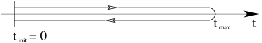
Figure 1: Closed real-time path $\mathcal{C}$. This time path was invented by Schwinger Schwinger:1960qe and applied to non-equilibrium problems by Keldysh Keldysh:1964ud . In order to avoid the doubling of the degrees of freedom, we use the form presented in Ref. Danielewicz:1982kk .

In the present work we extent our comparison of Boltzmann and Kadanoff-Baym equations to a chirally invariant Yukawa-type quantum field theory coupling fermions with scalars. We start from the 2PI effective action Jackiw:1974cv ; Cornwall:1974vz and derive the Kadanoff-Baym equations by requiring that the 2PI effective action be stationary with respect to variations of the complete connected two-point functions Calzetta:1986cq ; Berges:2002wr . First, this guarantees that the Kadanoff-Baym equations conserve the average energy density as well as global charges baym1961a ; Baym:1962sx ; Ivanov:1998nv , and second, the 2PI effective action has proven to be an efficient and reliable tool for the description of quantum fields out of thermal equilibrium in numerous previous treatments Berges:2000ur ; Berges:2001fi ; Berges:2002wr ; Aarts:2001yn ; Aarts:2003bk . In order to derive the corresponding Boltzmann equations, subsequently one has to employ a first-order gradient expansion, a Wigner transformation, the Kadanoff-Baym ansatz and the quasi-particle approximation baymKadanoff1962a ; Danielewicz:1982kk ; Ivanov:1999tj ; Knoll:2001jx ; Blaizot:2001nr . While Boltzmann equations describe the time evolution of particle number distributions, Kadanoff-Baym equations describe the evolution of the complete quantum mechanical two-point functions of the system. However, one can define effective particle number distributions, which can be obtained from the complete propagators and their time derivatives evaluated at equal times Berges:2001fi ; Berges:2002wr . Finally, we solve the Boltzmann and the Kadanoff-Baym equations numerically for highly symmetric systems in 3+1 space-time dimensions and compare their predictions on the evolution of these systems for various initial conditions.

II 2PI Effective Action

We consider a globally $SU(2)_{L}\times SU(2)_{R}\times U(1)_{B-L}$ symmetric quantum field theory with one generation of chiral leptons and a Higgs bidoublet with Dirac-Yukawa interactions Deshpande:1990ip . The Dirac fields are denoted with $\Psi_{l}^{\alpha}\left(x\right)$, where $\alpha$ is a Dirac index and $l\in\left\{\nu,e\right\}$ denotes the type of the leptons. Using the Pauli matrices, the (complex) Higgs bidoublet can be parameterized by real scalar fields denoted with $\Phi_{a}\left(x\right)$, where $a\in\left\{0,\ldots,3\right\}$. In this notation the Lagrangian density takes the form

$$\mathscr{L} = -{\bar{\Psi}}\not{\hbox{\kern-2.0pt$\partial$}}\Psi-\frac{1}{2}\Big{(}\partial_{\mu}\Phi_{a}\Big{)}\Big{(}\partial^{\mu}\Phi_{a}\Big{)}-\frac{1}{2}m_{B}^{2}\Phi_{a}\Phi_{a}$$

$${}-\lambda\left(\Phi_{a}\Phi_{a}\right)^{2}-i\eta{\bar{\Psi}}\Phi_{a}\left(\sigma_{a}P_{R}-{\sigma}^{\dagger}_{a}P_{L}\right)\Psi\;.$$

Although we refer to the scalar fields as Higgs fields, we would like to note that this theory is equivalent to the linear $\sigma$-model Schwinger:1957em ; polkinghorne1958a ; Gell-Mann:1960np , which can be used to describe low-energy quark-meson dynamics in two-flavor QCD. This and a similar model have been considered in a related context in Refs. Berges:2002wr ; Berges:2004ce .

Since we will compute the evolution of the two-point Green’s functions for non-equilibrium initial conditions, already the classical action has to be defined on the closed Schwinger-Keldysh real-time contour, shown in Figure 1. The free inverse propagators can then be read off the free part of the classical action:

$$I_{0} = -\int\limits_{\mathcal{C}}d^{4}x\;d^{4}y\Bigg{[}{\bar{\Psi}}_{l}\left(x\right)S_{0,lm}^{-1}\left(x,y\right)\Psi_{m}\left(y\right)$$

$${}+\frac{1}{2}\Phi_{a}\left(x\right)G_{0,ab}^{-1}\left(x,y\right)\Phi_{b}\left(y\right)\Bigg{]}\;,$$

where the inverse free propagators are given by

$$G_{0,ab}^{-1}\left(x,y\right)=\left(\partial_{x^{\mu}}\partial_{y_{\mu}}+m_{B}^{2}\right)\delta_{\mathcal{C}}\left(x-y\right)\delta_{ab}$$ (1)

and

$$S_{0,lm}^{-1}\left(x,y\right)=\not{\hbox{\kern-2.0pt$\partial$}}_{x}\delta_{\mathcal{C}}\left(x-y\right)\delta_{lm}\;.$$ (2)

We consider a system without symmetry breaking, i. e. $\left\langle\Phi_{a}\left(x\right)\right\rangle=0$. In this case the full connected Schwinger-Keldysh propagators are given by

$$G_{ab}\left(x,y\right)=\left\langle T_{\mathcal{C}}\left\{\Phi_{a}\left(x\right)\Phi_{b}\left(y\right)\right\}\right\rangle$$ (3)

and

$$S_{lm}^{\alpha\beta}\left(x,y\right)=\left\langle T_{\mathcal{C}}\left\{\Psi_{l}^{\alpha}\left(x\right){\bar{\Psi}}_{m}^{\beta}\left(y\right)\right\}\right\rangle\;,$$ (4)

so that the 2PI effective action can be written in the form

$$\Gamma\left[G,S\right] = \frac{i}{2}\mbox{tr}_{\mathcal{C}}\log_{\mathcal{C}}\left[G^{-1}\right]-\frac{1}{2}\mbox{tr}_{\mathcal{C}}\left[G_{0}^{-1}G\right]$$ (5)

$${}-i\mbox{tr}_{\mathcal{C}}\log_{\mathcal{C}}\left[S^{-1}\right]+\mbox{tr}_{\mathcal{C}}\left[S_{0}^{-1}S\right]$$

$${}+\Gamma_{2}\left[G,S\right]+const\;.$$

The square brackets indicate that the trace, the logarithm and the product of the propagators have to be taken in the functional sense, and the subscript $\mathcal{C}$ reminds us that integrals over time are running along the closed real-time contour. $i\Gamma_{2}\left[G,S\right]$ is the sum of all two-particle irreducible vacuum diagrams, where internal lines represent the complete connected propagators $S$ and $G$. In this work we apply the loop expansion of the 2PI effective action up to two-loop order. The diagrams contributing to $\Gamma_{2}$ in this approximation are shown in Figure 2. Using the abbreviation

Figure 2: Two-loop contribution to $\Gamma_{2}\left[G,S\right]$. Full (dashed) lines represent the complete connected lepton (Higgs) propagator $S$ ($G$).

$$H_{a,lm}^{\alpha\beta}=i\eta\left[\left(\sigma_{a}\right)_{lm}P_{R}^{\alpha\beta}-\left({\sigma}^{\dagger}_{a}\right)_{lm}P_{L}^{\alpha\beta}\right]$$

we find

$$\Gamma_{2}\left[G,S\right]=-\lambda\int\limits_{\mathcal{C}}d^{4}x\Big{[}G_{aa}\left(x,x\right)G_{bb}\left(x,x\right)$$

$${}+2G_{ab}\left(x,x\right)G_{ab}\left(x,x\right)\Big{]}$$

$${}-\frac{i}{2}\int\limits_{\mathcal{C}}d^{4}x\;d^{4}y\;G_{ab}\left(x,y\right)\mbox{tr}\Big{(}H_{a}S\left(x,y\right)H_{b}S\left(y,x\right)\Big{)}\;,$$

where the trace runs over Dirac and lepton type indices.

III Kadanoff-Baym Equations

Figure 3: One-loop contribution to the Higgs self-energy.

Figure 4: One-loop contribution to the lepton self-energy.

The equations of motion for the complete propagators read

$$\frac{\delta\Gamma\left[G,S\right]}{\delta G_{ba}\left(y,x\right)}=0\quad\mbox{and}\quad\frac{\delta\Gamma\left[G,S\right]}{\delta S_{ml}^{\beta\alpha}\left(y,x\right)}=0\;.$$ (6)

They are equivalent to the corresponding self-consistent Schwinger-Dyson equations

$$G^{-1}_{ab}\left(x,y\right)=iG^{-1}_{0,ab}\left(x,y\right)-\Pi_{ab}\left(x,y\right)$$ (7)

and

$$S^{-1}_{lm}\left(x,y\right)=iS^{-1}_{0,lm}\left(x,y\right)-\Sigma_{lm}\left(x,y\right)\;,$$ (8)

where the proper self-energies are given by

$$\Pi_{ab}\left(x,y\right)=2i\frac{\delta\Gamma_{2}\left[G,S\right]}{\delta G_{ba}\left(y,x\right)}$$ (9)

$$= -4\lambda i\delta_{\mathcal{C}}\left(x-y\right)\Big{(}G_{dd}\left(x,x\right)\delta_{ab}+2G_{ab}\left(x,x\right)\Big{)}$$

$${}+\mbox{tr}\Big{(}H_{a}S\left(x,y\right)H_{b}S\left(y,x\right)\Big{)}$$

and

$$\Sigma_{lm}^{\alpha\beta}\left(x,y\right)=-i\frac{\delta\Gamma_{2}\left[G,S\right]}{\delta S_{ml}^{\beta\alpha}\left(y,x\right)}$$ (10)

$$= -H_{a,lk}^{\alpha\gamma}H_{b,nm}^{\delta\beta}S_{kn}^{\gamma\delta}\left(x,y\right)G_{ab}\left(x,y\right)\;.$$

Next, we define the spectral function

$$G_{\varrho,ab}\left(x,y\right)=i\left\langle\left[\Phi_{a}\left(x\right),\Phi_{b}\left(y\right)\right]_{-}\right\rangle$$

and the statistical propagator

$$G_{F,ab}\left(x,y\right)=\frac{1}{2}\left\langle\left[\Phi_{a}\left(x\right),\Phi_{b}\left(y\right)\right]_{+}\right\rangle$$

for the Higgs bosons, so that we can write the complete Higgs propagator as

$$G\left(x,y\right)=G_{F}\left(x,y\right)-\frac{i}{2}\mbox{sign}_{\mathcal{C}}\left(x^{0}-y^{0}\right)G_{\varrho}\left(x,y\right)\;.$$ (11)

In the case of real scalar fields the spectral function and the statistical propagator are real-valued quantities Berges:2001fi . In a similar way, we also define the spectral function

$$S_{\varrho,lm}^{\alpha\beta}\left(x,y\right)=i\left\langle\left[\Psi_{l}^{\alpha}\left(x\right),{\bar{\Psi}}_{m}^{\beta}\left(y\right)\right]_{+}\right\rangle$$ (12)

and the statistical propagator

$$S_{F,lm}^{\alpha\beta}\left(x,y\right)=\frac{1}{2}\left\langle\left[\Psi_{l}^{\alpha}\left(x\right),{\bar{\Psi}}_{m}^{\beta}\left(y\right)\right]_{-}\right\rangle$$ (13)

for the leptons, so that we can decompose the complete lepton propagator according to

$$S\left(x,y\right)=S_{F}\left(x,y\right)-\frac{i}{2}\mbox{sign}_{\mathcal{C}}\left(x^{0}-y^{0}\right)S_{\varrho}\left(x,y\right)\;.$$ (14)

Then, using Eqs. (11) and (14), we can decompose the Higgs self-energy (9) as well as the lepton self-energy (10) according to:

$$\Pi\left(x,y\right) = -i\delta_{\mathcal{C}}\left(x-y\right)\Pi^{(local)}\left(x\right)$$

$${}+\Pi_{F}\left(x,y\right)-\frac{i}{2}\mbox{sign}_{\mathcal{C}}\left(x^{0}-y^{0}\right)\Pi_{\varrho}\left(x,y\right)$$

and

$$\Sigma\left(x,y\right)=\Sigma_{F}\left(x,y\right)-\frac{i}{2}\mbox{sign}_{\mathcal{C}}\left(x^{0}-y^{0}\right)\Sigma_{\varrho}\left(x,y\right)\;.$$

The local part of the Higgs self-energy causes a mass shift only, wherefore we define the effective mass by

$$M_{ab}^{2}\left(x\right)=m_{B}^{2}\delta_{ab}+\Pi_{ab}^{(local)}\left(x\right)$$

$$= m_{B}^{2}\delta_{ab}+4\lambda\Big{(}G_{dd}\left(x,x\right)\delta_{ab}+2G_{ab}\left(x,x\right)\Big{)}\;.$$

After convoluting Eqs. (7) and (8) from the right with the corresponding complete propagators, we observe that both equations split into two complementary evolution equations for the statistical propagators and the spectral functions, respectively Berges:2002wr :

$$\left(-\partial_{x^{\mu}}\partial_{x_{\mu}}\delta_{ac}+M_{ac}^{2}\left(x\right)\right)G_{F,cb}\left(x,y\right)$$ (16)

$$= \int\limits_{0}^{y^{0}}d^{4}z\;\Pi_{F,ac}\left(x,z\right)G_{\varrho,cb}\left(z,y\right)$$

$${}-\int\limits_{0}^{x^{0}}d^{4}z\;\Pi_{\varrho,ac}\left(x,z\right)G_{F,cb}\left(z,y\right)\;,$$

$$\left(-\partial_{x^{\mu}}\partial_{x_{\mu}}\delta_{ac}+M_{ac}^{2}\left(x\right)\right)G_{\varrho,cb}\left(x,y\right)$$ (17)

$$= -\int\limits_{y^{0}}^{x^{0}}d^{4}z\;\Pi_{\varrho,ac}\left(x,z\right)G_{\varrho,cb}\left(z,y\right)\;,$$

$$\not{\hbox{\kern-2.0pt$\partial$}}_{x}S_{F,lm}\left(x,y\right)=\int\limits_{0}^{y^{0}}d^{4}z\;\Sigma_{F,lk}\left(x,z\right)S_{\varrho,km}\left(z,y\right)$$ (18)

$${}-\int\limits_{0}^{x^{0}}d^{4}z\;\Sigma_{\varrho,lk}\left(x,z\right)S_{F,km}\left(z,y\right)\hskip 42.67912pt$$

and

$$\not{\hbox{\kern-2.0pt$\partial$}}_{x}S_{\varrho,lm}\left(x,y\right)=-\int\limits_{y^{0}}^{x^{0}}d^{4}z\;\Sigma_{\varrho,lk}\left(x,z\right)S_{\varrho,km}\left(z,y\right)\;.$$ (19)

Nowadays, it is practically impossible to solve the Kadanoff-Baym equations numerically in this general form. However, for initial conditions which are invariant under spatial translations, spatial rotations, parity, charge conjugation, and chiral transformations, the propagators take the form Berges:2002wr

$$G_{ab}\left(x,y\right)=\int\frac{d^{3}k}{\left(2\pi\right)^{3}}\;\exp\Big{(}i\bm{k}\left(\bm{x}-\bm{y}\right)\Big{)}G\left(x^{0},y^{0},k\right)\delta_{ab}$$ (20)

and

$$S_{lm}\left(x,y\right)=\int\frac{d^{3}k}{\left(2\pi\right)^{3}}\;\exp\Big{(}i\bm{k}\left(\bm{x}-\bm{y}\right)\Big{)}$$

$${}\times\left(S_{V}^{0}\left(x^{0},y^{0},k\right)\gamma_{0}-i\frac{k^{j}}{k}S_{V}\left(x^{0},y^{0},k\right)\gamma_{j}\right)\;\delta_{lm}\;,$$

where $k=\left|\bm{k}\right|$. The index $V$ indicates that $S_{V}^{\mu}$ would transform as a vector under a Lorentz transformation. Due to CP invariance, the statistical and spectral vector components of the lepton propagator satisfy

$$\begin{array}[]{rcrcr}S_{V,F}^{0}\left(x^{0},y^{0},k\right)\!&=&\!-S_{V,F}^{0}\left(y^{0},x^{0},k\right)\!&=&\!S_{V,F}^{0^{\scriptstyle\ast}}\left(x^{0},y^{0},k\right)\\[5.69054pt] S_{V,F}\left(x^{0},y^{0},k\right)\!&=&\!S_{V,F}\left(y^{0},x^{0},k\right)\!&=&\!S_{V,F}^{\ast}\left(x^{0},y^{0},k\right)\\[5.69054pt] S_{V,\varrho}^{0}\left(x^{0},y^{0},k\right)\!&=&\!S_{V,\varrho}^{0}\left(y^{0},x^{0},k\right)\!&=&\!S_{V,\varrho}^{0^{\scriptstyle\ast}}\left(x^{0},y^{0},k\right)\\[5.69054pt] S_{V,\varrho}\left(x^{0},y^{0},k\right)\!&=&\!-S_{V,\varrho}\left(y^{0},x^{0},k\right)\!&=&\!S_{V,\varrho}^{\ast}\left(x^{0},y^{0},k\right)\end{array}$$ (22)

Thus, the explicit factor of $i$ makes $S_{V,F}^{0}$, $S_{V,F}$, $S_{V,\varrho}^{0}$ and $S_{V,\varrho}$ real-valued quantities:

$$\mbox{Im}\left(S_{V,F}^{0}\right)=\mbox{Im}\left(S_{V,F}\right)=\mbox{Im}\left(S_{V,\varrho}^{0}\right)=\mbox{Im}\left(S_{V,\varrho}\right)=0\;.$$ (23)

Furthermore, the canonical equal-time anti-commutation relations for fermion fields imply

$$S_{V,\varrho}^{0}\left(t,t,k\right)=1\qquad\mbox{and}\qquad S_{V,\varrho}\left(t,t,k\right)=0\;,$$ (24)

the second equality being consistent with the anti-symmetry of the space-like vector-component of the lepton spectral function, cf. Eq. (22). Of course, the relations (20), (III), (22) and (23) also hold for the corresponding self energies, so that the Kadanoff-Baym equations can be simplified drastically. The simplified Kadanoff-Baym equations for the Higgs propagator read Berges:2002wr

$$\left[\partial^{2}_{x^{0}}+k^{2}+M^{2}\left(x^{0}\right)\right]G_{F}\left(x^{0},y^{0},k\right)$$ (25)

$$= \int\limits_{0}^{y^{0}}dz^{0}\;\Pi_{F}\left(x^{0},z^{0},k\right)G_{\varrho}\left(z^{0},y^{0},k\right)-\int\limits_{0}^{x^{0}}dz^{0}\;\Pi_{\varrho}\left(x^{0},z^{0},k\right)G_{F}\left(z^{0},y^{0},k\right)$$

and

$$\left[\partial^{2}_{x^{0}}+k^{2}+M^{2}\left(x^{0}\right)\right]G_{\varrho}\left(x^{0},y^{0},k\right)=-\int\limits_{y^{0}}^{x^{0}}dz^{0}\;\Pi_{\varrho}\left(x^{0},z^{0},k\right)G_{\varrho}\left(z^{0},y^{0},k\right)\;.$$ (26)

In the same way, the 128 complex-valued Kadanoff-Baym equations (18) and (19) for the lepton propagator can be reduced to the following 4 real-valued equations Berges:2002wr :

$$\partial_{x^{0}}S_{V,F}^{0}\left(x^{0},y^{0},k\right)+kS_{V,F}\left(x^{0},y^{0},k\right)$$

$$= {}-\int\limits_{0}^{y^{0}}dz^{0}\;\Big{[}\Sigma_{V,F}^{0}\left(x^{0},z^{0},k\right)S_{V,\varrho}^{0}\left(z^{0},y^{0},k\right)+\Sigma_{V,F}\left(x^{0},z^{0},k\right)S_{V,\varrho}\left(z^{0},y^{0},k\right)\Big{]}$$

$${}+\int\limits_{0}^{x^{0}}dz^{0}\;\Big{[}\Sigma_{V,\varrho}^{0}\left(x^{0},z^{0},k\right)S_{V,F}^{0}\left(z^{0},y^{0},k\right)+\Sigma_{V,\varrho}\left(x^{0},z^{0},k\right)S_{V,F}\left(z^{0},y^{0},k\right)\Big{]}\;,$$

$$\partial_{x^{0}}S_{V,F}\left(x^{0},y^{0},k\right)-kS_{V,F}^{0}\left(x^{0},y^{0},k\right)$$

$$= \int\limits_{0}^{y^{0}}dz^{0}\;\Big{[}\Sigma_{V,F}\left(x^{0},z^{0},k\right)S_{V,\varrho}^{0}\left(z^{0},y^{0},k\right)-\Sigma_{V,F}^{0}\left(x^{0},z^{0},k\right)S_{V,\varrho}\left(z^{0},y^{0},k\right)\Big{]}$$

$${}-\int\limits_{0}^{x^{0}}dz^{0}\;\Big{[}\Sigma_{V,\varrho}\left(x^{0},z^{0},k\right)S_{V,F}^{0}\left(z^{0},y^{0},k\right)-\Sigma_{V,\varrho}^{0}\left(x^{0},z^{0},k\right)S_{V,F}\left(z^{0},y^{0},k\right)\Big{]}\;,$$

$$\partial_{x^{0}}S_{V,\varrho}^{0}\left(x^{0},y^{0},k\right)+kS_{V,\varrho}\left(x^{0},y^{0},k\right)$$

$$= \int\limits_{y^{0}}^{x^{0}}dz^{0}\;\Big{[}\Sigma_{V,\varrho}^{0}\left(x^{0},z^{0},k\right)S_{V,\varrho}^{0}\left(z^{0},y^{0},k\right)+\Sigma_{V,\varrho}\left(x^{0},z^{0},k\right)S_{V,\varrho}\left(z^{0},y^{0},k\right)\Big{]}$$

and

$$\partial_{x^{0}}S_{V,\varrho}\left(x^{0},y^{0},k\right)-kS_{V,\varrho}^{0}\left(x^{0},y^{0},k\right)$$

$$= -\int\limits_{y^{0}}^{x^{0}}dz^{0}\;\Big{[}\Sigma_{V,\varrho}\left(x^{0},z^{0},k\right)S_{V,\varrho}^{0}\left(z^{0},y^{0},k\right)-\Sigma_{V,\varrho}^{0}\left(x^{0},z^{0},k\right)S_{V,\varrho}\left(z^{0},y^{0},k\right)\Big{]}\;.$$

The expressions for the Higgs and lepton self-energies are given in App. A. As explained in more detail in Ref. Berges:2002wr , one can define an effective kinetic energy distribution $\omega\left(t,k\right)$, as well as effective scalar and fermion particle number distributions $n_{s}\left(t,k\right)$ and $n_{f}\left(t,k\right)$, which can be obtained from the statistical propagators according to

$$\omega^{2}\left(t,k\right)=\left(\frac{\partial_{x^{0}}\partial_{y^{0}}G_{F}\left(x^{0},y^{0},k\right)}{G_{F}\left(x^{0},y^{0},k\right)}\right)_{x^{0}=y^{0}=t}\;,$$ (31)

$$n_{s}\left(t,k\right)=\omega\left(t,k\right)G_{F}\left(t,t,k\right)-\frac{1}{2}\;.$$ (32)

and

$$n_{f}\left(t,k\right)=\frac{1}{2}-S_{V,F}\left(t,t,k\right)\;.$$ (33)

The definition of such particle numbers is necessary in order to make contact to Boltzmann equations, e. g. when comparing numerical solutions of Boltzmann and Kadanoff-Baym equations, which we will do in Sect. V. We emphasize, however, that the Kadanoff-Baym equations are self-consistent evolution equations for the complete propagators of our system, and that one has to follow the evolution of the two-point functions throughout the complete $x^{0}$-$y^{0}$-plane (of course, constrained to the part with $x^{0}\geq 0$ and $y^{0}\geq 0$). One can then follow the evolution of the effective particle number densities along the bisecting line of this plane.

IV Boltzmann Equations

In this section we briefly sketch the standard way of deriving Boltzmann equations from Kadanoff-Baym equations baymKadanoff1962a ; Danielewicz:1982kk ; Blaizot:2001nr ; Berges:2004pu ; Prokopec:2003pj ; Prokopec:2004ic . One has to employ a Wigner transformation, a first-order gradient expansion, the Kadanoff-Baym ansatz and the quasi-particle approximation.

First, we subtract Eq. (25) (Eq. (III)) with $x^{0}$ and $y^{0}$ interchanged from Eq. (25) (Eq. (III)). Then we re-parameterize the propagators and the self energies by center and relative times, e. g.

$$G\left(u^{0},v^{0},k\right)=G\left(\frac{u^{0}+v^{0}}{2},u^{0}-v^{0},k\right)\;.$$

Next, we define the center time $t=\frac{x^{0}+y^{0}}{2}$ and the relative time $s^{0}=x^{0}-y^{0}$, and observe on the left hand side of the difference equations that

$$\partial_{x^{0}}\partial_{x^{0}}-\partial_{y^{0}}\partial_{y^{0}}=2\partial_{t}\partial_{s^{0}}$$

and

$$\partial_{x^{0}}+\partial_{y^{0}}=\partial_{t}$$

are automatically of first order in $\partial_{t}$. Furthermore, we Taylor expand the effective masses on the left hand side of the difference equation for the scalars as well as the propagators and self energies on the right hand sides of both difference equations to first order in $\partial_{t}$ around $t$. After that, we Fourier transform the difference equations with respect to the relative time $s^{0}$. The Wigner transformed scalar statistical propagator and scalar spectral function are given by

$$G_{F}\left(t,\omega,k\right) = \int ds^{0}\;\exp\left(i\omega s^{0}\right)G_{F}\left(t,s^{0},k\right)\;,$$

$$G_{\varrho}\left(t,\omega,k\right) = -i\int ds^{0}\;\exp\left(i\omega s^{0}\right)G_{\varrho}\left(t,s^{0},k\right)\;.$$

As $G_{\varrho}\left(t,s^{0},k\right)$ is a real-valued odd function of the relative time $s^{0}$, we introduced an explicit factor of $-i$ in order to make its Wigner transform again a real-valued function. For similar reasons we also introduce a factor of $-i$ for the Wigner transforms of $S_{V,\varrho}\left(t,s^{0},k\right)$, $S_{V,F}^{0}\left(t,s^{0},k\right)$, $S_{V,R}^{0}\left(t,s^{0},k\right)$, and $S_{V,A}^{0}\left(t,s^{0},k\right)$, as well as the corresponding self energies. In order to be able to really perform the Fourier transformation, we have to send the initial time to $-\infty$. At least for large $x^{0}$ and $y^{0}$ this can be justified by taking into account that correlations between earlier and later times are suppressed exponentially Berges:2001fi ; Lindner:2005kv . For early times, however, this is certainly not the case. The result of all these transformations are quantum-kinetic equations for the statistical propagators $G_{F}$ and $S_{V,F}^{0}$ Ivanov:1999tj ; Knoll:2001jx ; Blaizot:2001nr ; Berges:2002wt ; Juchem:2004cs ; Berges:2005vj ; Berges:2005md :

$$-\left\{\Omega;\;G_{F}\right\}_{PB}=\Pi_{\varrho}G_{F}-\Pi_{F}G_{\varrho}+\left\{\Pi_{F};\;\mbox{Re}\left(G_{R}\right)\right\}_{PB}$$ (34)

and

$$\left\{W;\;S_{V,F}^{0}\right\}_{PB}=\Sigma_{V,\varrho}^{0}S_{V,F}^{0}-\Sigma_{V,F}^{0}S_{V,\varrho}^{0}+\Sigma_{V,\varrho}S_{V,F}$$

$${}-\Sigma_{V,F}S_{V,\varrho}-\left\{\Sigma_{V,F}^{0};\;\mbox{Re}\left(S_{V,R}^{0}\right)\right\}_{PB}$$

$${}+\left\{\mbox{Re}\left(\Sigma_{V,R}\right);\;S_{V,F}\right\}_{PB}+\left\{\Sigma_{V,F};\;\mbox{Re}\left(S_{V,R}\right)\right\}_{PB}\;,$$

where the Poisson brackets are defined by

$$\left\{f;\;g\right\}_{PB}=-\Big{[}\partial_{t}f\Big{]}\Big{[}\partial_{\omega}g\Big{]}+\Big{[}\partial_{\omega}f\Big{]}\Big{[}\partial_{t}g\Big{]}\;.$$

The auxiliary functions

$$\Omega\left(t,\omega,k\right)=-\omega^{2}+k^{2}+M^{2}\left(t\right)+\mbox{Re}\left(\Pi_{R}\left(t,\omega,k\right)\right)$$

and

$$W\left(t,\omega,k\right)=\omega+\mbox{Re}\left(\Sigma_{V,R}^{0}\left(t,\omega,k\right)\right)$$

have been introduced to simplify the notation. Employing the first-order Taylor expansion is clearly not justifiable for early times when the equal-time propagator is rapidly oscillating Berges:2000ur ; Lindner:2005kv . Consequently, one might expect that the above quantum-kinetic equations and also the Boltzmann equations, which we derive subsequently, fail to describe the early-time evolution and that errors accumulated for early times cannot be remedied at late times. In fact, the first-order gradient expansion is motivated by equilibrium considerations: In equilibrium the propagator depends on the relative coordinates only. There is no dependence on the center coordinates, and one may hope that there are situations where the propagator depends only moderately on the center coordinates. This is clearly the case for late times when our system is sufficiently close to equilibrium. However, already after moderate times the rapid oscillations mentioned above, have died out and are followed by a monotonous drifting regime Berges:2001fi ; Lindner:2005kv . In this drifting regime the second derivative with respect to $t$ should be negligible as compared to the first-order derivative, and a consistent Taylor expansion can be justified even though the system may still be far from equilibrium. Here, it is crucial that the Taylor expansion is performed consistently for two reasons: First, this guarantees that the quantum-kinetic equations satisfy exactly the same conservation laws as the full Kadanoff-Baym equations do Knoll:2001jx . Second, it has been shown that neglecting the Poisson brackets severely restricts the range of validity of the quantum-kinetic transport equations Berges:2005ai ; Berges:2005md .

In order to derive Boltzmann equations from the quantum-kinetic equations for the statistical propagators (34) and (IV), first we have to discard the Poisson brackets on the right-hand sides, thereby sacrificing the consistency of the gradient expansion. On the left-hand sides we remove the time dependence of the auxiliary quantities $\Omega$ and $W$. We take

$$W\left(t,\omega,k\right)=\omega$$

and

$$\Omega\left(t,\omega,k\right)=-\omega^{2}+k^{2}+m^{2}\;,$$

where $m$ is the thermal mass of the scalars. After that, we employ the Kadanoff-Baym ansatz

$$G_{F}\left(t,\omega,k\right)=G_{\varrho}\left(\omega,k\right)\left(\frac{1}{2}+n_{s}\left(t,\omega,k\right)\right)$$ (36)

and

$$S_{F}\left(t,\omega,k\right)=S_{\varrho}\left(\omega,k\right)\left(\frac{1}{2}-n_{f}\left(t,\omega,k\right)\right)$$ (37)

which also can be motivated by equilibrium considerations. In fact, this is a generalization of the fluctuation-dissipation theorem, which states that, for a system in thermal equilibrium, the statistical propagator is proportional to the spectral function. The fluctuation dissipation theorem can be recovered from Eqs. (36) and (37) by discarding the dependence on the center time $t$ and fixing $n_{s}$ and $n_{f}$ to be the Bose-Einstein and Fermi-Dirac distribution function, respectively. The last approximation, which is necessary to arrive at the Boltzmann equations, is the so-called quasi-particle (or on-shell) approximation. For the scalars this means that the spectral function takes the form

$$G_{\varrho}\left(\omega,k\right)=\frac{\pi}{E\left(k\right)}\Big{(}\delta\left(\omega-E\left(k\right)\right)-\delta\left(\omega+E\left(k\right)\right)\Big{)}\;,$$

where the quasi-particle energy is given by

$$E\left(k\right)=\sqrt{m^{2}+k^{2}}\;.$$

For the lepton spectral function we assume

$$S_{V,\varrho}^{0}\left(\omega,k\right) = \pi\left(\delta\left(\omega-k\right)+\delta\left(\omega+k\right)\right)\;,$$

$$S_{V,\varrho}\left(\omega,k\right) = \pi\left(\delta\left(\omega-k\right)-\delta\left(\omega+k\right)\right)\;.$$

Once more, we would like to stress that the exact time evolution of the spectral functions is determined by the Kadanoff-Baym equations. It has been shown that the spectral function can be parameterized by a Breit-Wigner function with a non-vanishing width Aarts:2001qa ; Juchem:2003bi . To reduce the width of this Breit-Wigner curve to zero is certainly not a controllable approximation and leads to very large qualitative discrepancies between the results produced by Kadanoff-Baym and Boltzmann equations. In fact this approximation can only be justified if our system consists of stable, or at least very long-lived, quasi-particles, whose mass is much larger than their decay width. We also would like to note that a completely self-consistent determination of the thermal mass in the framework of the Boltzmann equation requires the solution of an integral equation for $E\left(k\right)$, which would drastically increase the complexity of our numerics. As none of our physical results depend on the exact value of the thermal mass, for convenience, we use the equilibrium value of the thermal scalar mass as determined by the Kadanoff-Baym equations. Eventually, we define the quasi-particle number densities by

$$n_{s}\left(t,k\right)=n_{s}\left(t,E\left(k\right),k\right)$$

and

$$n_{f}\left(t,k\right)=n_{f}\left(t,k,k\right)\;.$$

After equating the positive energy components in Eqs. (34) and (IV) we arrive at the following Boltzmann equations:

$$\partial_{t}n_{s}\left(t,k\right)=2\pi\eta^{2}\int\frac{d^{3}p}{\left(2\pi\right)^{3}}\int d^{3}q\;\delta^{3}\left(\bm{k}-\bm{p}-\bm{q}\right)$$ (38)

$${}\times\delta\left(E\left(k\right)-p-q\right)\frac{1}{E(k)}\left(1-\frac{\bm{p}\bm{q}}{pq}\right)$$

$${}\times\bigg{[}\Big{(}n_{s}\left(t,k\right)+1\Big{)}n_{f}\left(t,p\right)n_{f}\left(t,q\right)$$

$${}-n_{s}\left(t,k\right)\Big{(}n_{f}\left(t,p\right)-1\Big{)}\Big{(}n_{f}\left(t,q\right)-1\Big{)}\bigg{]}$$

and

$$\partial_{t}n_{f}\left(t,k\right)=2\pi\eta^{2}\int\frac{d^{3}p}{\left(2\pi\right)^{3}}\int d^{3}q\;\delta^{3}\left(\bm{k}+\bm{p}-\bm{q}\right)$$ (39)

$${}\times\delta\left(k+p-E\left(q\right)\right)\frac{1}{E(q)}\left(1-\frac{\bm{k}\bm{p}}{kp}\right)$$

$${}\times\bigg{[}\Big{(}n_{f}\left(t,k\right)-1\Big{)}\Big{(}n_{f}\left(t,p\right)-1\Big{)}n_{s}\left(t,q\right)$$

$${}-n_{f}\left(t,k\right)n_{f}\left(t,p\right)\Big{(}n_{s}\left(t,q\right)+1\Big{)}\bigg{]}\;.$$

Exploiting isotropy the above 6-dimensional Boltzmann collision integrals can be reduced to 1-dimensional integrals:

$$\partial_{t}n_{s}\left(t,k\right)=\frac{2\eta^{2}}{\pi^{2}E\left(k\right)}\int\limits_{0}^{\infty}dp\;\theta\left(q_{0}\right)J_{s}\left(k,p,q_{0}\right)$$

$${}\times\bigg{[}\Big{(}n_{s}\left(t,k\right)+1\Big{)}n_{f}\left(t,p\right)n_{f}\left(t,q_{0}\right)$$

$${}-n_{s}\left(t,k\right)\Big{(}n_{f}\left(t,p\right)-1\Big{)}\Big{(}n_{f}\left(t,q_{0}\right)-1\Big{)}\bigg{]}\;,$$

$$\partial_{t}n_{f}\left(t,k\right)=\frac{2\eta^{2}}{\pi^{2}}\int\limits_{0}^{\infty}dq\;\theta\left(p_{0}\right)\;\frac{q}{E\left(q\right)}J_{f}\left(k,p_{0},q\right)$$ (41)

$${}\times\bigg{[}\Big{(}n_{f}\left(t,k\right)-1\Big{)}\Big{(}n_{f}\left(t,p_{0}\right)-1\Big{)}n_{s}\left(t,q\right)$$

$${}-n_{f}\left(t,k\right)n_{f}\left(t,p_{0}\right)\Big{(}n_{s}\left(t,q\right)+1\Big{)}\bigg{]}\;.$$

The details of these calculations and the definitions of all of the auxiliary quantities are given in App. C. This simplification of the collision integrals is crucial in order to implement efficient computer programs for the numerical solution of the Boltzmann equations.

In this section we showed that the derivation of Boltzmann equations from Kadanoff-Baym equations requires a number of non-trivial approximations and assumptions. One has to employ a first-order gradient expansion, a Wigner transformation and a quasi-particle approximation. In this sense, one can consider the Kadanoff-Baym equations as quantum Boltzmann equations re-summing the gradient expansion up to infinite order and including memory and off-shell effects.

V Comparing Boltzmann vs. Kadanoff-Baym 

V.1 Initial Conditions and Numerical Settings

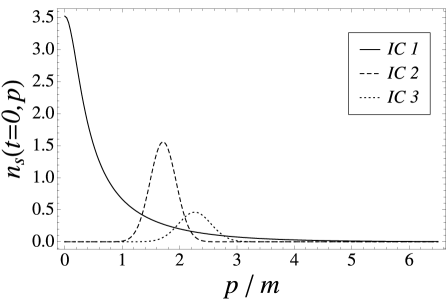
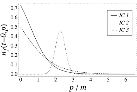
Figure 5: Initial particle number distributions for scalars (left) and fermions (right). These distributions define the initial conditions (IC) for which we numerically solved the Boltzmann and Kadanoff-Baym equations. All initial conditions correspond to the same (conserved) average energy density. Above that, for the initial conditions IC1 and IC2 also the sum of the initial average number densities agree.

In order to solve the Kadanoff-Baym equations numerically, we follow exactly the lines of Refs. Berges:2002wr ; Lindner:2005kv ; montvayMunster1994a on a lattice with $2000^{2}\times 32^{3}$ lattice sites. The values for the coupling constants are $\eta=1$ and $\lambda=0.25$. The initial conditions for the statistical propagators are determined by scalar and fermionic particle number distributions $n_{s}\left(t=0,p\right)$ and $n_{f}\left(t=0,p\right)$ according to

$$G_{F}\left(x^{0},y^{0},p\right)_{x^{0}=y^{0}=0} = \frac{n_{s}\left(t=0,p\right)+\frac{1}{2}}{\omega_{0}\left(p\right)}\;,$$

$$\left[\partial_{x^{0}}G_{F}\left(x^{0},y^{0},p\right)\right]_{x^{0}=y^{0}=0} = 0\;,$$

$$\left[\partial_{x^{0}}\partial_{y^{0}}G_{F}\left(x^{0},y^{0},p\right)\right]_{x^{0}=y^{0}=0}$$

$$= \omega_{0}\left(p\right)\left(n_{s}\left(t=0,p\right)+\frac{1}{2}\right)\;,$$

$$S_{V,F}^{0}\left(x^{0},y^{0},p\right)_{x^{0}=y^{0}=0} = 0\;,$$

$$S_{V,F}\left(x^{0},y^{0},p\right)_{x^{0}=y^{0}=0} = \frac{1}{2}-n_{f}\left(t=0,p\right)\;,$$

where $\omega_{0}\left(p\right)$ is the initial scalar kinetic energy distribution. On the other hand, the initial conditions for the spectral functions are determined by equal-time (anti-) commutation relations. We solve the Boltzmann and Kadanoff-Baym equations for three different sets of initial particle number distributions, which are shown in Figure 5. All initial conditions correspond to the same (conserved) average energy density. Above that, for the initial conditions IC1 and IC2 also the sum of the initial scalar and fermionic average particle number densities agree. The numerical solution of the Boltzmann equations proceeds along the lines of Ref. Lindner:2005kv . The scale in our plots is set by the scalar thermal mass $m=\omega_{eq}\left(p=0\right)$, where $\omega_{eq}\left(p\right)$ is the effective kinetic energy distribution (31) for sufficiently late time $t$.

V.2 Universality

Figs. 6 and 7 exhibit that the Kadanoff-Baym equations respect full universality: Figure 6 shows the time evolution of the particle number distributions for a fixed momentum mode. The particle number distributions start from different initial values and go through very different early-time evolutions. Nevertheless, in the case of the Kadanoff-Baym equations they all approach the same universal late-time value. Figure 7 shows the particle number distributions for times when equilibrium has effectively been reached. In the case of Kadanoff-Baym equations, we observe that the equilibrium number distributions agree exactly independent of the initial conditions, which proves that we could have shown the plots of Figure 6 for any momentum mode. In particular, the straight lines in Figure 7 prove that the equilibrium number distributions take the form of Bose-Einstein or Fermi-Dirac distribution functions with a universal temperature $T=2.3m$ and universally vanishing chemical potentials.

In contrast to this, Boltzmann equations maintain only a restricted universality. Figs. 6 and 7 reveal that only the initial conditions IC1 and IC2 lead to the same late-time behavior, which deviates significantly from the one approached by the third initial condition IC3. Again, the straightness of the lines in Figure 7 proves that the equilibrium number distributions take the Form of Bose-Einstein or Fermi-Dirac distribution functions. However, the different slopes of the lines indicate that the temperature is not the same for all initial conditions, and the non-vanishing y-axis intercepts indicate that Boltzmann equations may predict different non-vanishing chemical potentials. Fitted values for these quantities are given in Table 1.

The reason for the observed restriction of universality can be extracted from Figure 8 where we plotted the time evolution of the average particle number densities per degree of freedom

$$N_{s}\left(t\right)=\int\frac{d^{3}p}{\left(2\pi\right)^{3}}\;n_{s}\left(t,p\right)$$ (42)

and

$$N_{f}\left(t\right)=\int\frac{d^{3}p}{\left(2\pi\right)^{3}}\;n_{f}\left(t,p\right)$$ (43)

and their sum. Provided $\Phi$-derivable approximations are employed, Kadanoff-Baym equations conserve the average energy density as well as global charges baym1961a ; Baym:1962sx ; Ivanov:1998nv . However, as we consider systems with vanishing net charge density neither of the above average particle number densities has to be conserved, nor their sum. Indeed, Kadanoff-Baym equations include off-shell particle creation and annihilation Lindner:2005kv ; Aarts:2001qa , so that all of the quantities plotted in Figure 8 may change as time goes on and approach a universal equilibrium value.

In contrast to this, due to the quasi-particle (or on-shell) approximation the Boltzmann equations (IV) and (41) only include decay and recombination processes of the form

$$\mbox{1 scalar}\longleftrightarrow\mbox{2 fermions}\;.$$ (44)

More precisely, one of four scalars may decay into or be recombined from one of two fermion pairs. As a consequence the sum of the average particle number densities (42) and (43) is strictly conserved, as can be seen in Figure 8. Of course, this artificial constant of motion severely restricts the evolution of the particle number distributions. As a result, the Boltzmann equations maintain only a restricted universality and, as will be discussed in the next subsection, fail to describe the process of quantum-chemical equilibration.

V.3 Chemical Equilibration

Figure 6: Time evolution of the particle number distributions for a fixed momentum mode $p$. We see that Kadanoff-Baym equations respect full universality, whereas Boltzmann equations maintain only a restricted universality.

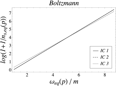
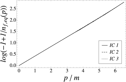
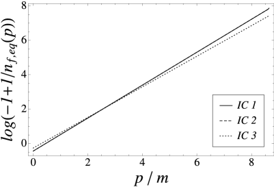
Figure 7: Equilibrium particle number distributions. The straight lines in these plots prove that in equilibrium the particle number distributions indeed take the form of Bose-Einstein or Fermi-Dirac distribution functions, where the temperature is given by the inverse slope and the chemical potential is proportional to the y-axis intercept. The Kadanoff-Baym equations lead to a universal temperature $T=2.3m$ and universally vanishing chemical potentials. The temperatures and chemical potentials predicted by the Boltzmann equations are given in Table 1.

$$\begin{array}[]{c|c|c|r|r|c}&T_{s}/m&T_{f}/m&\mu_{s}/m&\mu_{f}/m&\mu_{s}/\mu_{f}\\ \hline\cr IC1&1.044&1.044&0.910&0.455&1.999\\ IC2&1.044&1.044&0.910&0.455&2.001\\ IC3&1.125&1.124&0.586&0.293&1.997\end{array}$$

Table 1: Temperatures and chemical potentials as predicted by the Boltzmann equations. The values in this table have been obtained by fitting the equilibrium particle number distributions shown in Figure 7 against Bose-Einstein and Fermi-Dirac distribution functions, respectively.

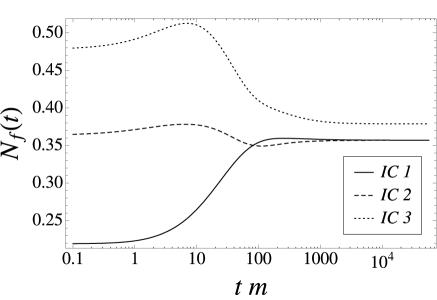
Figure 8: Time evolution of the average particle number densities and their sum. Kadanoff-Baym equations allow for a change of the latter quantity, whereas it is artificially conserved by Boltzmann equations. The quantitative disagreement of the average particle number densities can be attributed to different initial conditions and discretization schemes for the Boltzmann and the Kadanoff-Baym equations, and is of no relevance for the purpose of the present work.

In a system allowing for creation and annihilation of particles, the chemical potential of particles, whose total number is not restricted by any conserved quantity, must vanish in thermodynamic equilibrium. Accordingly, as we consider systems with vanishing net charge density the chemical potentials for scalars and fermions should vanish once equilibrium has been reached. Indeed, Kadanoff-Baym equations lead to universally vanishing chemical potentials. In contrast to this, as one can see in Table 1, the Boltzmann equations in general will give non-vanishing chemical potentials. For a system which includes only interactions of the form (44), in equilibrium the chemical potentials are expected to satisfy the relation

$$\mu_{s}=2\mu_{f}\;.$$

As one can see in the right-most column of Table 1, this relation is indeed fulfilled up to numerical errors $<0.3\%$. Thus, the Boltzmann equations (IV) and (41) lead to a classical chemical equilibrium. As mentioned above, however, quantum-chemical equilibrium requires that the chemical potentials vanish for systems with vanishing net charge density. In this sense, the non-vanishing chemical potentials in Table 1 indicate that the description of quantum-chemical equilibration is out of reach of the Boltzmann equations (IV) and (41).

V.4 Separation of Time Scales

As has been discussed in Ref. Lindner:2005kv in the framework of a purely scalar theory and in Ref. Berges:2004ce in the framework of the linear sigma model underlying our studies in this work, Kadanoff-Baym equations strongly separate the time scales between the kinetic and the complete thermodynamic (including chemical) equilibration. This phenomenon has been called prethermalization Berges:2004ce , and implies that certain quantities approach their equilibrium values on time scales which are dramatically shorter than the thermodynamic equilibration time.

As we have seen in this work and in Ref. Lindner:2005kv , standard Boltzmann equations cannot describe the phenomenon of quantum-chemical equilibration, and thus they also cannot describe the approach to the quantum-thermodynamic equilibrium. Consequently, standard Boltzmann equations cannot separate the time scales between the kinetic and the full thermodynamic equilibration and hence a description of prethermalization is out of reach of standard Boltzmann equations.

VI Conclusions

In this article we addressed the question how reliable Boltzmann equations are as approximations to Kadanoff-Baym equations in the framework of a chirally invariant Yukawa-type quantum field theory coupling scalars with fermions. Starting from the 2PI effective action, we reviewed the derivation of the Kadanoff-Baym equations and the approximations which are necessary to eventually arrive at standard Boltzmann equations. We solved the Boltzmann and Kadanoff-Baym equations numerically for highly symmetric systems in 3+1 space-time dimensions without any further approximations and compared their solutions for various non-equilibrium initial conditions.

We demonstrated that the Kadanoff-Baym equations respect universality: For systems with equal average energy density the late-time behavior coincides independent of the details of the initial conditions. In particular, independent of the initial conditions the particle number distributions, temperatures, chemical potentials and thermal masses predicted for times, when equilibrium has effectively been reached, coincide. Above that, Kadanoff-Baym equations incorporate the process of quantum-chemical equilibration: For systems with vanishing net charge density the chemical potentials vanish once equilibrium has effectively been reached. Last but not least, Kadanoff-Baym equations feature the phenomenon of prethermalization and separate the time scales between kinetic and full thermodynamic (including quantum-chemical) equilibration.

The quasi-particle approximation introduces spurious constants of motion for standard Boltzmann equations (cf. Figure 8), which severely restricts the evolution of the particle number distributions. As a result, Boltzmann equations cannot lead to a universal quantum-thermal equilibrium and maintain only a restricted universality: Only initial conditions for which the average energy density, all global charges and all spurious constants of motion agree from the very beginning, lead to the same equilibrium results. As shown in Table 1, Boltzmann equations cannot describe the phenomenon of quantum-chemical equilibration and, in general, will lead to non-vanishing chemical potentials even for systems with vanishing net charge density. Due to the lack of quantum-chemical equilibration, the separation of time scales observed for the Kadanoff-Baym equations is absent in the case of Boltzmann equations, which renders the description of prethermalization impossible.

Some of the approximations, which are required to derive Boltzmann equations from Kadanoff-Baym equations, are clearly motivated by equilibrium considerations. Taking the observed restriction of universality into account, we conclude that in the context of relativistic quantum fields one can safely apply standard Boltzmann equations only to systems which are sufficiently close to equilibrium, so that the spurious constants of motion emerging in Boltzmann equations already take their equilibrium values. However, for systems far from equilibrium standard Boltzmann equations work reliably neither for early times (no prethermalization) nor for late times (only restricted late-time universality, no quantum-chemical equilibration). Accordingly, for systems in the intermediate regime the results given by standard Boltzmann equations should be treated with care. For realistic scenarios, like leptogenesis or the quark-gluon plasma, non-negligible corrections to Boltzmann equations are expected, which should be evaluated.

Solving Kadanoff-Baym equations numerically is significantly more difficult than solving the corresponding standard Boltzmann equations. However, the considerable discrepancies found for numerical solutions of Kadanoff-Baym and Boltzmann equations revealed equally significant limitations for standard Boltzmann equations. Accordingly, the importance of numerical solutions of Kadanoff-Baym equations cannot be over-estimated and it is certainly worth to face the arising difficulties.

In the present work we considered standard Boltzmann equations at lowest order in the particle number densities, and we employed the standard Kadanoff-Baym ansatz for their derivation. Further studies are needed in order to estimate whether and in how far the situation for Boltzmann equations can be improved by including non-minimal collision terms or by employing a generalized Kadanoff-Baym ansatz.

In the future it will be important to perform a similar comparison of Boltzmann and Kadanoff-Baym equations also in the framework of gauge theories. Above that a complete quantum mechanical description of leptogenesis would require a treatment of Kadanoff-Baym equations on an expanding space-time, which induces further non-equilibrium effects. Independent of the comparison of Boltzmann and Kadanoff-Baym equations we are looking forward to learn to which extend an entirely non-perturbative renormalization procedure affects the results quantitatively. Above all, such a non-perturbative renormalization procedure should have a stabilizing virtue for the computational algorithms.

Appendix A Self Energies

In this appendix we give the expressions for the self energies, which have to be inserted in the simplified Kadanoff-Baym equations (25) to (III). According to Eq. (20) the effective mass in Eqs. (25) and (26) is given by

$$M^{2}\left(x^{0}\right)=m_{B}^{2}+24\lambda\int\frac{d^{3}p}{\left(2\pi\right)^{3}}G_{F}\left(x^{0},x^{0},p\right)\;.$$

Using the notation

$$\bm{S_{V}}\left(x^{0},y^{0},\bm{k}\right)=\frac{\bm{k}}{k}S_{V}\left(x^{0},y^{0},k\right)$$

the statistical and spectral Higgs self-energies can be written in the form

$$\Pi_{F}\left(x^{0},y^{0},k\right)=-8\eta^{2}\int\frac{d^{3}p}{\left(2\pi\right)^{3}}\int d^{3}q\;\delta\left(\bm{k}-\bm{p}-\bm{q}\right)$$

$${}\times\Big{[}-S^{0}_{V,F}\left(x^{0},y^{0},q\right)S^{0}_{V,F}\left(x^{0},y^{0},p\right)+\frac{1}{4}S^{0}_{V,\varrho}\left(x^{0},y^{0},q\right)S^{0}_{V,\varrho}\left(x^{0},y^{0},p\right)$$

$${}+\bm{S_{V,F}}\left(x^{0},y^{0},\bm{q}\right)\bm{S_{V,F}}\left(x^{0},y^{0},\bm{p}\right)-\frac{1}{4}\bm{S_{V,\varrho}}\left(x^{0},y^{0},\bm{q}\right)\bm{S_{V,\varrho}}\left(x^{0},y^{0},\bm{p}\right)\Big{]}$$

and

$$\Pi_{\varrho}\left(x^{0},y^{0},k\right)=-16\eta^{2}\int\frac{d^{3}p}{\left(2\pi\right)^{3}}\int d^{3}q\;\delta\left(\bm{k}-\bm{p}-\bm{q}\right)$$

$${}\times\Big{[}-S^{0}_{V,\varrho}\left(x^{0},y^{0},q\right)S^{0}_{V,F}\left(x^{0},y^{0},p\right)+\bm{S_{V,\varrho}}\left(x^{0},y^{0},\bm{q}\right)\bm{S_{V,F}}\left(x^{0},y^{0},\bm{p}\right)\Big{]}\;.$$

The simplified lepton self-energies are given by

$$\Sigma_{V,F}^{0}\left(x^{0},y^{0},k\right)=-4\eta^{2}\int\frac{d^{3}p}{\left(2\pi\right)^{3}}\int d^{3}q\;\delta\left(\bm{k}-\bm{p}-\bm{q}\right)$$

$${}\times\Big{[}G_{F}\left(x^{0},y^{0},q\right)S_{V,F}^{0}\left(x^{0},y^{0},p\right)-\frac{1}{4}G_{\varrho}\left(x^{0},y^{0},q\right)S_{V,\varrho}^{0}\left(x^{0},y^{0},p\right)\Big{]}\;,$$

$$\Sigma_{V,\varrho}^{0}\left(x^{0},y^{0},k\right)=-4\eta^{2}\int\frac{d^{3}p}{\left(2\pi\right)^{3}}\int d^{3}q\;\delta\left(\bm{k}-\bm{p}-\bm{q}\right)$$

$${}\times\Big{[}G_{\varrho}\left(x^{0},y^{0},q\right)S_{V,F}^{0}\left(x^{0},y^{0},p\right)+G_{F}\left(x^{0},y^{0},q\right)S_{V,\varrho}^{0}\left(x^{0},y^{0},p\right)\Big{]}\;,$$

$$\Sigma_{V,F}\left(x^{0},y^{0},k\right)=-4\eta^{2}\frac{\bm{k}}{k}\int\frac{d^{3}p}{\left(2\pi\right)^{3}}\int d^{3}q\;\delta\left(\bm{k}-\bm{p}-\bm{q}\right)$$

$${}\times\Big{[}G_{F}\left(x^{0},y^{0},q\right)\bm{S_{V,F}}\left(x^{0},y^{0},\bm{p}\right)-\frac{1}{4}G_{\varrho}\left(x^{0},y^{0},q\right)\bm{S_{V,\varrho}}\left(x^{0},y^{0},\bm{p}\right)\Big{]}\;,$$

and

$$\Sigma_{V,\varrho}\left(x^{0},y^{0},k\right)=-4\eta^{2}\frac{\bm{k}}{k}\int\frac{d^{3}p}{\left(2\pi\right)^{3}}\int d^{3}q\;\delta\left(\bm{k}-\bm{p}-\bm{q}\right)$$

$${}\times\Big{[}G_{\varrho}\left(x^{0},y^{0},q\right)\bm{S_{V,F}}\left(x^{0},y^{0},\bm{p}\right)+G_{F}\left(x^{0},y^{0},q\right)\bm{S_{V,\varrho}}\left(x^{0},y^{0},\bm{p}\right)\Big{]}\;.$$

Appendix B Quantum-Kinetic Equations

Here we give the complete set of quantum kinetic equations, which are obtained from the simplified Kadanoff-Baym equations (25) to (III) once one performs a Wigner transformation and a first-order gradient expansion. The quantum-kinetic equations for the scalars read:

$$-\left\{\Omega;\;G_{F}\right\}_{PB} = \Pi_{\varrho}G_{F}-\Pi_{F}G_{\varrho}+\left\{\Pi_{F};\;\mbox{Re}\left(G_{R}\right)\right\}_{PB}\;,$$

$$-\left\{\Omega;\;G_{\varrho}\right\}_{PB} = \left\{\Pi_{\varrho};\;\mbox{Re}\left(G_{R}\right)\right\}_{PB}\;,$$ (45)

$$G_{R} = \frac{1}{-\omega^{2}+k^{2}+M^{2}\left(t\right)+\Pi_{R}}\;.$$

It can be shown that Blaizot:2001nr

$$G_{\varrho}=2\;\mbox{Im}\left(G_{R}\right)=\frac{-\Pi_{\varrho}}{\Omega^{2}+\frac{1}{4}\Pi^{2}_{\varrho}}$$

indeed satisfies the kinetic equation for the scalar spectral function (45). The quantum-kinetic equations for the fermionic statistical propagators and spectral functions read:

$$\left\{W;\;S_{V,F}^{0}\right\}_{PB}=\Sigma_{V,\varrho}^{0}S_{V,F}^{0}-\Sigma_{V,F}^{0}S_{V,\varrho}^{0}+\Sigma_{V,\varrho}S_{V,F}$$

$${}-\Sigma_{V,F}S_{V,\varrho}-\left\{\Sigma_{V,F}^{0};\;\mbox{Re}\left(S_{V,R}^{0}\right)\right\}_{PB}$$

$${}+\left\{\mbox{Re}\left(\Sigma_{V,R}\right);\;S_{V,F}\right\}_{PB}+\left\{\Sigma_{V,F};\;\mbox{Re}\left(S_{V,R}\right)\right\}_{PB}\;,$$

$$\left\{W;\;S_{V,F}\right\}_{PB}=\Sigma_{V,\varrho}^{0}S_{V,F}+\Sigma_{V,F}^{0}S_{V,\varrho}+\Sigma_{V,\varrho}S_{V,F}^{0}$$

$${}+\Sigma_{V,F}S_{V,\varrho}^{0}+\left\{\mbox{Re}\left(\Sigma_{V,R}\right);\;S_{V,F}^{0}\right\}_{PB}$$

$${}-\left\{\Sigma_{V,F}^{0};\;\mbox{Re}\left(S_{V,R}\right)\right\}_{PB}+\left\{\Sigma_{V,F};\;\mbox{Re}\left(S_{V,R}^{0}\right)\right\}_{PB}\;,$$

$$\left\{W;\;S_{V,\varrho}^{0}\right\}_{PB}=-\left\{\Sigma_{V,\varrho}^{0};\;\mbox{Re}\left(S_{V,R}^{0}\right)\right\}_{PB}$$

$${}-\left\{\mbox{Re}\left(\Sigma_{V,R}\right);\;S_{V,\varrho}\right\}_{PB}-\left\{\Sigma_{V,\varrho};\;\mbox{Re}\left(S_{V,R}\right)\right\}_{PB}\;,$$

and

$$\left\{W;\;S_{V,\varrho}\right\}_{PB}=\left\{\Sigma_{V,\varrho}^{0};\;\mbox{Re}\left(S_{V,R}\right)\right\}_{PB}$$

$${}-\left\{\mbox{Re}\left(\Sigma_{V,R}\right);\;S_{V,\varrho}^{0}\right\}_{PB}+\left\{\Sigma_{V,\varrho};\;\mbox{Re}\left(S_{V,R}^{0}\right)\right\}_{PB}\;.$$

The quantum-kinetic equations for the retarded lepton propagators read

$$S_{V,R}^{0}=\frac{W-\frac{i}{2}\Sigma_{V,\varrho}^{0}}{\left(W-\frac{i}{2}\Sigma_{V,\varrho}^{0}\right)^{2}-\left(k-\mbox{Re}\left(\Sigma_{V,R}\right)-\frac{i}{2}\Sigma_{V,\varrho}\right)^{2}}$$

and

$$S_{V,R}=-\frac{k-\mbox{Re}\left(\Sigma_{V,R}\right)-\frac{i}{2}\Sigma_{V,\varrho}}{\left(W-\frac{i}{2}\Sigma_{V,\varrho}^{0}\right)^{2}-\left(k-\mbox{Re}\left(\Sigma_{V,R}\right)-\frac{i}{2}\Sigma_{V,\varrho}\right)^{2}}\;.$$

Appendix C Simplifying the Boltzmann Collision Integrals

This appendix reveals the details of the calculation leading from the Boltzmann equations (38) and (39) to their simplified versions (IV) and (41) Lindner:2005kv ; Dolgov:1997mb . For zero momentum the evaluation of the collision integral in Eq. (38) is literally trivial:

$$\partial_{t}n_{s}\left(t,k=0\right) = -\frac{m\eta^{2}}{4\pi}\bigg{[}\Big{(}n_{s}\left(t,k=0\right)+1\Big{)}n_{f}\left(t,p\right)n_{f}\left(t,q\right)$$

$$\qquad{}-n_{s}\left(t,k=0\right)\Big{(}n_{f}\left(t,p\right)-1\Big{)}\Big{(}n_{f}\left(t,q\right)-1\Big{)}\bigg{]}_{p=q=\frac{m}{2}}\;.$$

For $k>0$ a little more work has to be done. We rewrite Eq. (38) using the Fourier representation of the momentum conservation $\delta$ function

$$\delta^{3}\left(\bm{k}-\bm{p}-\bm{q}\right)=\int\frac{d^{3}\xi}{\left(2\pi\right)^{3}}\;\exp\left(-i\bm{k}\bm{\xi}+i\bm{p}\bm{\xi}+i\bm{q}\bm{\xi}\right)$$

and spherical coordinates. The scalar product of two vectors is then given by

$$\bm{p}\bm{q}=pq\Big{(}\sin\vartheta_{p}\;\sin\vartheta_{q}\;\cos\left(\varphi_{p}-\varphi_{q}\right)+\cos\vartheta_{p}\;\cos\vartheta_{q}\Big{)}\;.$$

We perform the integrals over the solid angles in the order $\Omega_{q}$, $\Omega_{p}$, $\Omega_{\xi}$. Using the notation

$$j\left(x\right)=\frac{\sin\left(x\right)}{x}-\cos\left(x\right)$$

we find

$$\int d\Omega_{q}\;\exp\left(i\bm{q}\bm{\xi}\right)\left(\frac{\bm{p}\bm{q}}{pq}-1\right) = \frac{4\pi}{q\xi}\Big{(}i\cos\left(\vartheta_{p}\right)j\left(q\xi\right)-\sin\left(q\xi\right)\Big{)}\;,$$

$$\int d\Omega_{p}\;\exp\left(i\bm{p}\bm{\xi}\right)\Big{(}i\cos\left(\vartheta_{p}\right)j\left(q\xi\right)-\sin\left(q\xi\right)\Big{)} = -\frac{4\pi}{p\xi}\Big{(}j\left(p\xi\right)j\left(q\xi\right)+\sin\left(p\xi\right)\sin\left(q\xi\right)\Big{)}\;,$$

$$\int d\Omega_{\xi}\exp\left(-i\bm{k}\bm{\xi}\right) = \frac{4\pi}{k\xi}\sin\left(k\xi\right)\;.$$

After defining the auxiliary function

$$J_{s}\left(k,p,q\right) = -pq\int\limits_{0}^{\infty}d\xi\;\frac{\sin\left(k\xi\right)}{k\xi}\Big{(}j\left(p\xi\right)j\left(q\xi\right)+\sin\left(p\xi\right)\sin\left(q\xi\right)\Big{)}$$

$$= -\frac{\pi}{16k}\Big{(}k^{2}-\left(p+q\right)^{2}\Big{)}\Big{(}\mbox{sign}\left(k-p-q\right)-\mbox{sign}\left(k+p-q\right)$$

$${}-\mbox{sign}\left(k-p+q\right)+\mbox{sign}\left(k+p+q\right)\Big{)}$$

and integrating over $q$, we eventually arrive at Eq. (IV), where

$$q_{0}=E\left(k\right)-p\;.$$

Next, we work out the collision integral for the fermions. First of all, we integrate Eq. (39) over $\Omega_{k}$. On the left hand side this gives a factor of $4\pi$. On the right hand side we evaluate the integrals over the solid angles in the order $\Omega_{q}$, $\Omega_{p}$, $\Omega_{k}$, $\Omega_{\xi}$:

$$\int d\Omega_{q}\;\exp\left(i\bm{q}\bm{\xi}\right) = \frac{4\pi}{q\xi}\sin\left(q\xi\right)\;,$$

$$\int d\Omega_{p}\;\exp\left(-i\bm{p}\bm{\xi}\right)\left(\frac{\bm{k}\bm{p}}{kp}+1\right) = \frac{4\pi}{p\xi}\Big{(}\sin\left(p\xi\right)-i\cos\left(\vartheta_{k}\right)j\left(p\xi\right)\Big{)}\;,$$

$$\int d\Omega_{k}\;\exp\left(-i\bm{k}\bm{\xi}\right)\left(\sin\left(p\xi\right)-i\cos\left(\vartheta_{k}\right)j\left(p\xi\right)\right) = \frac{4\pi}{k\xi}\Big{(}\sin\left(k\xi\right)\sin\left(p\xi\right)-j\left(k\xi\right)j\left(p\xi\right)\Big{)}\;,$$

$$\int d\Omega_{\xi} = 4\pi\;.$$

Defining the auxiliary function

$$J_{f}\left(k,p,q\right) = p\int\limits_{0}^{\infty}d\xi\;\frac{\sin\left(q\xi\right)}{k\xi}\Big{(}\sin\left(k\xi\right)\sin\left(p\xi\right)-j\left(k\xi\right)j\left(p\xi\right)\Big{)}$$

$$= \frac{\pi}{16k^{2}}\Big{(}\left(k-p\right)^{2}-q^{2}\Big{)}\Big{(}\mbox{sign}\left(k-p-q\right)-\mbox{sign}\left(k+p-q\right)$$

$${}-\mbox{sign}\left(k-p+q\right)+\mbox{sign}\left(k+p+q\right)\Big{)}$$

and integrating over $p$ yields Eq. (41), where

$$p_{0}=E\left(q\right)-k\;.$$

References

- (1) Manfred Lindner and Markus Michael Müller, Comparison of Boltzmann equations with quantum dynamics for scalar fields, Phys. Rev. D73 (2006) 125002, eprint hep-ph/0512147.
- (2) A. D. Sakharov, Violation of CP Invariance, C Asymmetry, and Baryon Asymmetry of the Universe, JETP Lett. 5 (1967) 24.
- (3) M. Fukugita and T. Yanagida, Baryogenesis without Grand Unification, Phys. Lett. B174 (1986) 45.
- (4) Wilfried Buchmüller and Stefan Fredenhagen, Quantum mechanics of baryogenesis, Phys. Lett. B483 (2000) 217, eprint hep-ph/0004145.
- (5) Jürgen Berges and Julien Serreau, Parametric resonance in quantum field theory, Phys. Rev. Lett. 91 (2003) 111601, eprint hep-ph/0208070.
- (6) I. Arsene et al. (BRAHMS), Quark gluon plasma and color glass condensate at RHIC? The perspective from the BRAHMS experiment, Nucl. Phys. A757 (2005) 1, eprint nucl-ex/0410020.
- (7) B. B. Back et al. (PHOBOS), The PHOBOS perspective on discoveries at RHIC, Nucl. Phys. A757 (2005) 28, eprint nucl-ex/0410022.
- (8) J. Adams et al. (STAR), Experimental and theoretical challenges in the search for the quark gluon plasma: The STAR collaboration’s critical assessment of the evidence from RHIC collisions, Nucl. Phys. A757 (2005) 102, eprint nucl-ex/0501009.
- (9) K. Adcox et al. (PHENIX), Formation of dense partonic matter in relativistic nucleus nucleus collisions at RHIC: Experimental evaluation by the PHENIX collaboration, Nucl. Phys. A757 (2005) 184, eprint nucl-ex/0410003.
- (10) N. G. Deshpande, J. F. Gunion, B. Kayser, and Fredrick I. Olness, Left-right symmetric electroweak models with triplet Higgs, Phys. Rev. D44 (1991) 837.
- (11) Julian S. Schwinger, A Theory of the fundamental interactions, Annals Phys. 2 (1957) 407.
- (12) J. C. Polkinghorne, Renormalization of Axial Vector Coupling, Nuovo Cim. 8 (1958) 179 and 781
- (13) Murray Gell-Mann and M Levy, The axial vector current in beta decay, Nuovo Cim. 16 (1960) 705.
- (14) Gordon Baym and Leo P. Kadanoff, Quantum Statistical Mechanics (Benjamin, New York, 1962)
- (15) P. Danielewicz, Quantum Theory of Nonequilibrium Processes I, Annals Phys. 152 (1984) 239.
- (16) Yu. B. Ivanov, J. Knoll, and D. N. Voskresensky, Resonance Transport and Kinetic Entropy, Nucl. Phys. A672 (2000) 313, eprint nucl-th/9905028.
- (17) J. Knoll, Yu. B. Ivanov, and D. N. Voskresensky, Exact Conservation Laws of the Gradient Expanded Kadanoff-Baym Equations, Annals Phys. 293 (2001) 126, eprint nucl-th/0102044.
- (18) Jean-Paul Blaizot and Edmond Iancu, The quark-gluon plasma: Collective dynamics and hard thermal loops, Phys. Rept. 359 (2002) 355, eprint hep-ph/0101103.
- (19) L. D. Landau, E. M. Lifshitz, and L. P. Pitaevskii, Course of Theoretical Physics 10: Physical Kinetics (Pergamon Press, Oxford, 1981)
- (20) Radu Balescu, Equilibrium and Nonequilibrium Statistical Mechanics (Wiley, New York, 1975)
- (21) S. R. De Groot, W. A. Van Leeuwen, and Ch. G. Van Weert, Relativistic Kinetic Theory. Principles and Applications (North-Holland, Amsterdam, Netherlands, 1980)
- (22) H. J. Kreuzer, Nonequilibrium Thermodynamics and its Statistical Foundations (Clarendon, Oxford, 1981)
- (23) Jürgen Berges and Jürgen Cox, Thermalization of quantum fields from time-reversal invariant evolution equations, Phys. Lett. B517 (2001) 369, eprint hep-ph/0006160.
- (24) H. S. Köhler, Memory and correlation effects in nuclear collisions, Phys. Rev. C51 (1995) 3232
- (25) H. S. Köhler, Memory and correlation effects in the quantum theory of thermalization, Phys. Rev. E53 (1996) 3145
- (26) Gert Aarts and Jürgen Berges, Nonequilibrium time evolution of the spectral function in quantum field theory, Phys. Rev. D64 (2001) 105010, eprint hep-ph/0103049.
- (27) P. Danielewicz, Quantum Theory of Nonequilibrium Processes II. Application to Nuclear Collisions, Annals Phys. 152 (1984) 305.
- (28) K. Morawetz and H. S. Köhler, Formation of correlations and energy-conservation at short time scales, Eur. Phys. J. A4 (1999) 291, eprint nucl-th/9802082.
- (29) S. Juchem, W. Cassing, and C. Greiner, Quantum dynamics and thermalization for out-of-equilibrium -theory, Phys. Rev. D69 (2004) 025006, eprint hep-ph/0307353.
- (30) Markus Michael Müller, Comparing Boltzmann vs. Kadanoff-Baym, J. Phys. Conf. Ser. 35 (2006) 390.
- (31) Jürgen Berges, Introduction to nonequilibrium quantum field theory, AIP Conf. Proc. 739 (2005) 3, eprint hep-ph/0409233.
- (32) J. Berges, S. Borsányi, and C. Wetterich, Prethermalization, Phys. Rev. Lett. 93 (2004) 142002, eprint hep-ph/0403234.
- (33) Julian S. Schwinger, Brownian motion of a quantum oscillator, J. Math. Phys. 2 (1961) 407.
- (34) L. V. Keldysh, Diagram technique for nonequilibrium processes, Sov. Phys. JETP 20 (1965) 1018.
- (35) R. Jackiw, Functional evaluation of the effective potential, Phys. Rev. D9 (1974) 1686.
- (36) John M. Cornwall, R. Jackiw, and E. Tomboulis, Effective Action for Composite Operators, Phys. Rev. D10 (1974) 2428.
- (37) E. Calzetta and B. L. Hu, Nonequilibrium quantum fields: Closed-time-path effective action, Wigner function and Boltzmann equation, Phys. Rev. D37 (1988) 2878.
- (38) Jürgen Berges, Szabolcs Borsányi, and Julien Serreau, Thermalization of fermionic quantum fields, Nucl. Phys. B660 (2003) 51, eprint hep-ph/0212404.
- (39) Gordon Baym and Leo P. Kadanoff, Conservation Laws and Correlation Functions, Phys. Rev. 124 (1961) 287
- (40) Gordon Baym, Selfconsistent approximation in many body systems, Phys. Rev. 127 (1962) 1391.
- (41) Yu. B. Ivanov, J. Knoll, and D. N. Voskresensky, Self-consistent approximations to non-equilibrium many-body theory, Nucl. Phys. A657 (1999) 413, eprint hep-ph/9807351.
- (42) Jürgen Berges, Controlled nonperturbative dynamics of quantum fields out of equilibrium, Nucl. Phys. A699 (2002) 847, eprint hep-ph/0105311.
- (43) Gert Aarts and Jürgen Berges, Classical aspects of quantum fields far from equilibrium, Phys. Rev. Lett. 88 (2002) 041603, eprint hep-ph/0107129.
- (44) Gert Aarts and Jose M. Martínez Resco, Transport coefficients from the 2PI effective action, Phys. Rev. D68 (2003) 085009, eprint hep-ph/0303216.
- (45) Jürgen Berges, n-PI effective action techniques for gauge theories, Phys. Rev. D70 (2004) 105010, eprint hep-ph/0401172.
- (46) Tomislav Prokopec, Michael G. Schmidt, and Steffen Weinstock, Transport equations for chiral fermions to order h-bar and electroweak baryogenesis, Ann. Phys. 314 (2004) 208, eprint hep-ph/0312110.
- (47) Tomislav Prokopec, Michael G. Schmidt, and Steffen Weinstock, Transport equations for chiral fermions to order h-bar and electroweak baryogenesis. II, Ann. Phys. 314 (2004) 267, eprint hep-ph/0406140.
- (48) Jürgen Berges and Markus M. Müller, Nonequilibrium quantum fields with large fluctuations, in Progress in Nonequilibrium Green’s Functions 2 (edited by M. Bonitz and D. Semkat, World Scientific Publ., Singapore, 2003), 367, eprint hep-ph/0209026.
- (49) S. Juchem, W. Cassing, and C. Greiner, Nonequilibrium quantum-field dynamics and off-shell transport for -theory in 2+1 dimensions, Nucl. Phys. A743 (2004) 92, eprint nucl-th/0401046.
- (50) Jürgen Berges and Szabolcs Borsányi, Nonequilibrium quantum fields from first principles (2005), eprint hep-th/0512010.
- (51) Jürgen Berges and Szabolcs Borsányi, Range of validity of transport equations (2005), eprint hep-ph/0512155.
- (52) Jürgen Berges, Szabolcs Borsányi, and Christof Wetterich, Isotropization far from equilibrium, Nucl. Phys. B727 (2005) 244, eprint hep-ph/0505182.
- (53) István Montvay and Gernot Münster, Quantum fields on a lattice (Cambridge University Press, 1994)
- (54) A. D. Dolgov, S. H. Hansen, and D. V. Semikoz, Non-equilibrium corrections to the spectra of massless neutrinos in the early universe, Nucl. Phys. B503 (1997) 426, eprint hep-ph/9703315.