Chiral Random Two-Matrix Theory and QCD with imaginary chemical potential

Abstract

We summarise recent results for the chiral Random Two-Matrix Theory constructed to describe QCD in the epsilon-regime with imaginary chemical potential. The virtue of this theory is that unquenched Lattice simulations can be used to determine both low energy constants $\Sigma$ and $F$ in the leading order chiral Lagrangian, due to their respective coupling to quark mass and chemical potential. We briefly recall the analytic formulas for all density and individual eigenvalue correlations and then illustrate them in detail in the simplest, quenched case with imaginary isospin chemical potential. Some peculiarities are pointed out for this example: i) the factorisation of density and individual eigenvalue correlation functions for large chemical potential and ii) the factorisation of the non-Gaussian weight function of bi-orthogonal polynomials into Gaussian weights with ordinary orthogonal polynomials.

02.10.Yn, 12.38.Gc

1 Introduction

Non-Hermitian Random Matrix Theory (RMT) has received a lot of interest in the past few years due to its relation to QCD with chemical potential $\mu$, see [1] a for recent review (and [2] this workshop). Many results have been obtained, including correlation functions [3, 4, 5], individual eigenvalues [6] or the phase of the Dirac operator [7], and have been successfully compared to QCD lattice data [8, 6, 9]. We have now understood that RMT with (or without) chemical potential is equivalent to QCD [10] in the limit of the epsilon-regime of chiral Perturbation Theory (echPT) [11].

The virtue of having $\mu\neq 0$ is that it couples to $F$ to leading order in echPT [12]. The downside of $\mu\neq 0$ is of course the sign problem, making unquenched simulations very hard. It was therefore proposed in [13] to use imaginary $\mu$ instead to determine $F$, keeping the Dirac operator eigenvalues real and thus making unquenched simulations possible. First results for the two-point density [13] were derived directly from echPT for imaginary isopin chemical potential and compared to quenched and unquenched Lattice data (of course real isopin chemical potential could also be simulated unquenched). This inspired us to write down and solve the corresponding two-Matrix Theory (2RMT) [14], where in addition partial quenching is possible by setting one of the two $\mu_{j}$ to zero. This method has already been successfully compared to the lattice QCD in [13, 15]. In [14], all unquenched density correlation functions were computed (including those for the non-chiral theory for QCD in three dimensions). This lead to the construction of individual eigenvalues as well [16], and has subsequently been proven to be equivalent to the corresponding echPT for all correlation functions [10].

The purpose of this paper is to illustrate the mathematical structure of these results by using the simplest possible setting, the quenched theory with imaginary $\mu$ of isopin type. For results in full generality, including partially quenched and unquenched examples we refer to [14, 16].

The quenched case furthermore helps to point out the differences between correlations of two anti-Hermitian Dirac operators with imaginary $\mu$ isospin and eigenvalues on $\mathbb{R}^{2}$, and one non-Hermitian Dirac operator with real $\mu$ and eigenvalues on $\mathbb{C}$. Below we show that in the limit of large imaginary $\mu$ all correlation functions factorise and become $\mu$-independent, given by the product of two single, uncoupled Dirac operators. For large real $\mu$ however, the complex eigenvalue densities stays $\mu$-dependent and becomes rotationally invariant around the origin in $\mathbb{C}$ [5].

This article is organised as follows. In the next section 2 we recall the 2RMT and its equivalent echPT, as well as the general results for all correlation functions. In section 3 we then specify these results to the simplest, quenched example with imaginary isospin, including two interesting properties. First, the factorisation of all correlation functions for large $\mu$ is derived and illustrated with several figures. Second, the factorisation of the non-Gaussian weight on $\mathbb{R}^{2}$ into two Gaussian weights on $\mathbb{R}$ is shown.

2 RMT and echPT

We begin by writing down the partition function of echPT given by [12]

$${\cal Z}={\int_{U(N_{f})}dU\det[U]^{\nu}}\exp\left[{{\mbox{Tr}}\frac{1}{4}{F^{2}V}{[U,B][U^{\dagger},B]}+{\mbox{Tr}}\frac{1}{2}V\Sigma{M}({U}+{U^{\dagger}})}\right]\ .$$ (1)

Here $F$ and $\Sigma$ are the Pion decay constant and chiral condensate, respectively. In the epsilon regime they have as source terms chemical potential through the charge matrix $B=$diag$(\mu_{1}\mbox{\bf 1}_{N_{1}},\mu_{2}\mbox{\bf 1}_{N_{2}})$, and the diagonal mass matrix $M=$diag$(\{m_{f1}\},\{m_{f2}\})$, respectively.

For this theory all eigenvalue correlation functions are known [14, 16] and are equivalent [10] to the chiral 2RMT eq. (2). Deriving correlation functions from echPT one has to add auxiliary fermion-boson pairs to generate the corresponding resolvents, and we refer to [10] for details. In fact the RMT-echPT equivalence holds for any number of chemical potentials, but only for two different chemical potentials this theory has been solved. From now on we set $\mu_{1}=-\mu_{2}$ for simplicity and follow the 2RMT framework as it is much simpler. The corresponding partition function is defined as

$${\cal Z}_{RMT}=\!\int d\Phi d\Psi~{}e^{-{N}{\rm Tr}\left(\Phi^{\dagger}\Phi+\Psi^{\dagger}\Psi\right)}\prod_{f1=1}^{N_{1}}\det[{\cal D}_{+}+m_{f1}]\prod_{f2=2}^{N_{2}}\det[{\cal D}_{-}+m_{f2}].$$ (2)

The two anti-hermitian Dirac matrices ${\cal D}_{\pm}$ are given in terms of two complex, rectangular random matrices $\Phi$ and $\Psi$ of size $N\times(N+\nu)$

$${\mathcal{D}}_{\pm}=\left(\begin{array}[]{cc}0&i\Phi\pm i\mu\Psi\\ i\Phi^{\dagger}\pm i\mu\Psi^{\dagger}&0\end{array}\right)~{}.$$ (5)

When rotating to the eigenvalues $x_{j}$ and $y_{j}$ of ${\cal D}_{\pm}$ the two random matrices get coupled, leading to a non-trivial dependence on the unitary rotations. Integrating them out we obtain the following non-Gaussian eigenvalue model [14], up to an overall constant,

$${\cal Z}_{RMT} = \prod_{i=1}^{N}\left(\int_{0}^{\infty}dx_{i}dy_{i}(x_{i}y_{i})^{\nu+1}\prod_{f1=1}^{N_{1}}(x_{i}^{2}+m_{f1}^{2})\prod_{f2=1}^{N_{2}}(y_{i}^{2}+m_{f2}^{2})\right)$$ (6)

$$\times \!\!\Delta_{N}(\{x^{2}\})\Delta_{N}(\{y^{2}\})\det_{j,k}\left[I_{\nu}\left(\frac{1-\mu^{2}}{2\mu^{2}}Nx_{j}y_{k}\right)\!\right]e^{-\frac{N}{4\mu^{2}}(1+\mu^{2})\sum_{i}x_{i}^{2}+y_{i}^{2}}$$

For later convenience we abbreviate the integrand or joint probability distribution function by ${\cal P}(\{x\},\{y\})$.

2.1 Definitions and Results

If we define the weight function

$$w(x,y) \equiv (xy)^{\nu+1}\prod_{f1=1}^{N_{1}}(x^{2}+m_{f1}^{2})\prod_{f2=1}^{N_{2}}(y^{2}+{m}_{f2}^{2})\$$ (7)

$$\times I_{\nu}\left(\frac{(1-\mu^{2})}{2\mu^{2}}Nxy\right)e^{-\,\frac{N}{4\mu^{2}}(1+\mu^{2})(x^{2}+y^{2})}$$

we can find the corresponding bi-orthogonal polynomials

$$\int_{0}^{\infty}dxdy\ w(x,y)\ P_{n}(x^{2})\ Q_{k}(y^{2})=h_{n}\delta_{nk}~{},$$ (8)

that depend parametrically on the masses. All correlation functions defined in eqs. (12), (2.1) and (2.1) below can then be expressed in terms of the 4 kernels $K_{N},\ H_{N},\ \hat{H}_{N}$ and $M_{N}$ that are constructed respectively from the two bi-orthogonal polynomials $P_{k}$ and $Q_{k}$, the polynomials $P_{k}$ and the generalised Bessel transform of its partner

$$\hat{\chi}_{k}(x)\equiv\int_{0}^{\infty}dy\ w(x,y)Q_{k}(y^{2})\ ,$$ (9)

the polynomial $Q_{k}$ and its partners transform, and both transforms. The density correlation functions are then given by [14]

$$R_{k,l}(x_{1,\ldots,k},\ y_{1,\ldots,l})\equiv\frac{N!^{2}}{{\cal Z}(N-k)!(N-l)!}\int_{0}^{\infty}\!\!\prod_{i=k+1}^{N}\!\!dx_{i}\!\prod_{j=l+1}^{N}\!\!dy_{j}{\cal P}(\{x\},\{y\})$$

$$=\det_{1\leq i_{1},i_{2}\leq n;\ 1\leq j_{1},j_{2}\leq k}\left[\begin{array}[]{cc}H_{N}(x_{i_{1}},x_{i_{2}})&M_{N}(x_{i_{1}},y_{j_{2}})-w(x_{i_{1}},y_{j_{2}})\\ K_{N}(y_{j_{1}},x_{i_{2}})&\hat{H}_{N}(y_{j_{1}},y_{j_{2}})\\ \end{array}\right].$$ (12)

The simplest nontrivial example is the density $R_{1,1}(x,y)$ to find an eigenvalue of ${\cal D}_{+}$ at $x$ and of ${\cal D}_{-}$ at $y$. When all eigenvalues of one kind are integrated out one finds back the densities of the one-Matrix Theory (1RMT), which are then $\mu$-independent.

Alternatively to the density correlations one can define the so-called gap probability that the interval $[0,s]$ is occupied by $k$ eigenvalues and $[s,\infty)$ by $(N-k)$ eigenvalues of ${\cal D}_{+}$, and that the interval $[0,t]$ is occupied by $l$ eigenvalues and $[t,\infty)$ by $(N-l)$ eigenvalues of ${\cal D}_{-}$:

$$E_{k,l}(s,t) \equiv \frac{N!^{2}}{{\cal Z}(N-k)!(N-l!)}\int_{0}^{s}dx_{1}\ldots dx_{k}\int_{s}^{\infty}dx_{k+1}\ldots dx_{N}$$

$$\times\int_{0}^{t}dx_{1}\ldots dx_{l}\int_{t}^{\infty}dy_{l+1}\ldots dy_{N}{\cal P}(\{x\},\{y\})$$

$$= \sum_{i=0}^{N-k}\sum_{j=0}^{N-l}\frac{(-)^{i+j}}{i!j!}\int_{0}^{s}dx_{1}\ldots dx_{k+i}\int_{0}^{t}dy_{1}\ldots dy_{l+j}R_{k+i,l+j}\ .\ \ \ \$$ (14)

Here we have also given its expansion in terms of density correlations [16]. Obviously if all densities are known all gap probabilities follow, and vice versa. Taking the following derivatives of the gap probabilities

$$\frac{\partial^{2}E_{k,l}(s,t)}{\partial s\partial_{t}}=k!\ l!\left(p_{k,l}(s,t)-p_{k+1,l}(s,t)-p_{k+1,l}(s,t)+p_{k+1,l+1}(s,t)\right),$$ (15)

then leads to individual eigenvalue distributions defined as

$$p_{k,l}(s,t) \equiv \frac{kl}{{\cal Z}}{N\choose k}{N\choose l}\int_{0}^{s}dx_{1}\ldots dx_{k-1}\int_{s}^{\infty}dx_{k+1}\ldots dx_{N}$$

$$\times\int_{0}^{t}dy_{1}\ldots dy_{l-1}\int_{t}^{\infty}dy_{l+1}\ldots dy_{N}{\cal P}(x_{k}=s,y_{l}=t)\ .$$

Following eq. (14) they can be expanded in terms of densities as well, and we will use this expansion below (see eq. (20)).

3 The Quenched Theory: Illustrations and Peculiarities

In the following we illustrate the above results with the simplest quenched example, taking $N_{1}=N_{2}=0$. From symmetry the bi-orthogonal polynomials become equal, $P_{k}=Q_{k}$, and they are simply given by Laguerre polynomials. Their Bessel transforms become the wave functions of the Laguerre polynomials, where details are given in the next subsection 3.2. In particular two of the kernels then coincide, $H_{N}=\hat{H}_{N}$.

The large-$N$ limit can easily be taken using the standard Bessel asymptotic of Laguerre polynomials. We keep

$$\alpha^{2} \equiv \lim_{N\to\infty}2N\mu^{2}\ (\ =\ VF^{2}\mu_{1}^{2})$$

$$\xi_{k} \equiv \lim_{N\to\infty}Nx_{k}\ (\ =\ V\Sigma x_{k})\ \ ,\ \zeta_{k}\ \equiv\ \lim_{N\to\infty}Ny_{k}\ (\ =\ V\Sigma y_{k})\ ,$$ (17)

fixed where in parenthesis the corresponding echPT quantities are given. Masses are rescaled as the eigenvalues when present. The limit eq. (17) results into the following building blocks for the correlation functions, the microscopic kernels:

$${\cal I}^{\kappa}(\xi,\zeta)\equiv\int_{0}^{1}dt\,t\ e^{\,\kappa\frac{1}{2}\alpha^{2}t^{2}}J_{\nu}(\xi t)J_{\nu}(\zeta t)\ ,$$ (18)

where $\kappa=+1,0,-1$ for the limit of $K_{N}$, $H_{N}$ and $M_{N}$ respectively. The simplest non-trivial example is the rescaled density $R_{1,1}(x,y)$:

$$\rho_{1,1}(\xi,\zeta)={\cal I}^{0}(\xi,\xi){\cal I}^{0}(\zeta,\zeta)-\xi\zeta{\cal I}^{+}(\xi,\zeta)\left({\cal I}^{-}(\xi,\zeta)-\frac{I_{\nu}\left(\frac{\xi\zeta}{\alpha^{2}}\right)}{\alpha^{2}}e^{-\frac{\xi^{2}+\zeta^{2}}{2\alpha^{2}}}\right).$$ (19)

Figure 1: The quenched density $\rho_{1,1}(s,t)$ (top left) vs the individual eigenvalue distribution $p_{1,1}(s,t)$ (top right) expanded to the order given in eq. (20), both at $\nu=0$ and $\alpha=0.159$. The fact that $p_{1,1}(s,t)$ becomes negative is an artefact of the approximation. Higher order terms will ensure that it remains zero at large distance from the origin. The lower plots show corresponding 2D cuts at fixed $s=2$. The advantage of $p_{1,1}(s,t)$ is that it is localised without background.

For the corresponding individual eigenvalue distribution we use the expansion following from eq. (14)

$$p_{1,1}(s,t)\ =\ \rho_{1,1}(s,t)\ -\ \int_{0}^{s}dx\,\rho_{2,1}(x,s,t)\ -\ \int_{0}^{t}dy\,\rho_{1,2}(s,t,y)\ +\ \ldots\ .$$ (20)

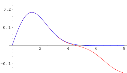
Both eqs. (19) and (20) are displayed in fig. 1. For comparison we display the same quantities of the $\mu$-independent 1RMT. Its rescaled density reads

$$\rho_{1}(\xi)=\frac{\xi}{2}\left[J_{\nu}^{2}(\xi)-J_{\nu+1}(\xi)J_{\nu-1}(\xi)\right]\ (\ =\ {\cal I}^{0}(\xi,\xi)=\rho_{1,0}(\xi)=\rho_{0,1}(\xi)\ )\ ,\$$ (21)

Figure 2: 1RMT at $\nu=0$: the quenched density eq. (21) (green), the exact distribution of the first eigenvalue eq. (22) (blue), and the expansion [18] corresponding to eq. (20) (red).

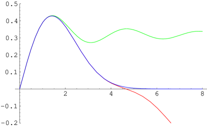
see fig. 2. There we include both the exact distribution of first eigenvalue [17]

$$p_{1}(\xi)=\frac{1}{2}\xi\ e^{-\frac{1}{4}\xi^{2}}\ \ (\nu=0)\ ,$$ (22)

and its corresponding approximation [18].

3.1 Factorisation of correlation functions

In the limit of large chemical potential, $\alpha\gg 1$, the quenched density correlation functions factorise,

$$\lim_{\alpha\gg 1}\rho_{n,k}(\xi_{1,\ldots,n},\zeta_{1,\ldots,k})=\prod_{i}^{n}\xi_{i}\rho_{n,0}(\xi_{1,\ldots,n})\ \prod_{j}^{k}\zeta_{j}\rho_{0,k}(\zeta_{1,\ldots,k})\ ,$$ (23)

where the two factors are given by the $\mu$-independent 1RMT quantities

$$\rho_{n,0}(\xi_{1,\ldots,n})=\rho_{0,n}(\xi_{1,\ldots,n})=\det_{i,j}[{\cal I}^{0}(\xi_{i},\xi_{j})]\ .$$ (24)

This follows from the vanishing of the upper right corner in the determinant eq. (12) when $\alpha$ is large: the corresponding microscopic kernel $M_{N}$ converges to the weight in this limit

$$\lim_{\alpha\gg 1}\left({\cal I}^{-}(\xi,\zeta)-\frac{I_{\nu}\left(\frac{\xi\zeta}{\alpha^{2}}\right)}{\alpha^{2}}e^{-\frac{\xi^{2}+\zeta^{2}}{2\alpha^{2}}}\right)=0\ ,$$ (25)

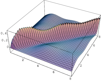
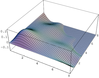
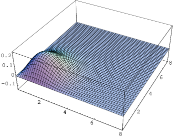
keeping $\xi/\sqrt{\alpha}$ finite. Thus the density from our example eq. (19) factorises, as is shown in fig. 3 left. The deeper reason for the limit eq. (25) will become clearer in the next subsection 3.2.

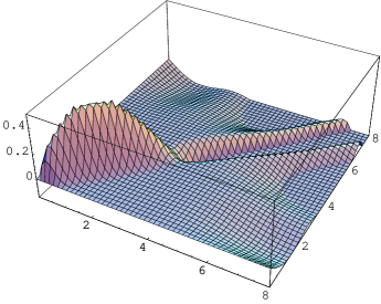
The factorisation of the densities leads to factorised gap probabilities and individual eigenvalue distributions as well, as follows from eq. (14):

Figure 3: Factorisation of the quenched density $\rho_{1,1}(s,t)$: eq. (19) at $\nu=0$ and $\alpha=4.318$ (top left) vs. the factorised eq. (23), using eq. (21) (bottom left). The corresponding approximate individual eigenvalue distribution $p_{1,1}(s,t)$ eq. (20) for the same values (top right) vs. the factorised exact result eq. (28) using eq. (22) (bottom right).

$$\lim_{\alpha\gg 1}E_{k,l}(s,t) = \left(\sum_{i=0}^{N-k}\frac{(-)^{i}}{i!}\int_{0}^{s}dx_{1}\ldots dx_{k+i}\ \rho_{k+i,0}^{(0)}(x_{1},\ldots,x_{k+i})\right)$$ (26)

$$\times\left(\sum_{j=0}^{N-l}\frac{(-)^{j}}{j!}\int_{0}^{t}dy_{1}\ldots dy_{l+j}\ \rho_{0,l+j}^{(0)}(y_{1},\ldots,y_{l+j})\right)$$

$$= E_{k}(s)E_{l}(t)$$

Differentiating twice as in eq. (15) we get

$$\frac{\partial^{2}E_{k,l}(s,t)}{\partial s\partial_{t}}=\frac{\partial E_{k}(s)}{\partial s}\frac{\partial E_{l}(t)}{\partial_{t}}=k!(p_{k}(s)-p_{k+1}(s))\ l!(p_{l}(t)-p_{l+1}(t)),$$ (27)

and thus from comparing to eq. (15)

$$p_{k,l}(s,t)=p_{k}(s)p_{l}(t)\ .$$ (28)

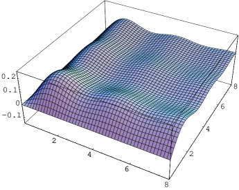
The 1RMT quantities on the right hand side are now explicitly known, without approximations. The comparison in 3D is given in fig. 3 right. In order to check the convergence of eq. (20) we can cut the 3D plot and compare to the exact factorised result, as shown in fig. 4.

Figure 4: 2D cut of fig. 3 top right at $s=1.5$ (red) vs. the exact factorised distribution eq. (28) (blue).

3.2 Factorisation of the weight function

In this section we show that the bi-orthogonal polynomials for the non-Gaussian weight eq. (7) can be constructed in terms of orthogonal polynomials with Gaussian weight. Our discussion follows closely appendix B of [14]. Suppose we have two sets of ordinary orthogonal polynomials

$$\int dx~{}w_{1}(x)~{}P_{k}(x^{2})~{}P_{l}(x^{2}) = f_{k}\delta_{k,l}$$

$$\int dy~{}w_{2}(y)~{}Q_{k}(y^{2})~{}Q_{l}(y^{2}) = g_{k}\delta_{k,l}~{},$$ (29)

with weights $w_{1,2}$ and norms $f_{k}$ and $g_{k}$ respectively. Then it follows that these polynomials are bi-orthogonal with respect to the weight

$$w(x,y) \equiv w_{1}(x)~{}w_{2}(y)~{}\sum_{k=0}^{\infty}~{}\frac{h_{k}}{f_{k}g_{k}}~{}P_{k}(x~{}^{2})~{}Q_{k}(y^{2})~{}.$$ (30)

In our quenched case we can simply choose the ordinary Laguerre weight and its polynomials,

$$w_{1}(x) = w_{2}(x)\ =\ x^{2\nu+1}e^{-\frac{N}{1+\mu^{2}}x^{2}}$$

$$P_{k}(x^{2}) = Q_{k}(x^{2})\ \sim\ L_{k}^{(\nu)}\left(\frac{N}{1+\mu^{2}}x^{2}\right).$$ (31)

The identity that allows to link the Laguerre weight and polynomials to the non-Gaussian weight eq. (7) is given by

$$w(x,y) = (xy)^{\nu+1}~{}e^{-\frac{N(1+\mu^{2})}{4\mu^{2}}(x^{2}+y^{2})}~{}I_{\nu}\left(\frac{1-\mu^{2}}{2\mu^{2}}Nxy\right)$$

$$= 4\mu^{2}\frac{(N(1-\mu^{2}))^{\nu}}{(1+\mu^{2})^{2\nu+1}}(xy)^{2\nu+1}e^{-\frac{N}{1+\mu^{2}}(x^{2}+y^{2})}$$

$$\times\sum_{n=0}^{\infty}\frac{n!(1-\tau)^{n}}{(n+\nu)!}L_{n}^{(\nu)}\left(\frac{N}{1+\mu^{2}}x^{2}\right)L_{n}^{(\nu)}\left(\frac{N}{1+\mu^{2}}y^{2}\right),$$

satisfying eq. (30). The Bessel transforms eq. (9) then simply result into the wave functions

$$\chi_{k}(y) = \int dx~{}w(x,y)~{}P_{k}(x^{2})\ \sim\ y^{2\nu+1}e^{-N\frac{N}{1+\mu^{2}}y^{2}}L_{k}^{(\nu)}\left(\frac{N}{1+\mu^{2}}y^{2}\right)\!.\$$ (33)

All the kernels can now be easily written in terms of Laguerre polynomials and their norms, and we refer to [14] for details. Finally let us reconsider the upper left block in eq. (12). Due to the above identity eq. (3.2) we obtain

$$w(x,y)-M_{N}(x,y)~{}=~{}w_{1}(x)~{}w_{2}(y)~{}\sum_{k=N}^{\infty}~{}\frac{h_{k}}{f_{k}g_{k}}\ P_{k}(x^{2})\ Q_{k}(y^{2}).$$ (34)

Thus naively taking the limit $N\to\infty$ we would expect the right hand side to vanish. However, in the limit eq. (17) this is not the case, and we instead obtain $M_{N}(x,y)\to{\cal I}^{-}(\xi,\zeta)$. Only in the limit of large $\alpha\gg 1$ limit the integral in ${\cal I}^{-}$ extends to $\infty$ in the new variables $\xi/\sqrt{\alpha}$, making it converge to the weight (see eq. (25)). This explains the factorisation in this limit, illustrating the subtlety of the large-$N$ limit (that is distinguished into weak and strong non-Hermiticity for real $\mu$).

Acknowledgements:

I would like to thank the organisers for their generous hospitality during this very stimulating workshop. It is a pleasure to thank F. Basile, P. Damgaard, J. Osborn and K. Splittorff with whom the results have been obtained that are covered in this talk. This work was supported by EPSRC grant EP/D031613/1 and EU network ENRAGE MRTN-CT-2004-005616.

References

- [1] G. Akemann, Int. J. Mod. Phys. A 22 (2007) 1077.
- [2] K. Splittorff and J. J. M. Verbaarschot, arXiv:0710.0704 [hep-th].
- [3] K. Splittorff and J. J. M. Verbaarschot, Nucl. Phys. B 683 467 (2004) [hep-th/0310271].
- [4] J. C. Osborn, Phys. Rev. Lett. 93, 222001 (2004) [hep-th/0403131].
- [5] G. Akemann, J. C. Osborn, K. Splittorff and J. J. M. Verbaarschot, Nucl. Phys. B 712 (2005) 287 [hep-th/0411030];
- [6] G. Akemann, J. Bloch L. Shifrin and T. Wettig, PoS(Lattice2007)244.
- [7] K. Splittorff and J. J. M. Verbaarschot, Phys. Rev. Lett. 98 (2007) 031601 [hep-lat/0609076]; Phys. Rev. D75 (2007) 116003 [hep-lat/0702011].
- [8] G. Akemann and T. Wettig, Phys. Rev. Lett. 92 (2004) 102002 {Erratum-ibid. 96 (2006) 029902} [hep-lat/0308003]; J. C. Osborn and T. Wettig, PoS (LAT2005) 200 [hep-lat/0510115]; J. Bloch and T. Wettig, Phys. Rev. Lett. 97 (2006) 012003 [hep-lat/0604020].
- [9] K. Splittorff and B. Svetitsky, Phys. Rev. D75 (2007) 114504 [hep-lat/0703004].
- [10] F. Basile, G. Akemann, archive/0710.0376 [hep-th].
- [11] J. Gasser and H. Leutwyler, Phys. Lett. B188 (1987) 477.
- [12] D. Toublan and J.J.M. Verbaarschot, Nucl. Phys. B603 (2001) 343 [hep-th/0012144].
- [13] P. H. Damgaard, U. M. Heller, K. Splittorff and B. Svetitsky, Phys. Rev. D 72 (2005) 091501 [hep-lat/0508029]; P. H. Damgaard, U. M. Heller, K. Splittorff, B. Svetitsky and D. Toublan, Phys. Rev. D 73 (2006) 074023 [hep-lat/0602030]; Phys. Rev. D 73 (2006) 105016 [hep-th/0604054].
- [14] G. Akemann, P. H. Damgaard, J. C. Osborn and K. Splittorff, Nucl. Phys. B766 (2007) 34 [hep-th/0609059].
- [15] T. DeGrand and S. Schaefer, PoS(Lattice2007)069; archive/0708.1731v1 [hep-lat].
- [16] G. Akemann and P. H. Damgaard, PoS(Lattice2007)166, arXiv:0709.0484v1 [hep-lat].
- [17] S. M. Nishigaki, P. H. Damgaard and T. Wettig, Phys. Rev. D58 (1998) 087704 [hep-th/9803007];
- [18] G. Akemann and P. H. Damgaard, Phys. Lett. B583 (2004) 199 [hep-th/0311171].