Pair-distribution functions of two-temperature two-mass systems: Comparison of MD, HNC, CHNC, QMC and Kohn-Sham calculations for dense hydrogen

Abstract

Two-temperature, two-mass quasi-equilibrium plasmas may occur in electron-ion plasmas, nuclear-matter, as well as in electron-hole condensed-matter systems. Dense two-temperature hydrogen plasmas straddle the difficult partially-degenerate regime of electron densities and temperatures which are important in astrophysics, in inertial-confinement fusion research, and other areas of warm dense matter physics. Results from Kohn-Sham calculations and QMC are used to benchmark the procedures used in classical molecular-dynamics simulations, HNC and CHNC methods to derive electron-electron and electron-proton pair-distribution functions. Then, nonequilibrium molecular dynamics for two-temperature, two-mass plasmas are used to obtain the pair distribution. Using these results, the correct HNC and CHNC procedures for the evaluation of pair-distribution functions in two-temperature two-mass two-component charged fluids are established. Results for a mass ratio of 1:5, typical of electron-hole fluids, as well as for compressed hydrogen are presented.

I Introduction

The study of hot strongly-coupled dense charged fluids is a difficult task, especially near the regime of or molecular and atomic speciesceperleyH , or excitons in electron-hole plasmas. The system is better understood for fully ionized systems, such as hydrogen, in the form of free electrons and protons, and fully-ionized electron-hole condensates. In fact, considerable headway has been made using methods based on density-functional theory (DFT), even for plasmas with multiple states of ionization. DFT methods have been used with molecular-dynamics based approacheskwon ; dejarlais ; mazevet , as well as within multi-component integral-equation approaches pdw95 ; ilciacco . Equilibrium properties of plasmas, as well as their linear transport properties, have been successfully studied in these papers, and excellent agreement between the molecular-dynamics based DFT and integral-equation based DFT has been found lvm .

On the other hand, laser-produced plasmas are initially formed as two-temperature plasmas, where the electrons have absorbed the laser energy and have self-equilibrated to some “electron temperature” $T_{e}$, while the ions remain cool, at some temperature $T_{i}$, with $T_{i}<T_{e}$. The opposite situation arises in shock-wave generated plasmas, where the ions absorb the shock energy and $T_{i}>T_{e}$. Such two-temperature plasmas also occur in astrophysical settings, affecting the time of termination of synthesis of light-nuclei to occur at different stages of cooling of the electronsastrop , and influencing the Coulomb nuclear-tunneling ratesdewitt . The possibility of such well-defined two-temperature plasmas is largely a result of the extreme mass ratio $m_{i}/m_{e}\geq 1836$ between ions and electrons. Similar, but less well defined situations can arise in electron-hole plasmas, where the masses are of the same order of magnitude (e.g, the electron and hole masses in GaAs are 0.067$m_{e}$ and 0.34$m_{e}$ respectively, with an electron-hole mass ratio of $\sim 5$). GaAs is a direct bandgap material, and electron-hole plasmas are more easily studied in indirect-gap systems like Si where the density-of states mass ratio is $\sim 3$. The simulation of such systems at two temperatures, using quantum Monte-Carlo methods is at present unavailable, even in regimes of densities and temperatures where bound states (or exciton formation in electron-hole systems) do not exist. Thus it is natural to look for analytical methods based on integral-equation techniques which are computationally simple and physically insightful. However, although $T_{e},\,T_{i}$ define the temperatures of each subsystem and the pair-distribution functions (PDFs) $g_{ee}$ and $g_{ii}$, the ‘temperature’ $T_{ei}$ entering into the cross-correlations $g_{ei}$, as well as the the effects of electron spin, exchange etc., relevant to two-temperature systems need to be clarified. In this context we use $T_{ee}=T_{e}$, $T_{ii}=T_{i}$, and $T_{ei}$ to refer to the electron-, ion-, and electron-ion temperatures as they enter independently into the Ornstein-Zernike (OZ) and hypernetted chain (HNC) equations. In fact, some authorsseuf have proposed to modify the well-established OZ equations in dealing with two-temperature (2T) two-mass (2M) systems.

The objective of this paper is to study such 2T-2M plasmas using results from molecular-dynamics (MD)mc , HNChncref , classical-map HNC (CHNC)prl1 ; prb3d , quantum Monte Carlo (QMC)mc and Kohn-Sham (KS)ilciacco methods to establish the proper implementation of quantum effects and 2T, 2M situations in simulation studies. One of our main interests would be uniform hydrogenic plasmas free of bound states, in the regime of warm-dense matter.

II Theoretical Methods

A system of classical particles, e.g., hard-spheres or Lennard-Jones fluids, or classical ions in a uniform neutralizing background, can be studied completely using the method of molecular dynamics (MD) where the classical equations of motion are integrated numerically, for a sufficiently large number of particles contained in a simulation box. It has been found that the particle distribution functions, e.g., the pair-distribution function (PDF) $g_{ij}(r)$ (where $i,j$ specify the species, spin etc.), obtained from MD simulations for charged classical ions can also be accurately reproduced via suitable integral-equations which are computationally very economical and efficient. The pair-potentials, quantum corrections etc., needed to simulate systems with ions and electrons, or purely electron systems (with a uniform neutralizing background) will be discussed in this section. First, we compare the usual HNC approximation with the CHNC method. Then, these results are compared with a full quantum (Kohn-Sham) calculation; these results are then used to determine the effective diffractive interaction used in the CHNC method. Finally, we discuss how the CHNC can be extended to “classical map molecular dynamics” (CMMD).

II.1 HNC and CHNC methods

The HNC equation and its straight-forward generalizations, coupled with the OZ equation have lead to very accurate results for classical charged-particle interactions. The exact equations for the PDFs are of the form:

$$g_{ij}(r)=e^{-\beta_{cf}\phi_{ij}(r)+h_{ij}(r)-c_{ij}(r)+B_{ij}(r)}$$ (1)

Here $\phi_{ij}(r)$ is the pair potential between the species $i,j$. If the bridge function $B_{ij}(r)$ is set to zero we have the HNC approximation. Then, given the temperature $T=1/\beta$, the particle densities $n_{i}$, and the pair-potentials $\phi_{ij}(r)$, the pair-correlation function $h_{ij}(r)$ and the direct correlation function $c_{ij}(r)$ can be self-consistently obtained via the HNC and OZ equations, which have the form

$$h_{ij}(r)=c_{ij}(r)+\sum_{s}n_{s}\int d{\bf r}^{\prime}h_{is}(|{\bf r}-{\bf r}^{\prime}|)c_{sj}({\bf r}^{\prime}).$$ (2)

This method already fails for strictly attractive potentials. Thus, in simulations of electron-proton systems, $\phi_{ep}(r)$ has to be replaced by effective-potentials which attempt to incorporate quantum diffraction effects Jones . Even with purely repulsive potentials, classical simulations fail to incorporate Fermi or Bose statistics which begin to manifest as the density is increased and the temperature is lowered. A well established means of incorporating quantum effects is to derive integral equations from correlated-determinantal wavefunctions, as done in the Feenberg approachfeenberg ; lantto . The resulting integral equations are very daunting, and in fact, not easy to use. Quantum Monte-Carlo (QMC) itself may be considered as an adaptation of the Feenberg-functional to generate a statistical measure for the stochastic algorithms used in MD. An alternative approach, using Feynman paths instead of classical trajectories, provides another class of simulation techniques. However, these quantum simulation methods become computationally extremely heavy. Such methods are best suited for the establishment of bench-mark results, and for the “calibration” of other methods which contain approximation schemes. In fact, the QMC techniques have been most useful in providing the “exchange-correlation” potentials $V_{xc}(r)$ needed in the Kohn-Sham density-functional theory (DFT) equations. While DFT is itself exact, one has to use results from QMC and such microscopic methods to model the unknown $V_{xc}(r)$. Given the $V_{xc}$, the inhomogeneous density distribution around a given particle can be calculated, and the pair-distribution is deduced from it.

The method followed here is to exploit the well established Kohn-Sham equations as the reference calculation, and determine the effective potentials to be used in the classical simulations of 2T and 2M systems. To this end we present comparisons of Kohn-Sham calculations of $g_{ep}(r)$ for H-plasmas with available QMC results to mutually validate these methods. Another theoretical tool we use is the “classical-map HNC”, i.e., CHNC equations which incorporate quantum effects including Fermion statistics via effective potentials and effective temperatures. The CHNC has been extensively tested via comparisons with QMC results in 2-D and 3-D electron systems, and shown to provide excellent agreement, even at the extreme quantum limit of zero temperatureprl1 ; prl2 . CHNC uses a “quantum temperature” $T_{q}$, which depends on the Fermion density. If the physical temperature of the quantum fluid is $T$, the distribution functions are obtainedprl1 from a classical fluid at the temperature $T_{cf}$ such that:

$$T_{cf}=\sqrt{T^{2}+T_{q}^{2}}.$$ (3)

The temperature $T_{q}$ is defined to be such that the classical Coulomb fluid has the same exchange-correlation energy as the quantum fluid [prl1, ]. DFT assures us that only the true density distribution possesses the true exchange-correlation energy. Thus, the charge distributions, i.e., the PDFs obtained from CHNC are found to be in excellent agreement with those from Monte-Carlo simulations of 2D and 3D systems. This agreement is obtained by including the exchange-hole of parallel-spin electrons as an effective potential, called in CHNC the Pauli exclusion potential $P_{ij}(r)$. Clearly, this is zero if $i\neq j$. For $i=j=\parallel$ spins, the potential $P_{ij}(r)$ is such that the non-interacting PDFs, i.e., $g_{ij}^{0}(r)$ are correctly recovered from the integral equationslado . Thus, using atomic units where $|e|=\hbar=m_{e}=1$, the effective pair potentials $\phi_{ij}(r)$ are of the form:

$$\phi_{ij}(r) = P_{ij}(r)+V^{c}_{ij}(r)$$ (4)

$$V^{c}_{ij}(r) = z_{i}z_{j}(1-e^{-k_{ij}r})/r$$ (5)

Here $z_{e}=-1,\,z_{p}=1$ and $k_{ij}$ is a cut-off ’momentum’ defining a diffraction correction allowing for quantum effects. In the simplest formulation $k_{ij}$ is the thermal de Broglie momentum given by:

$$k_{ij} = k^{dB}_{ij}=(2\pi\,m_{ij}T_{ij})^{1/2}$$ (6)

$$m_{ij} = m_{i}m_{j}/(m_{i}+m_{j})$$ (7)

The temperatures $T_{ij}$ entering into the HNC equations for the $g_{ij}(r)$ are given by:

$$T_{ij}/m_{ij}=T_{i}/m_{i}+T_{j}/m_{j}.$$ (8)

The large mass of the proton ensures that the diffraction correction, as well as the $T_{q}$, is negligible for the proton-proton scattering process. A more complete approach to determining $k_{ij}$ is to solve the corresponding Kohn-Sham equation for the two particles in the Kohn-Sham potential of the medium, and matching the $k_{ij}$ so that the quantum and classical values of the PDF at contact are in agreement.

The Pauli exclusion potential is usually determined by inverting the HNC equations applied to the exactly known non-interacting quantum PDFs $g^{0}_{ii}(r)$ of the uniform electron fluid. Here $i$ runs through $e\uparrow,e\downarrow$, i.e., a spin-resolved, two-component electron system is used. If $i\neq j$, $P_{ij}=0$. In the absence of strong magnetic fields, the spin-resolution is not needed in warm dense systems. Treating the electrons as a spin-averaged one-component subsystem simplifies the simulations. Due to the non-linearity of the inversion of the HNC relations given in Eqs. 9, the Pauli exclusion potential for paramagnetic electrons is not a simple average of the Pauli exclusion potentials of the spin-resolved cases. The corresponding Pauli potential $P_{e}(r)$ has to be extracted directly from the averaged $g^{0}_{ee}(r)$. Thus we have, for the spin-resolved and -unresolved cases:

$$\beta P_{ii}(r) = -\ln[g_{ii}^{0}(r)]+N_{ii}^{0}(r),$$ (9)

$$\beta P_{e}(r) = -\ln[\{g_{ii}^{0}(r)+1\}/2]+N^{0}_{ii}/2$$ (10)

$$N_{ii}^{0}(r) = h_{ii}^{0}(r)-c_{ii}^{0}(r).$$ (11)

A bridge term $B_{ij}(r)$ is used to correct the HNC for multi-particle effects poorly rendered by HNC. Such bridge corrections are found to be very significant in the 2D electron fluidprl2 , but not for 3D electrons at densities and temperatures considered in this study.

The CHNC differs from HNC in the use of the Pauli potentials and the quantum temperature $T_{q}$ when treating quantum fluids. Also, the pair-potentials used in HNC have been constructed to agree with KS-charge profiles (see below). Hence any insights obtained for the two-temperature two-mass HNC can be easily transfered to the CHNC. The two-temperature electron-ion plasma was discussed in a formal analysis by Boercker and Morebm , using a product form for the partition function. However, no comparisons of their results with actual simulations are available. The more general two-temperature two-mass HNC type equations have been discussed, most recently by Seuferling et al.seuf . Using an analysis based on the Bogoliubov-Born-Green-Kirkwood-Yvon (BBGKY) hierarchy as well as some factorization assumptions, the authors of Ref. [seuf, ] have proposed modified OZ type equations for 2T-2M plasmas. While their formulae reduce to the usual OZ equations, viz., Eq. 2, for the $m_{a}>>m_{b},\;T_{a}=T_{b}$, the case $m_{a}=m_{b},\;T_{a}=T_{b}$ is not correctly recovered. The results presented in our study imply that the usual OZ equations hold in all cases, as long as the correct mass-dependent $T_{ij}$, Eq. 8 is used in 2T-2M systems.

II.2 The Kohn-Sham reference calculation

Kohn-Sham theory at finite temperaturesilciacco states that the true one-particle density distribution of the system subject to an external potential is such that the free energy of the system is minimized. This theorem holds rigorously for a system in equilibrium and we use it to derive distribution functions by considering the inhomogeneous electron distribution around a proton in the plasma. Let $n(r)$ and $\rho(r)$ be the electron and proton charge densities around the proton at the origin. These tend to the average densities $\bar{n}=\bar{\rho}$ far away($r\to\infty$) from the proton at the center; then,

$$g_{ep}(r)=n(r)/\bar{n}.$$ (12)

Instead of using a two-component DFT procedure, we make the further approximation, well established in practice, where the proton subsystem is replaced by a uniform positive background with a cavity, viz., a Wigner-Seitz sphere of radius $r_{s}=\left[3/(4\pi\bar{n}\right]^{1/3}$. The positive charge scooped out to form the cavity is placed as a point charge at the origin, and forms the central proton. The finite-temperature Kohn-Sham equation is a consequence of the Euler equation for the stationary property of the free energy under functional derivation with respect to the electron-density distribution, viz.,

$$\frac{\delta F([n(r)])}{\delta n(r)}=0.$$ (13)

A standard Kohn-Sham type analysis now leads to the equation:

$$[-\nabla^{2}/2+Z/r-V_{ks}(r)]\psi_{\nu}(r)=\epsilon_{\nu}\psi_{\nu}(r),$$ (14)

where

$$V_{ks}(r) = V_{p}(r,n(r))+V_{xc}(r,n(r),T_{e})$$

$$n(r) = \sum_{\nu}|\phi_{\nu}(r)|^{2}f(\epsilon_{\nu}/T_{e}).$$

Here

$$V_{P}(r,n(r))=\int d{\bf r^{\prime}}n(r^{\prime})/|{\bf r}-{\bf r^{\prime}}|$$

is the Poisson potential of the electron distribution $n(r)$. This distribution is evaluated self-consistently from the Kohn-Sham wavefunctions $\psi_{\nu}(r),\;\nu=n,l,m$, energy $\epsilon_{\nu}$, with the occupation factor given by the Fermi function $f(\epsilon/T_{e})$. The potential due to the proton at the origin is $Z/r$, with $Z=1$, and $V_{xc}(r,n(r),T_{e})$ is the finite-temperature Kohn-Sham exchange-correlation potentialprb3d which depends self-consistently on the charge profile $n(r)$. This is evaluated using the local-density approximation (LDA), unlike in CHNC where a fully non-local $V_{xc}(r)$ is evaluated via a coupling-constant integration over the $g_{ee}(r)$. The Kohn-Sham procedure uses only $n(r)=\bar{n}g_{ep}(r)$, and does not provide a $g_{ee}(r)$. Since this problem contains only one proton, there is no proton temperature in the theory. However, due to the large mass of the proton, and due to the exclusion of other protons by the central proton (modeled by the Wigner-Seitz cavity), the value of $g_{ep}(r)$ at $r\to 0$ given by the Kohn-Sham calculation is expected to be a valid estimate for the full electron-proton plasma. In fact, in the two-temperature electron-proton plasma, $T_{ep}$ of Eq. 8 reduces to $T_{ee}$, as in the Kohn-Sham calculation, since $m_{p}>>m_{e}$. That this one-proton Kohn-Sham calculation correctly reproduces the $g_{ep}(r)$ of the plasma, even at very low temperatures, is seen from the comparisons given in Fig. 1, where the path-integral Monte Carlo (PIMC) PDFs for hydrogen from the work of Militzer and Ceperleymilicep have been used.

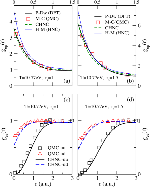
Figure 1: (Online color)Panels (a),(b) present a comparison of the DFT, QMC, CHNC, MD, and HNC calculations of the electron-proton PDF. The last three use the effective potentials of Eq. 15. A quantum temperature $T_{q}$, a Pauli potential and the effctive potentials with $f_{ep}$ different from unity are used in CHNC. The lower panels compare the spin-resolved electron-electron PDfs in the H-plasma, obtained from QMC and CHNC. P-Dw(DFT) and CHNC calculations use the formulations of Dharma-wardana and Perrotilciacco ; prl1 . The QMC (PIMC) is from Militzer and Ceperleymilicep , while the H-M(HNC) follow the MD calculations of Hanson and MacDonaldhanmac using the potentials of Eq. 18.

II.3 The effective electron-proton interaction for classical simulations.

In a classical simulation of an electron-proton plasma, or in a CHNC calculation, the Coulomb interaction $V_{ep}(r)$ appears. This is the attractive classical potential associated with the quantum-mechanical operator $-1/r_{ep}$. It is expected to have the form:

$$V_{ep}(r) = -\left[1-e^{-k_{ep}r}\right]/r$$ (15)

$$k_{ep} = k^{dB}_{ep}f_{ep}$$ (16)

$$k^{dB}_{ep} = \left[2\pi T_{ep}m_{ep}\right]^{1/2}$$ (17)

The thermal de Broglie momentum $k^{dB}$ provides a first approximation to $k_{ep}$. But we choose $k_{ep}$ such that the $g_{ep}(r\to 0)$ generated by the classical procedure (e.g., MD or CHNC) agrees with the $g_{ep}(r\to 0)$ obtained from the Kohn-Sham calculation at the given $r_{s}$ and $T_{e}$. It turns out that the correction factor $f_{ep}$ is quite close to unity for sufficiently high temperatures. Even at $T$=10.77 eV, $r_{s}=1$, i.e., $T/E_{F}$=0.215, $f_{e}$=0.922 and we see from Fig. 1 that the agreement between QMC, DFT, and CHNC is quite good. We have determined the value of $f_{ep}$ as a function of $T_{e},r_{s}$ by matching the CHNC calculation and the Kohn-Sham calculation. In effect, $f_{ep}$ is similar to a pseuodopotential or form factor for the electron-proton interaction. When bound states begin to be formed ($r_{s}>1.8$), the form of $f_{ep}$ becomes more critical, but this problem does not arise within the densities studied here. However, classically, for attractive potentials, dynamical instabilities could occur at any $r_{s}$, $T$ and these have to be controlled using close-approach cutoffs on the potentials, as well as controls on the velocity distribution functions, to maintain the meaning of “subsystem temperatures” which are set to $T_{e}$ and $T_{i}$. Investigation of such instabilities where the velocity distributions do not conform to the two-temperature model is outside the scope of this study.

The electron-electron interaction used in CHNC, and MD simulations, is also a diffraction-corrected Coulomb potential, $V_{ee}(r)$, with $k_{ee}$ being $(2\pi m_{ee}T_{cf})^{1/2}$, with $m_{ee}=m_{e}/2$ and requiring no additional correction factors. This diffraction correction can be derived from the Schrödinger equation describing electron-electron scatteringprl3 .

II.4 Classical-map Molecular dynamics

The HNC method using all three items: (i) diffraction-corrected effective potentials, (ii) the Pauli exclusion potential and (iii) the quantum temperature $T_{q}$, is the CHNC scheme. If the same three items were included in classical molecular dynamics simulations, we have a classical-map-MD scheme (CMMD). The CMMD is superior to CHNC since it automatically includes any bridge corrections, etc. that are not in the HNC scheme. In CMMD the electron temperature would be $T_{cf}$, Eq. 3, as in CHNC. However, since bridge corrections are expected to be negligible in the regime of densities and temperatures considered here, we do not carry out CMMD simulations.

III Results

We first provide comparisons between simple classical MD simulations and HNC calculations of PDFs of 2T-2M systems using the simplest diffraction corrected pair potentials, given by:

$$\phi^{0}_{ij} = z_{i}z_{j}(1-e^{-k^{dB}_{ij}r})/r$$ (18)

$$k^{dB}_{ij} = \left[2\pi m_{ij}T_{ij}\right]^{1/2}$$ (19)

The MD simulations only need the individual subsystem temperatures $T_{ii}$, $T_{jj}$, and no cross-species temperature $T_{ij},i\neq j$ is needed. This is achieved by employing two velocity-scaling thermostats that adjust the electron and ion velocity distributions to have the desired mean values. In contrast, the HNC needs a specification for $T_{ij}$. Seuferling et al.seuf have suggested that the OZ equations also need to be modified. These issues can be tested by comparison with the MD results.

III.1 Two-mass two-temperature systems.

Systems where the two masses $m_{a}$ and $m_{b}$ of the two components $a,b$ are equal cannot produce two-temperature quasi-equilibrium systems unless $V_{ab}$ is, for some reason, extremely different from $V_{bb}$ and $V_{aa}$. Thus two-temperature plasmas may exist for significant times, even when the mass-ratio is of the order of 3-10, as in some solid state electron-hole plasmas where band-structure effects associated with the existence of indirect gaps introduce restrictions on electron-hole recombination. Here we present HNC calculations of the PDFs of plasmas with $m_{b}/m_{a}=5$, and compare them with MD simulations, to establish the correct implementation of HNC and CHNC procedures.

In Fig. 2 we show the PDFs calculated for a two-component system with a mass ratio of 5, using both the HNC with the standard OZ relations and MD. The MD simulations used 300 particles, 40,000 equilibration steps, a time step of 0.02 of the inverse electron-plasma frequency, and data was then accumulated over 120,000 steps using the two thermostats described above. In the HNC calculation, the pair-potentials are given by Eq. 18, and the cross-species temperature is as in Eq. 8. This simple HNC-OZ procedure is in very good agreement with MD, both for the equilibrium and non-equilibrium (two-temperature) cases, and we conclude that the additional procedures proposed by Seuferling et al.seuf in their Eq. (37) are not needed. That is, our results show that a modified OZ equation is not necessary. The comparison between the HNC and the MD establishes the correctness of the basic HNC procedures even in the quasi-equilibrium case where the formal derivation of the HNC equations becomes an open question. However, once the correct HNC procedure is established, the calculations for the quantum two-temperature two-mass system can be carried out using the CHNC, with the same temperature assignments $T_{ij}$ extended to include the quantum temperatures $T_{q}$, and the Pauli potentials.

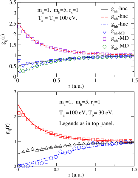
Figure 2: (Online color)The upper panel shows the PDFs for a two-component ($a,b$) system at a temperature $T_{a}=T_{b}=100$ eV, $r_{s}=1$, the masses $m_{a},\,m_{b}$ being 1 and 5. The component $a$ electron like, while $b$ is hole-like, i.e., positively charged. Lower panel shows the two-temperature two-mass case, with $T_{b}$ lowered to 30 eV. In both cases the PDFs $g_{ij}(r)$ calculated using the standard HNC and the OZ equation, Eq. 2 agree well with the MD results using the same input potentials as in HNC.

III.2 Electron-proton systems in thermal equilibrium

The simple diffraction corrected potentials, Eqs. 18 were used by Hanson and MacDonald in H-plasma simulationshanmac . Their PDFs can also be generated using the simple HNC equations if the above $\phi_{ij}(r)$ are used. Hence, in Fig. 1 we have labeled the corresponding $g_{ep}(r)$ as H-M(HNC,MD). The PDFs obtained from the DFT calculation, using Eq. 14, as implemented in the codes by Perrot and Dharma-wardanadpcodes , as well as the PIMC results of Militzer and Ceperley are also shown, to establish that these two first-principles methods are in excellent agreement. Here we note that the CHNC results for $g_{ep}$ and also the spin-resolved $g_{ee}$ are in excellent agreement with the QMC PDFs. To obtain this agreement, the CHNC uses the slightly modified diffraction parameter $k_{ep}=f_{ep}k^{dB}_{ep}$ with $f_{ep}$=0.922 and 0.965 at $r_{s}$=1 and 1.5 respectively, as obtained by matching the contact value of the CHNC $g_{ep}$ to the value from the KS calculation. The MD-HNC using the Hanson-MacDonald approach leads to a large value of $g_{ep}$ at $r\to 0$, while the $g_{ee}$ (not shown in the figure) are in strong disagreement. The agreement between QMC and CHNC shown in Fig. 1 holds even better at higher temperatures, and this justifies our use of the CHNC and Kohn-Sham results as the reference calculations when QMC results are not available.

III.3 Two-temperature electron-proton systems

In this sub-section we compare classical two-temperature H-plasmas and show that the temperature $T_{ep}$ that appears in the cross-species HNC equation is indeed the electron temperature $T_{ee}$, as in Eq. 6, for the limit $m_{p}>>m_{e}$. Thus, we use the same $T_{ep}$ in the CHNC, to include the quantum corrections and compute $g_{ij}(r)$. In Fig. 3 we show the cross-species (electron-proton) PDF for a hydrogen plasma with $T_{e}=100$ eV, $r_{s}=1$, for the four cases: $T_{i}=100,\,60,\,30$ and 10. From panel (a) we see that the classical procedures (HNC and MD) using the simplest set of $\phi_{ij}(r)$, Eq. 18, overestimate the $g_{ep}$ in comparison to the Kohn-Sham (DFT) estimate. In panels (b-d) we have two-temperature plasmas, and the MD calculation (which needs only $T_{e},T_{i}$) is closely reproduced by the HNC if $T_{ep}$ is set to $T_{e}$. In panel (b) we show that the choice $T_{ep}=(T_{e}+T_{p})/2$ in the HNC is clearly inapplicable if the system is entirely specified by $T_{e},\,T_{p},\,$ and $r_{s}$.

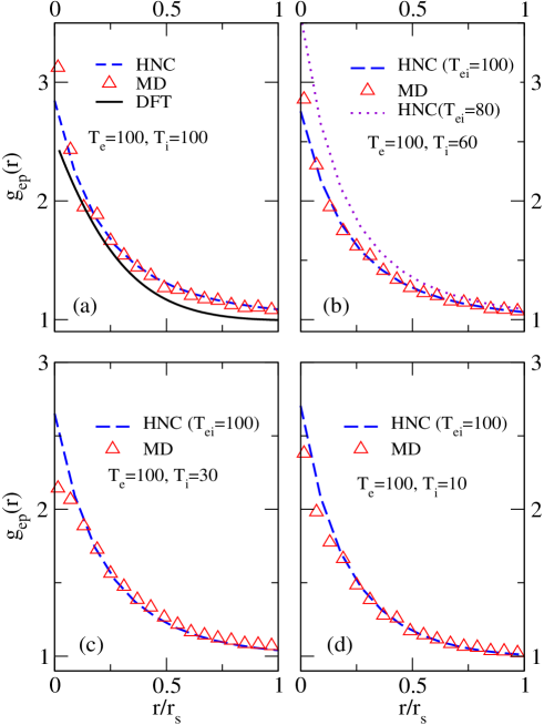
Figure 3: (Online color) Dense hydrogen: Panel (a) compares HNC and MD $g_{ep}(r)$ using the simplest set of classical potentials (Eq. 18). The DFT PDF shows that the classical potentials are an overestimate. In panels (b-d) we use the same classical potentials to establish that the temperature $T_{ep}$ needed in the HNC is indeed $T_{e}$ if HNC and MD are to agree for two-temperature electron-proton systems.

As seen from Fig. 3, quantum effects may significantly modify the PDFs even when the electrons are at 100 eV.

Thus, in Fig. 4, we present CHNC calculations for a two-temperature plasma with $T_{e}=100,T_{i}=30$ at the density $r_{s}=1$. The top panel shows that the proton-proton PDF calculated from the quantum procedure (using CHNC) is more strongly coupled than in the classical (using HNC) $g_{pp}$. The stronger e-p interaction in the classical system, as shown in the enhanced $g_{ep}$, leads to greater screening, weakening the ion-ion interaction. The lower panel shows the spin-resolved e-e PDFs, labeled $g_{uu},g_{ud}$ obtained from CHNC, and the classical $g_{ee}$ obtained from HNC. The CHNC correctly incorporates the exclusion effects via the Pauli potential, Eq. 9.

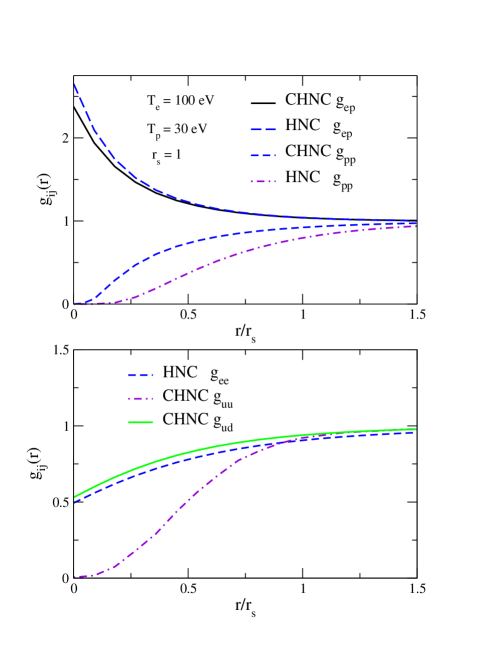
Figure 4: (Online color)The upper panel shows the e-p and p-p PDFs for an electron-proton plasma with $T_{e}=100$eV, $T_{p}=30$eV, $r_{s}=1$, calculated using HNC and CHNC. The lower panel shows the e-e PDFs, where the HNC does not incorporate the effects of the exclusion principle. The CHNC $g_{uu}$ and $g_{ud}$ refer to spin parallel and antiparallel PDFs respectively.

III.4 The electron-proton PDF and Pauli exclusion effects

The electron-proton pair distribution function is mainly determined by the e-p interaction which is spin-independent. However, once an electron is correlated with a proton, the correlation of that electron with other electrons would be affected by Pauli exclusion effects associated with the electron spin. In the CHNC and CMMD schemes, the effect of the Pauli principle are incorporated as a potential, Eq. 9, between parallel-spin electrons. This potential is not used in MD and in the pure HNC scheme. Hence the $g_{ee}(r)$ obtained from HNC, shown in the lower panel of Fig. 4(b) is identical for parallel and anti-parallel PDFs. However, Fig. 4(a) shows that the $g_{ep}$ obtained by the full CHNC, inclusive of the Pauli potential, $f_{ep}$, and $T_{q}$ features is quite close to the pure-HNC result where $f_{ep}=1$ in the diffraction potentials. At $r_{s}=1$, $T_{q}/E_{F}=0.768$, and hence, when $T_{e}=100$ eV, i.e., $T_{e}/E_{F}=1.9956$, then $T_{q}$ itself is substantial. Thus the larger value of $g_{ep}(r)$ at $r\to 0$ found in the HNC and MD is not due to the Pauli exclusion effects, but due mainly to two reasons: (i)the overestimate contained in the zeroth set of effective potentials where $f_{ep}=1$, and (ii)the use of the physical temperature $T_{e}$ as the effective temperature of the classical electron fluid, while $T_{cf}>T_{e}$ is used in the CHNC. To check these, we have run CHNC calculations where (i) the Pauli potential was switched off while the $T_{q}$, $f_{ep}$ were included; (ii) only the Pauli and $f_{ep}$ were included; (iii) only the Pauli and $T_{q}$ were included; and so forth. Such “numerical experiments” enable us to conclude that the Pauli exclusion effect is of relatively low importance for the $g_{ep}(r)$ when $T_{e}$ is 100 eV and $r_{s}=1$.

IV concluding discussion

The simplest classical rendering of quantum plasmas, based on the use of diffraction corrected potentials (Eq. 18) was used with HNC calculations and MD simulations to resolve the ambiguities and difficulties in handling the two-temperature, two-mass system. We conclude that the modifications to the OZ equations proposed by Seuferling et al.seuf ., are not needed. The classical mapping of quantum systems to the HNC equations, as used in the CHNC was confirmed by comparisons with Kohn-Sham DFT calculations as well as with available PIMC results for compressed hydrogen plasmas at finite temperatures. We conclude that the HNC and CHNC, together with the standard OZ equations provide excellent, accurate and simple analytical tools for the investigation of many-particle quasi-equilibrium systems for which direct quantum simulations continue to remain too prohibitive or unfeasible.

References

- (1) K. T. Delaney, C. Pierleoni, D. M. Ceperley. Phys. Rev. Lett. 97, 235702 (2006). C. Pierleoni, D. M. Ceperley, Markus Holzmann. Phys. Rev. Lett. 95, 146402 (2004)
- (2) I. Kwon, L. Collins, J. Kress and N. Troullier, Phys. Rev. E. 54, 2844 (1996)
- (3) M. P. Desjarlais, Phys. Rev. B 68, 64204 (2003);
- (4) S. Mazevet, M. P. Desjarlais, L. A. Collins, J. D. Kress and N. H. Magee, Phys. Rev. E 71, 016409 (2005)
- (5) F. Perrot and M.W.C. Dharma-wardana, Phys. Rev. E. 52 , 5352 (1995)
- (6) Density Functional Theory, Ed. E. K. U. Gross and Dreizler, NATO ASI Series B: Physics 337 (Plenum, NY. 1993)
- (7) M.W.C. Dharma-wardana, Phys. Rev. E. 73, 036401 (2006)
- (8) F. A. Agronyan and R. A. Syunyaev, Astrophysics 27, 413-422; Translated from Astrofizika; 27: No. 1, 131-145 ( 1987)
- (9) A.I. Chugunov, H. E. DeWitt, and D. G. Yakovlev, Phys. Rev. D 76, 025028 (2007)
- (10) P.Seuferling, J. Vogel, and C. Toepffer, Phys. Rev. A 40, 323 (1989)
- (11) D. P. Landau and K. Binder A guide to Monte Carlo simulations in statistical Physics (Cambridge University Press 2005)
- (12) J. M. J. van Leeuwen, J. Gröneveld, J. de Boer, Physica 25, 792 (1959)
- (13) M. W. C. Dharma-wardana and F. Perrot, Phys. Rev. Lett. 84, 959 (2000)
- (14) F. Perrot and M.W.C. Dharma-wardana, Phys. Rev. B, 62, 16536 (2000);
- (15) C. S. Jones and M. S. Murillo, High Energy Density Phys. (doi:10.1016/j.hedp.2007.02.038) (2007).
- (16) E.Feenberg, Theory of Quantum Fluids (Academic, New York 1969)
- (17) L. J. Lantto, Phys. Rev. B 22, 1380 (1980)
- (18) F. Perrot and M. W. C. Dharma-wardana, Phys. Rev. Lett. 87, 206404 (2001)
- (19) F. Lado, J. Chem. Phys. 47, 5369 (1967)
- (20) D. B. Boercker and R. M. More, Phys. Rev A 33 1859 (1986)
- (21) B. Militzer and D. Ceperley , Phys. Rev. Lett. 85, 1890 (2000); B. Militzer, Thesis, (2000), see http://militzer.gl.ciw.edu/diss/diss_militzer.pdf
-
(22)
M. W. C. Dharma-wardana and François Perrot;
http://athens.phy.nrc.ca/ims/qp/codes/chandre/D_P/
access by password obtainable from: chandre.dharma-wardana@nrc-cnrc-gc.ca - (23) J.-P. Hansen, I. R. MacDonald, Phys. Rev. Lett. 41 1379 (1978)
- (24) M.W.C. Dharma-wardana and F. Perrot, Phys. Rev. Lett. 90, 136601 (2003)