Observation of an unexpected hardening in the spectrum of GRB 021206

Abstract

GRB 021206 is one of the brightest GRBs ever observed. Its prompt emission, as measured by RHESSI, shows an unexpected spectral feature. The spectrum has a peak energy of about 700 keV and can be described by a Band function up to 4.5 MeV. Above 4.5 MeV, the spectrum hardens again, so that the Band function fails to fit the whole RHESSI energy range up to 17 MeV. Nor does the sum of a blackbody function plus a power law, even though such a function can describe a spectral hardening. The cannonball model on the other hand predicts such a hardening, and we found that it fits the spectrum of GRB 021206 perfectly. We also analysed other strong GRBs observed by RHESSI, namely GRBs 020715, 021008, 030329, 030406, 030519B, 031027, 031111. We found that all their spectra can be fit by the cannonball model as well as by a Band function.

1 INTRODUCTION

The exact mechanism which produces $\gamma$-ray bursts (GRBs) has not yet been definitively established. Their prompt $\gamma$-ray spectra can be used to distinguish between different models. Several mathematical functions have been used for parametrizing the prompt $\gamma$-ray emission. Most commonly used is the empirical Band function (Band et al., 1993), which is not motivated by a physical model.

There have been attempts to distinguish between spectral models analysing the low energy part of the spectrum. Ghirlanda et al. (2003), Ryde (2004), and more recently Ghirlanda et al. (2007) searched for blackbody components in GRB spectra with varying degrees of success. Preece et al. (2002), using BATSE GRB spectra, tested the synchrotron shock model and conclude that it ”does not account for the observed spectra during the GRB phase”.

Spectral studies above the peak energy are rare, one reason being the poor data quality because of lack of statistics. Combining BATSE and EGRET spectra, González et al. (2003) report a high energy component for GRB 941017. They find a photon index of about 1.0 at energies above 5 MeV.

In this paper we report a high energy component in GRB 021206 (Hurley et al., 2002c, 2003b), observed with the Reuven Ramaty High Energy Solar Spectroscopic Imager RHESSI (Lin et al., 2002). Having a peak energy of about 700 keV, the spectrum of this burst can be described by a Band function from 70 keV up to 4.5 MeV, with a high energy photon index $\beta\approx 3.2$. Above 4.5 MeV, the spectrum hardens again, and can be described with a photon index $\beta^{\prime}\approx 2.2$. This significant hardening around 4.5 MeV can not be described with a Band function. But it seems to differ from the spectral hardening in GRB 941017 as well.

There is one model that fits the entire RHESSI spectrum of GRB 021206: the cannonball model (Dar & de Rújula, 2004; Dado, Dar & de Rújula, 2002, 2003a). The cannonball model predicts a spectral hardening at several times the peak energy with a high energy photon index reaching $\beta\approx 2.1$.

The question immediately arises whether the cannonball model can improve our description of other GRB spectra. The difference between the Band function and the cannonball model arises only at the high energy part of the spectrum, where data usually suffer from low statistics. Therefore, we choose the strongest GRBs registered by RHESSI in the years 2002 to 2004. We find that they all can be fit by the cannonball model as well as by the Band function.

The outline of the paper is the following: We first present shortly the instrument, the GRB selection, the spectrum extraction, and the fit method (§2). In the next section (§3), many spectral functions are given. In §4, the fit results for GRB 020715, GRB 021008, GRB 021206, GRB 030329, GRB 030406, GRB 030519B, GRB 031027, and GRB 031111 are presented. The fits are discussed and, if possible, compared to other measurements. The more general discussion, including an outlook, follows in §5. We end with a short summary in §6.

2 INSTRUMENT AND METHOD

2.1 Instrument

RHESSI is a NASA Small Explorer mission designed to study solar flares in hard X-rays and $\gamma$-rays (Lin et al., 2002). It consists of two main parts: an imaging system and the spectrometer with nine germanium detectors (Smith et al., 2002). The satellite always points towards the Sun and rotates about its axis at $15\,$rpm. The Ge detectors are arranged in a plane perpendicular to this axis.

The shape of the detectors is cylindrical with a height of $\approx 8.5\,$cm and diameter of $\approx 7.1\,$cm, and they are segmented into a thin front ($\approx 1.5\,$cm) and a thick rear segment ($\approx 7\,$cm). Since the shielding of the rear segments is minimal, photons with more than about 25 keV can enter from the side. Above about 50–80 keV, photons from any direction can be observed. Each detected photon is time- and energy-tagged from 3 keV to 2.8 MeV (front segments) or from 20 keV to 17 MeV (rear segments). The energy resolution is $\approx 3$ keV at 1 MeV, and the time resolution is 1 $\mu$s.

The effective area for GRB detection depends on the incident photon energy $E$ and the angle between the GRB direction and the RHESSI axis, the incoming angle $\theta$. Over a wide range of $E$ and $\theta$, the effective area is around 150 cm². The sensitivity drops rapidly at energies below $\approx 50$ keV.

2.2 GRB selection

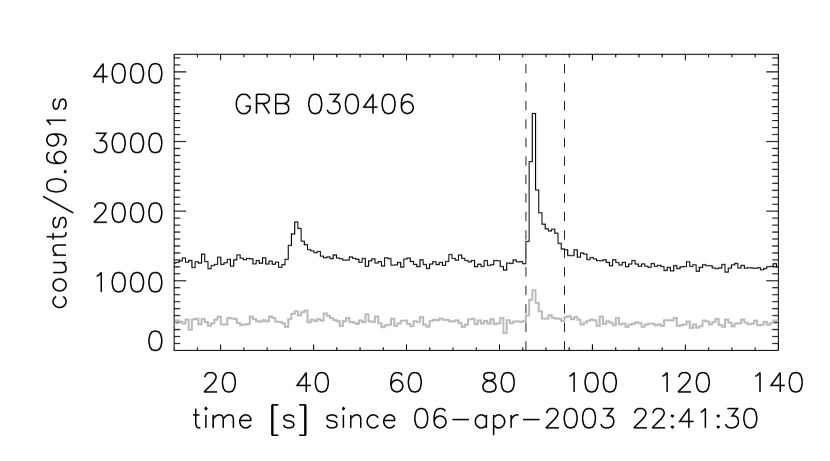
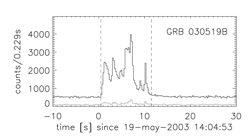
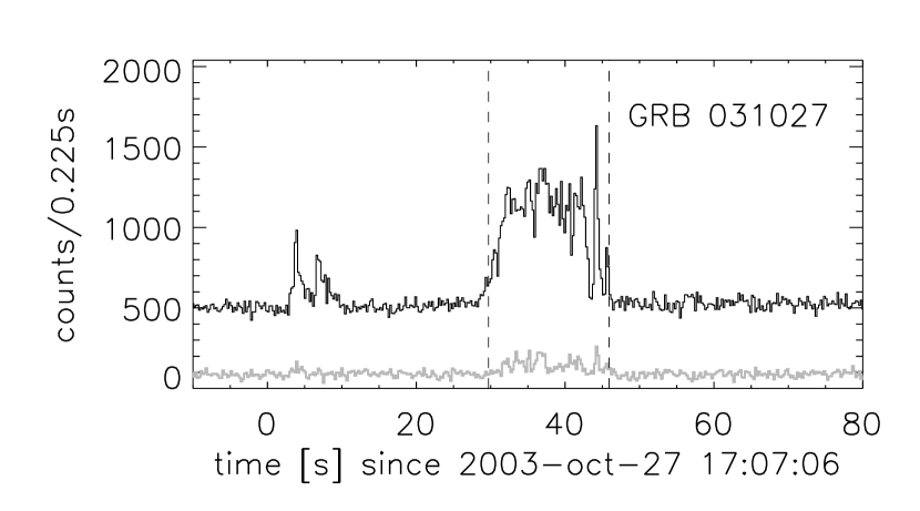
Figure 2: lightcurves for the energy band 20 keV to 3 MeV; black: rear detectors, grey: front detectors; broken vertical lines: time intervals used for spectral analysis.

For this study, we need well observed GRB spectra. We chose GRBs from the years 2002 to 2004, because radiation damage starts to play a role in 2005. The selected GRBs have to be localized by other observations of the same GRB (RHESSI can not measure the incoming angle), because $\theta$ enters into the simulation of the response function. A further requirement was the availability of good background data. And finally, the data storing mode (‘rear decimation’ for onboard memory saving) is not allowed to change during the entire GRB and background time interval. Of all the GRBs meeting these criteria, we chose eight with the best signal-to-background ratio, listed in Table 1 along with their incoming angle $\theta$ and the time intervals used. The lightcurves of these bursts are shown in Figs. 1 and 2.

2.3 Preparation and fit of RHESSI spectra

The method of analysing RHESSI GRB spectra will be described in detail in a separate article (E. Bellm, C. Wigger et al., in preparation).

For each GRB and detector segment, the total spectrum (GRB plus background) during the burst was extracted, as well as the background spectra during two time intervals before and after the burst. The background was linearly (sometimes quadratically) interpolated and subtracted. The exact time intervals are listed in Table 1. Then we added all rear and all front segments, except for detector #2 which is slightly damaged and has a bad energy resolution. Since all GRBs in this study are strong, the observational errors are dominated by the statistical error of the GRB counts, not of the background.

We simulate RHESSI using GEANT3 (CERN, 1993). Knowing the direction of the GRB from other instruments, we simulate RHESSI’s response to photons coming from angle $\theta$. The energy of the incoming photons is simulated as a power law spectrum (i.e. $dN/dE\propto E^{-\gamma_{sim}}$) with typically $\gamma_{sim}=2\,$. This power law simulation is only a rough approximation and is not not intended to represent the intrinsic GRB spectrum, but instead provides simulated data representing RHESSI’s conversion of photons to counts. The true GRB source spectrum is determined via weight factors for the resulting simulated count spectrum, as described below. The upper energy limit of the simulated photon spectrum is typically 30 MeV, in the case of GRB 021206 even 40 MeV or 50 MeV. This is important, because an incoming photon of e.g. 25 MeV may well make a signal of 15 MeV. Rotation angles are generated uniformly, i.e. we compute a RHESSI-spin averaged response function. Since the detector arrangement shows an approximate 120 degree symmetry, the averaging gives good results as long as the analysed time interval is at least one third of the rotation period ($T_{rot}=4\,$s). This was also confirmed by tests.

The output of the simulation is an event list, or rather a hit list, consisting of all signals registered in the Ge detectors. The simulated hit list, having $N_{s}$ entries indexed by the letter $l$, contains the deposited energy ($E^{\mbox{\em\scriptsize det}}_{l}$) as well as the initial photon energy ($E^{\mbox{\em\scriptsize in}}_{l}$). The measured hit list contains only the observed energy.

For spectral fitting, the observed energy histogram is compared with a histogram accumulated from the simulated hit list. More precisely: The measured histogram can be represented by a $k$-element vector $\vec{M}$ with errors $\vec{\sigma}_{M}$, and energy boundaries $E^{b}_{0}$, $E^{b}_{1}$, $E^{b}_{2}$, …, $E^{b}_{k}$. We normalize the histogram $\vec{M}$ to the total number of counts in the fit range: $\vec{m}=\vec{M}/C_{M}$ and $\vec{\sigma}_{m}=\vec{\sigma}_{M}/C_{M}$, where $C_{M}=\sum_{i\in I}M_{i}$ and the sum goes only over the bins included in the fit, i.e. $I=\{i\mid\mbox{bin }i\mbox{ is included in the fit}\}$. The ’theoretical’ histogram $\vec{S}$ is accumulated from the simulated hit list. Each entry is weighted with a factor in order to scale from the simulated power law to the probability density which would be expected, had we actually simulated the GRB source spectrum dN/dE. The $j$th bin contains therefore the weighted sum of all simulated hits with $E^{\mbox{\em\scriptsize det}}_{l}$ belonging to that bin, i.e.:

$$S_{j}=\sum_{l\in L}w_{l}$$ (1)

where $L=\{l\mid E^{b}_{j-1}\leq E^{\mbox{\em\scriptsize det}}_{l}<E^{b}_{j}\}$ and

$$w_{l}=\left(\frac{E^{\mbox{\em\scriptsize in}}_{l}}{E_{piv}}\right)^{\gamma_{sim}}\cdot\frac{dN}{dE}(E^{\mbox{\em\scriptsize in}}_{l})$$ (2)

The first factor in eq. 2 accounts for the spectrum assumed in the simulation and the energy $E_{piv}$ is an arbitrary normalisation. The second factor accounts for the spectrum of the incoming GRB photons. Possible parametrisations of $dN/dE$ are given below in §3. If the GRB spectrum had the same shape as the simulated one, i.e. if $dN/dE=(E/E_{piv})^{-\gamma_{sim}}$, the weights would all be 1 . This method of using weight factors when filling a histogram is common in particle physics, see e.g. Barlow & Beeston (1993). The statistical error of the ’theoretical’ histogram $\vec{S}$ is $\sigma^{2}_{S_{j}}=\sum_{l\in L}w_{l}^{2}$ (§6 of Barlow & Beeston, 1993). As in the case of the measured histogram, the histogram $\vec{S}$ is normalised: $\vec{s}=\vec{S}/C_{S}$ and $\vec{\sigma}_{s}=\vec{\sigma}_{S}/C_{S}$ with $C_{S}=\sum_{i\in I}S_{i}$.

The parameters of the histogram $\vec{S}$ are varied until the minimum of

$$\chi^{2}=\sum_{i\in I}\frac{(m_{i}-fs_{i})^{2}}{\sigma_{m_{i}}^{2}+\sigma_{s_{i}}^{2}}$$ (3)

is found. The factor $f$ accounts for the normalisation between measured and simulated histogram. It is expected to be almost 1, but should be treated as a free fit parameter. For each fit iteration, the histogram $\vec{S}$ is recalculated with different weights (eq. 2).

Since the simulated hit list contains many more photons than the measured spectrum, we used the approximation $\sigma_{m_{i}}^{2}+\sigma_{s_{i}}^{2}\approx\sigma_{m_{i}}^{2}$ while fitting. But it was always checked that the statistical error from the measurement is dominant.

It is possible to create a response matrix from our simulations and perform spectral fits via forward-fitting, as in XSPEC. In any case, our weighted histogram method gives equivalent fits to response matrices which are simulated directly (by EB; see E. Bellm, C. Wigger et al., in preparation).

2.4 Systematic effects

At low energies, a small deviation of our RHESSI mass model from the true amount of material can make a considerable difference in the number of observed photons. For $\theta\approx 90$ degrees, this should be a small problem because the lateral shielding is thin. But for $\theta$ from 10 to 50 degrees this is an issue, and less prominently also from 130 to 160 degrees.

Simulation quality also gets better with higher energy. This is fortunate for the current analysis which relies on high-energy properties of GRB spectra.

3 SPECTRAL MODELS

Let $dN/dE$ be the number of GRB photons per energy bin. The peak energy $E_{\mbox{\em\scriptsize peak}}$ is defined as the energy for which $E\!\cdot\!F_{E}=dN/dE\,E^{2}$ is maximal. The spectrum in the $E\!\!\cdot\!\!F_{E}$ representation has at least one maximum because the total emitted energy must be finite: $\int_{0}^{\infty}dN/dE\,E\,dE<\infty$. Many instruments can see such a maximum $E_{\mbox{\em\scriptsize peak}}$ within their energy range.

Different mathematical functions, sometimes called models, can describe such a shape. A collection is presented in this section.

The simplest spectral function is a power law (PL):

$$\frac{dN}{dE}=A\left(\frac{E_{piv}}{E}\right)^{\gamma}$$ (4)

where $E_{piv}$ is a normalization energy, e.g. $E_{piv}=100$ keV. The PL has no peak energy. It rarely fits a GRB spectrum over the entire observed energy range, but it is often useful for a limited energy band. Indeed, every spectrum can be fit by several joined PLs.

One simple way to account for a spectral softening and a peak energy is the cut off power law (CPL):

$$\frac{dN}{dE}=A\left(\frac{E_{0}}{E}\right)^{\alpha}e^{-E/E_{0}}$$ (5)

If $\alpha<2.0$ then $E_{\mbox{\em\scriptsize peak}}=E_{0}\,(2-\alpha)$ .

Another way to account for a spectral break is the broken power law (BPL) consisting of two joined PLs

$$\frac{dN}{dE}=\left\{\begin{array}[]{ll}A\left(\frac{E_{b}}{E}\right)^{\alpha}&\mbox{ if }E\leq E_{b}\\ A\left(\frac{E_{b}}{E}\right)^{\beta}&\mbox{ if }E\geq E_{b}.\end{array}\right.$$ (6)

If $\alpha<2.0$ and $\beta>2.0$, then $E_{\mbox{\em\scriptsize peak}}=E_{b}$ . This function is not continuously differentiable.

A smooth transition between the two power laws is realized by the empirical Band function (Band et al., 1993). This is a smooth composition of a CPL for low energies and a PL for high energies:

$$\frac{dN}{dE}=\left\{\begin{array}[]{ll}A\left(\frac{E_{piv}}{E}\right)^{\alpha}e^{-E/E_{0}}&\mbox{ if }E\leq E_{\mbox{\em\scriptsize break}}\\ B\left(\frac{E_{piv}}{E}\right)^{\beta}&\mbox{ if }E\geq E_{\mbox{\em\scriptsize break}}\end{array}\right.$$ (7)

where

$$E_{\mbox{\em\scriptsize break}}=E_{0}(\beta-\alpha)$$

and

$$B=A\left(\frac{E_{0}}{E_{piv}}(\beta-\alpha)\right)^{\beta-\alpha}e^{-(\beta-\alpha)}$$

Again, $E_{piv}$ is a normalization energy, e.g. $E_{piv}=100$ keV. If $\alpha<2.0$ and $\beta>2.0$, then $E_{\mbox{\em\scriptsize peak}}=E_{0}\,(2-\alpha)$. If $\beta\longrightarrow\infty$ or if $E_{\mbox{\em\scriptsize break}}$ lies at the upper limit of the observed energy range, then the Band function turns into a CPL. As already pointed out by Preece et al. (2000), section 3.3.1., the low energy photon index, the curvature of the spectrum, and its peak energy are represented with only two parameters, $\alpha$ and $E_{0}$.

Sometimes a blackbody spectrum plus power law is used for spectral fitting, see e.g. Ryde (2004); Ghirlanda et al. (2007); McBreen et al. (2006). We will call this the BBPL:

$$\frac{dN}{dE}=A\frac{(E/(kT))^{2}}{\exp(E/(kT))-1}+A\,b\,\left(\frac{E_{piv}}{E}\right)^{\alpha}$$ (8)

We choose $E_{piv}=3.92\,kT$, the peak energy of the blackbody component. The BBPL function can fit a spectral hardening at high energies.

When fitting with the BBPL model, it is often found that the PL component does not fit simultaneously at low and at high energies. This is also mentioned by Ryde (2004). We therefore invented a blackbody plus modified power law (BBmPL):

$$\frac{dN}{dE}=A\frac{(E/(kT))^{2}}{\exp(E/(kT))-1}\,+$$ (9)

$$A\,b\,(1-e^{-E/E_{0}})\left(\frac{E_{0}}{E}\right)^{\alpha}$$

We choose again $E_{0}=3.92\,kT$. The modification of the power law component was borrowed from the cannonball model (see next). The BBmPL function can describe a spectral hardening at high energies.

The cannonball model CBM (Dar & de Rújula, 2004; Dado, Dar & de Rújula, 2002, 2003a) makes a prediction for the spectral shape of the prompt GRB emission. It consists of a CPL and a modified power law:

$$\frac{dN}{dE}=A\left(\frac{T}{E}\right)^{\alpha}e^{-E/T}+$$ (10)

$$A\,b\,\left(\frac{T}{E}\right)^{\beta}\left(1-e^{-E/T}\right)$$

according to Dar & de Rújula (2004), eq. 47, or Dado, Dar & de Rújula (2004), eq. 13. The theoretically expected values are $\alpha\approx 1.0$ and $\beta\approx 2.1$. The CBM function eq. 10 applies strictly speaking only to the spectrum caused by a single cannonball, i.e. for every single peak of a GRB.

It is often observed that the peak energy $E_{\mbox{\em\scriptsize peak}}$ is a more stable fit parameter than the parameter $E_{0}$ in the Band function (eq. 7) or in the CPL (eq. 5). Therefore, we use $E_{p}=E_{0}\,(2-\alpha)$ as a fit parameter. Similarly, we use $T_{p}=T\,(2-\alpha)$ as a fit parameter in the case of CBM (eq. 10).

A word about fitting CBM: For the high energy part, it has two parameters, whereas the Band function has only one. Already when fitting the Band function, it is often observed that the high energy power law index is poorly constrained, because the high energy data tend to have large statistical errors. This is even worse for CBM with two high energy parameters. It often helps to freeze the parameter $\beta$ at its theoretical value of $\beta=2.1$ in order to make the fit converge.

4 FIT RESULTS AND FIT DISCUSSIONS

The spectral models used and the $\chi^{2}$ of the fits are listed in Table 2 for all eight GRBs. For CBM and Band function, the fitted parameters are listed in Tables 3 and 4, respectively. Throughout this article, all errors are symmetric $1\sigma$ errors if not stated otherwise.

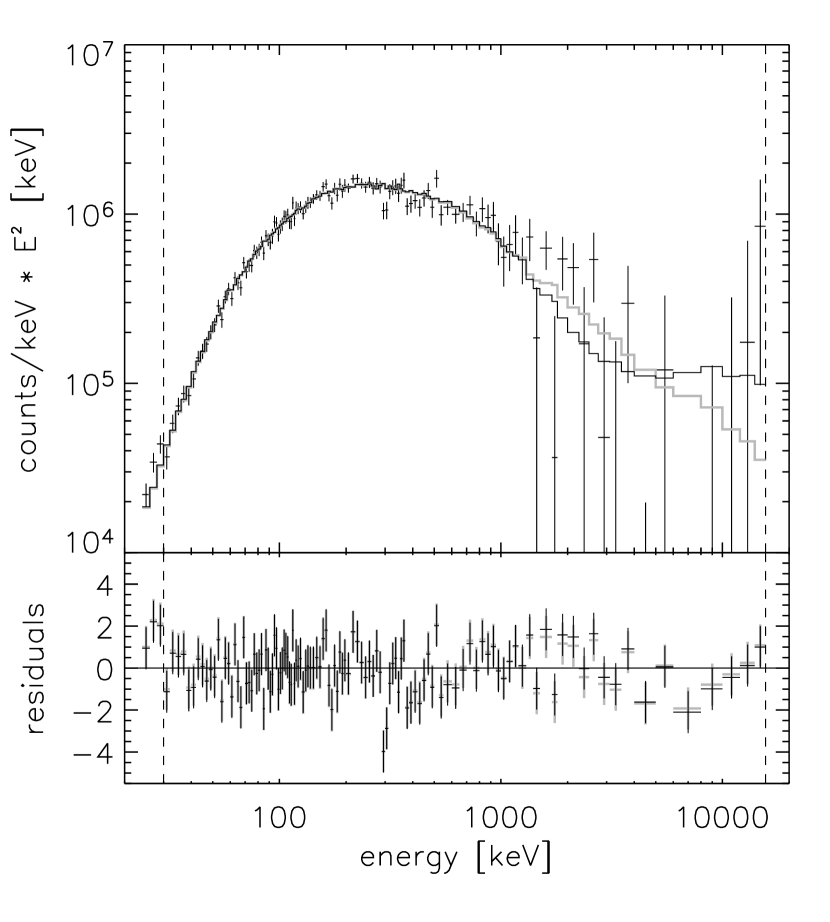
Figure 3: rear spectrum of GRB 020715; error bars: photon counts after background subtraction; black histogram: CBM fit (eq. 10); grey histogram: Band function fit (eq. 7); vertical broken lines: energy range used for fitting; bottom: residuals of CBM (black) and Band (grey) fit.

The measured spectra together with the CBM and Band fits are shown in Figs. 3 to 13. Note that we plot energy${}^{2}\,\cdot\,$counts/keV versus energy. The difference to a deconvolved $E\!\!\cdot\!\!F_{E}$ distribution is discernible e.g. in the drop of counts towards lower energies in our representation. The statistical scatter from the limited number of simulated events is sometimes visible as a little roughness of the simulated spectra.

From the fit parameters obtained for the CBM and the Band function, we calculate the fluences for various energy intervals. They are listed in Table 5. The error of the fluence is dominated by systematics, e.g.  because we do not know the exact active volume of the single detector segments. We estimate the systematic error to be of order 5%, whereas the statistical error is of order 1%. Note also, that the two fluences obtained by fitting CBM and Band function are nearly equal.

4.1 GRB 020715

The lightcurve is shown in Fig. 1 (top) and the spectrum is shown in Fig. 3. Two bins from 290 keV to 310 keV (a background line) and one bin from 500 keV to 525 keV (the 511 keV line) were omitted in the fit because they would dominate $\chi^{2}$. The best fit is a Band function, but the CBM also fits well.

4.2 GRB 021008

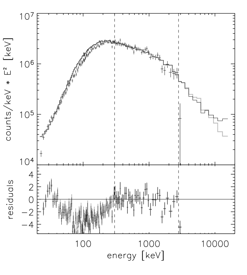
Figure 4: front spectrum of GRB 021008; explanations see caption of Fig. 3; the same set of parameters (eqs. 11 and 12) is used for this plot and Fig. 5.

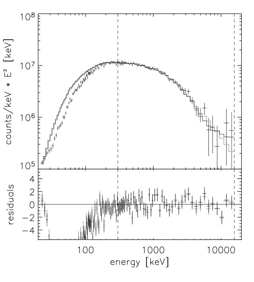
Figure 5: rear spectrum of GRB 021008; explanations see caption of Fig. 3. the same set of parameters (eqs. 11 and 12) is used for this plot and Fig. 4.

Coming from a direction about 50 degrees from the Sun, this GRB deposited photons not only in rear detectors but also in the front detectors, as can be seen from the lightcurve in Fig. 1. The front spectrum is shown in Fig. 4 and the rear in Fig. 5.

Fit

We had difficulties to fit front and rear spectra consistently below 300 keV. We therefore chose 300 keV as the lower energy bound. Band function and CBM give the best fits.

We fitted front and rear segments separately, as well as jointly. The results of the joint fit are shown in Figs. 4 and 5 . For the joint CBM fit we find the 90% confidence level (CL) errors:

$$T_{p} = 641\;^{+54}_{-53}\mbox{ keV}$$

$$\alpha = 1.523\;^{+0.099}_{-0.098}$$ (11)

$$\beta \equiv 2.1$$

$$b = 0.0198\;^{+0.0129}_{-0.0137}$$

The total $\chi^{2}$ is $71.2$ for $n_{DoF}=74$. The Band function fits marginally better, $\chi^{2}=70.0$ for $n_{DoF}=74$ and its parameters are (90% CL errors):

$$E_{p} = 677\;^{+51}_{-66}\mbox{ \mbox{keV}}$$

$$\alpha = 1.493\;^{+0.104}_{-0.104}$$ (12)

$$\beta = 3.73\;^{+0.48}_{-0.38}$$

Discussion

We do not well understand the spectrum below 300 keV. Both fits, the CBM and the Band function, overestimate the counts below 300 keV. This can be a hint that the GRB spectrum hardens below 300 keV. We find functions that fit the front and the rear data from 40 keV to 400 keV individually, but they do not agree.

One possible explanation is the GRB incoming angle of about 50 degrees at which the GRB photons pass through a certain amount of material before reaching the detectors. Our GEANT simulation tries to take that into account, but it is probably not perfect, and maybe the averaging over all rotation angles is a bad assumption for this short GRB pulse.

Another difficulty for this GRB is its background. For the single rear segments, the background at low energies (below $\approx 120$ keV) strongly depends on the rotation angle of RHESSI. We did our best to take this into account, but maybe did not succeed completely.

4.3 GRB 021206

GRB 021206 is famous for its claimed polarization (Coburn & Boggs, 2003), which however turned out to be an artefact (see Rutledge & Fox, 2004; Wigger et al., 2004, 2005). This GRB was also studied by Boggs et al. (2004) to probe quantum gravity.

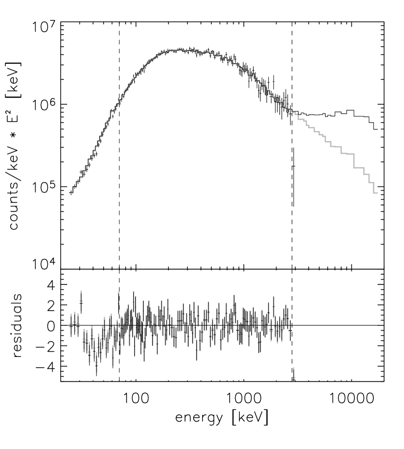
Figure 6: spectrum of GRB 021206, front detectors; explanations see caption of Fig. 3. the same set of parameters (eqs. 13 and 14) is used for this plot and Fig. 7.

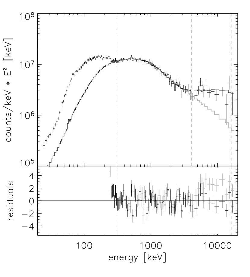
Figure 7: top: spectrum of GRB 021206, rear detectors; symbols as in Fig. 3. bottom: residuals of CBM fit (black) and Band fit (grey). The Band function was fitted only up to 4.5 MeV. The excess counts below 300 keV are backscatters from Earth, see text. The same set of parameters (eqs. 13 and 14) is used for this plot and Fig. 6.

This GRB is only 18 degrees from the Sun, exposing mainly the front segments of RHESSI’s detectors. Its lightcurve is shown in Fig. 1. Fig. 6 shows the energy spectrum in the front segments, Fig. 7 in the rear segments.

Fit

The front spectrum can be fit from 70 keV up to 2800 keV, and the rear from 300 keV to 16 MeV. The huge number of excess counts below $300$ keV in the rear detectors is understood: The geometrical constellation of the GRB, RHESSI, and Earth was such that the GRB photons came from the front direction, where the effective area is relatively small, whereas the Earth was behind RHESSI so that the backscattered photons could easily reach the rear segments.

The only function that fits the front and rear spectra over the entire energy range from 70 keV up to 16 MeV is the CBM. Fitting front and rear spectra simultaneously with CBM and all parameters free, yields (90% CL errors):

$$T_{p} =678\;^{+13}_{-10}\mbox{ \mbox{keV}}$$

$$\alpha =0.60\;^{+0.09}_{-0.08}$$ (13)

$$\beta =2.12\;^{+0.08}_{-0.13}$$

$$b =0.108\;^{+0.039}_{-0.045}$$

with $\chi^{2}=187.5$ for $n_{DoF}=185$. These values are used for the black line histogram and the residuals in Figs. 6 and 7.

The front spectrum alone is well described by a Band function. Its $\chi^{2}$ is even marginally smaller than that of the CBM model fit, see Table 2. The Band function also fits the rear spectrum up to 4.5 MeV with $\chi^{2}=72.8$ (62 DoF), but not at higher energies. The front and rear parameters (up to 4.5 MeV) agree, see Table 4. Evaluating the full parameter space simultaneously for front and rear yields (90% CL errors):

$$E_{p} =711\;^{+15}_{-17}\mbox{ \mbox{keV}}$$

$$\alpha =0.692\;^{+0.033}_{-0.039}$$ (14)

$$\beta =3.19\pm 0.08$$

with $\chi^{2}=176.5$ for $n_{DoF}=174$. These values are used for the grey line histogram in Figs. 6 and 7. They agree with the preliminary results by Wigger et al. (2007). Above 4.5 MeV, a PL with $\gamma=2.23\pm 0.21$ fits the data ($\chi^{2}=12.5$ for 10 DoF).

Discussion

As can be learned from Table 2, the high energy part can not be fit by Band, BPL or CPL, and the low energy part of the spectrum can not be fit by BBPL nor by BBmPL. The only function that fits over the whole RHESSI energy range is CBM.

The CBM function has one parameter more than the Band function. An F-test indicates that the chance probability of producing such an improvement in $\chi^{2}$ with the additional parameter is only $4.0\times 10^{-9}$. The spectral hardening at 4.5 MeV is significant.

Because this GRB has so many counts at high energies, we used a simulation with $\gamma_{sim}=1.75$ for the results cited above. A power law index of 1.75 results in relatively more counts at high energies than the usual power law index (=2). We also used simulations with $\gamma_{sim}=1.5$ and $\gamma_{sim}=2.0$. The results were almost identical, especially for the high energy parameters $\beta$ and $b$ of the CBM fit.

The high energy photon index $\beta$ of the CBM function agrees perfectly with the theoretical expected value ($\approx 2.1$). The low energy photon index $\alpha\approx 0.6$ on the other hand is slightly smaller than expected from theory ($\approx 1.0$).

Peak resolved analysis

The time structure of GRB 021206 is rather intricate. Four periods of emission can be distinguished, see Fig. 1, each of them probably consisting of several overlaying sub-peaks. Luckily, these time periods match quite well our minimum time resolution of one third of a rotation period for fitting with a rotation averaged response function (see §2.3).

The fitted parameters are listed in Table 6 for the four time intervals marked in the figure, as well as the additional tail interval. The tail interval lasts one full rotation, starting at the end of the P4 interval. The fluences of the two components in the CBM function (eq. 10) are listed separately ($F_{\mbox{\scriptsize CPL}}$ for the CPL component and $F_{\mbox{\scriptsize mPL}}$ for the modified PL component). The mPL index $\beta$ was kept frozen at 2.1.

The energy $T_{p}$ increases from the first to the second time interval and then decreases. Also $F_{CPL}$ and $F_{mPL}$ increase from the first to the second interval, and then decrease. However, the modified PL component seems to decay more slowly than the CPL component. The tail is dominated by the mPL component.

4.4 GRB 030329

GRB 030329 is famous for the supernova 2003dh detected in its afterglow (Hjorth et al., 2003; Matheson et al., 2003; Chornock et al., 2003; Zaritsky et al., 2003). The authors of the CBM model used the lightcurve of this GRB and its early afterglow to predict the later afterglow and the appearance of a supernova (see Dado, Dar & de Rújula, 2003b). A supernova and the late afterglow was also predicted by Zeh et al. (2003), and is discussed in Ferrero et al. (2006).

In the lightcurve of GRB 030329, two peaks are clearly separated (Fig. 1, bottom plot). We analyse them separately.

Fit

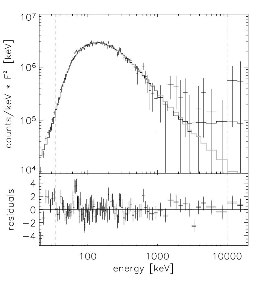
Figure 8: rear spectrum of GRB 030329, first peak; explanations see caption of Fig. 3.

The spectrum of the first peak is shown in Fig. 8. Three bins around a background line from 64 keV to 70 keV were not included in the fit. A very good fit (see Table 2) is a CPL with: $E_{\mbox{\em\scriptsize peak}}=158.7\pm 5.0\mbox{ keV}$ and $\alpha=1.662\pm 0.032.$ Not surprisingly, the CBM and Band function, having more parameters, but being closely related to a CPL, fit only marginally better.

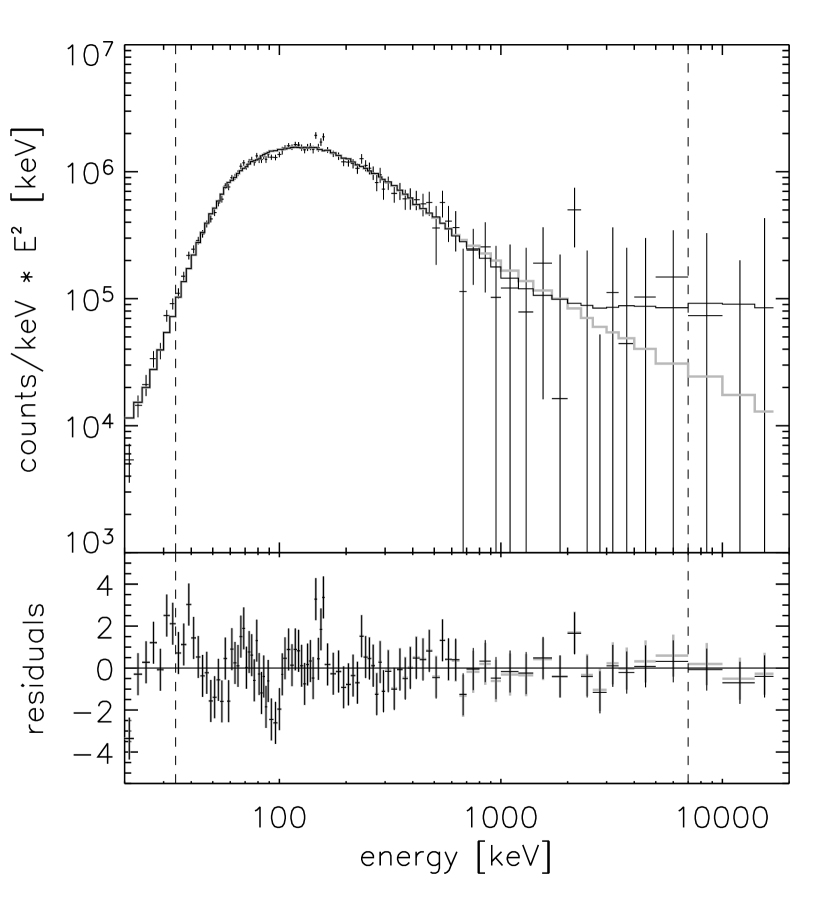
Figure 9: rear spectrum of GRB 030329, second peak; explanations see caption of Fig. 3.

The spectrum of the second peak is shown in Fig. 9. The spectrum has some wiggles below 160 keV, which account for the relatively high $\chi^{2}$. Many models give an acceptable fit, only BBPL does not fit. A good fit (see Table 2) is a CPL with $E_{\mbox{\em\scriptsize peak}}=78\pm 13\mbox{ keV}$ and $\alpha=1.83\pm 0.05$. Also a good fit is a broken power law (BPL) with $E_{b}=175\pm 15\mbox{ keV}$, $\alpha=1.985\pm 0.032$, and $\beta=2.68\pm 0.08$. Also Band function and CBM model fit the data well, see Fig. 9.

Discussion

The prompt emission was detected by HETE. Its spectrum is published by Vanderspek et al. (2004) and by Sakamoto et al. (2005). Vanderspek et al. (2004) do a time resolved analysis. For the entire burst they find (90% CL errors): $E_{\mbox{\em\scriptsize peak}}=70.2\pm 2.3$ keV, $\alpha=1.32\pm 0.02$, $\beta=2.44\pm 0.08$. Sakamoto et al. (2005) find for the entire burst (90% CL errors): $E_{\mbox{\em\scriptsize peak}}=68\pm 2$ keV, $\alpha=1.26\pm 0.02$, $\beta=2.28\pm 0.06$.

The RHESSI parameters, for both peaks, are all significantly higher (see Table 4). However, the high energy photon indices can not be compared directly, because the break energy (above which $\beta$ is determined, see eq. 7) for HETE is 116 keV, whereas for RHESSI it is $>400$ keV, i.e. above the HETE energy range. Fitting the RHESSI data (for the entire duration of the burst) from 135 keV to 500 keV only, where the RHESSI response is good, we find $\beta=2.441\pm 0.032$, in excellent agreement with HETE. Fitting the RHESSI data from 400 keV to 2000 keV, i.e. above the HETE range, we find $\beta=3.11\pm 0.25$. The spectrum seems to soften above $\approx 350$ keV.

The high RHESSI value for $\alpha$ (almost 2.0) for the second lightcurve peak indicates that the spectral peak (in the $E\!\!\cdot\!\!F_{E}$ representation) is broad. Since RHESSI’s sensitivity drops below $\approx 80$ keV, and this is a GRB with $E_{\mbox{\em\scriptsize peak}}$ in the order of 100 keV, it is likely that RHESSI’s $\alpha$ describes rather the broadness of the peak than the low energy photon index. This opinion is supported by the fit result of the BPL fit. The low energy photon index $\alpha\approx 2.0$ shows that the $E\!\!\cdot\!\!F_{E}$ spectrum is flat from 34 keV to 175 keV.

It should also be mentioned that the $\chi^{2}$ of the HETE fit, as cited by Sakamoto et al. (2005), is very bad. Also the RHESSI $\chi^{2}$ of the spectral fits for the second peak are rather high. A joint fit of RHESSI and HETE data might reveal interesting features.

4.5 GRB 030406

Fit

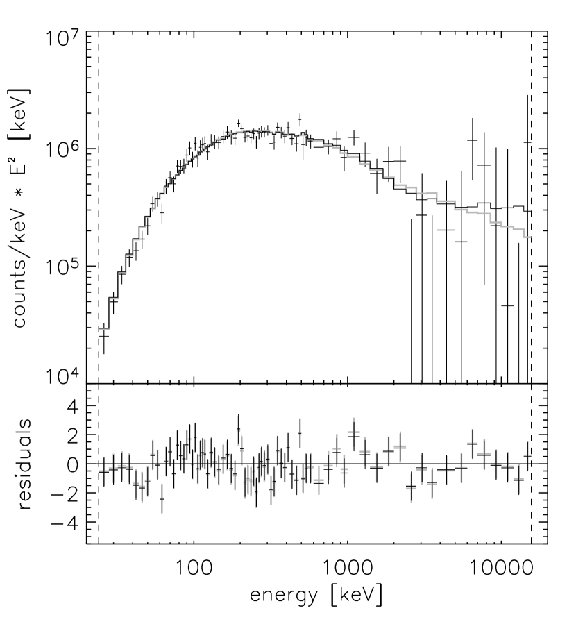
Figure 10: rear spectrum of GRB 030406; explanations see caption of Fig. 3.

The lightcurve is shown in Fig. 2 (top) and the spectrum is shown in Fig. 10. The best fit is the CBM function with the parameters $\alpha$ and $\beta$ frozen at the theoretical values. The next best fit is the Band function.

discussion

The spectrum of this burst was also studied by Marcinkowski et al. (2006) using data from the INTEGRAL satellite. For the spectral analysis, they used combined ISGRI and IBIS Compton mode data. The time interval used by Marcinkowski et al. (2006) differs from ours. Using a similar time interval as their ‘peak’ time interval, we find:

$\bullet$ Fit of a BPL from 24–2400 keV (comparable to the energy range in the analysis by Marcinkowski et al. (2006)): fits well ($\chi^{2}=70.3$ for $n_{DoF}=60$), and the parameters are: $E_{b}=479\pm 80$ keV, $\alpha=1.08\pm 0.05$, $\beta=1.96\pm 0.02$.

$\bullet$ Fit of a BPL from 24 keV to 16 MeV: does not fit well ($\chi^{2}=86.0$ for $n_{DoF}=71$).

$\bullet$ Fit of CBM from 24 keV to 16 MeV with $\alpha=1.0$ and $\beta=2.1$ frozen: fits well ($\chi^{2}=77.9$ for $n_{DoF}=72$), and the parameters are: $T=1220\pm 110$ keV and $b=0.055\pm 0.079$,

$\bullet$ Fit of Band function: fits well ($\chi^{2}=77.33$ for $n_{DoF}=71$), and the parameters are: $E_{\mbox{\em\scriptsize peak}}=1180\pm 120$ keV, $\alpha=0.96\pm 0.06$, $\beta=3.02\pm 0.55$.

For the high energy part, the parameters found by Marcinkowski et al. (2006) and by us agree. But we can not confirm their hard low energy photon index $\alpha<0.0$. We even dare to say that we trust our low energy photon index better, because for this GRB incoming direction, the RHESSI response function is well understood, whereas the INTEGRAL response function of this burst might suffer from same systematic effects that we described for RHESSI in §2.4.

4.6 GRB 030519B

Fit

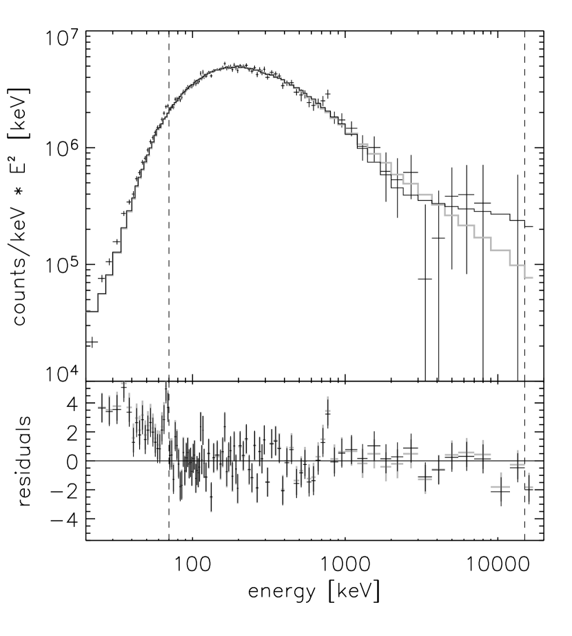
Figure 11: rear spectrum of GRB 030519B; explanations see caption of Fig. 3.

The lightcurve is shown in Fig. 2 and the spectrum in Fig. 11. The best fit is the Band function, followed by CBM.

Discussion

In the HETE GRB catalog by Sakamoto et al. (2005) one finds (90% CL errors): $E_{p}=138\;^{+18}_{-15}$ keV, $\alpha=0.8\pm 0.1$, $\beta=1.7\pm 0.2$. Since $\beta<2.0$, the energy $E_{p}$ is not the peak energy, but only a variable related to the parameter $E_{0}=E_{p}/(2-\alpha)$. Indeed, the RHESSI peak energy for this GRB is $>400$ keV. But the HETE parameters do not fit the RHESSI spectrum from 70 keV to 350 keV ($\chi^{2}=141$ for 53 energy bins).

4.7 GRB 031027

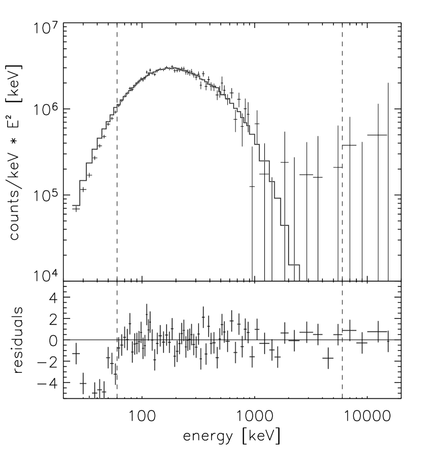
Figure 12: rear spectrum of GRB 031027; histogram and residuals: fit of a cut off power law (CPL); a CPL is equivalent to a Band function with $\beta=\infty$ or CBM with $b=0$.

The lightcurve is shown in Fig. 2 and the spectrum in Fig. 12. The best fit is a cut off power law with $E_{\mbox{\em\scriptsize peak}}=336\pm 9$ keV and $\alpha=0.940\pm 0.05$. This function is shown in Fig.  12. Band function and CBM have difficulties to converge. Since the CPL fits so well, we expect $\beta=\infty$ for the Band function and $b=0$ for the CBM function.

4.8 GRB 031111

Fit

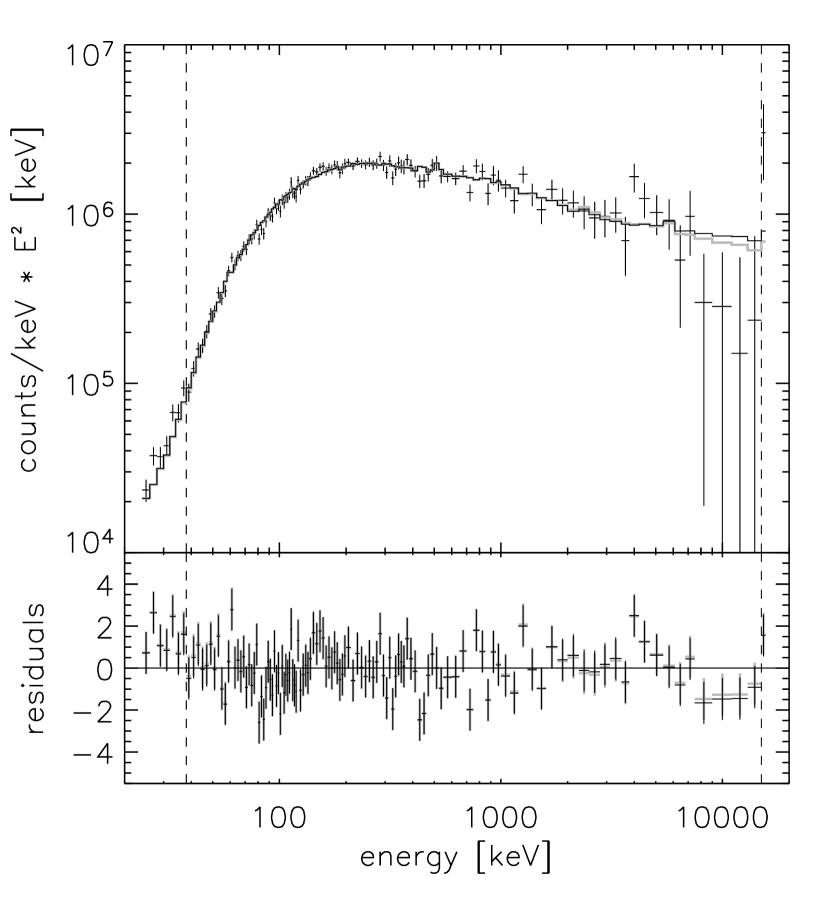
Figure 13: rear spectrum of GRB 031111; explanations see caption of Fig. 3.

The lightcurve is shown in Fig. 2 (bottom) and the spectrum is shown in Fig. 13. Band function, CBM and BBmPL are good fits, the best being Band function.

Discussion

A preliminary CPL fit to the HETE data is published on a web page as $E_{0}=600.5$ keV and $\alpha=0.8366$ with a good $\chi^{2}$. These values describe the RHESSI spectrum well from 80 keV to 350 keV, but not at higher energies. HETE’s energy range ends at 400 keV, thus we believe that our values for $E_{0}$ and $\alpha$ are better.

5 GENERAL DISCUSSION AND CONCLUSION

5.1 The spectral functions

What is an acceptable $\chi^{2}$? In the limit of many degrees of freedom ($n_{DoF}>30$), $\chi^{2}$ is normal distributed with an expectation value of $n_{DoF}-0.5$ and a variance of $\sigma_{\chi^{2}}=\sqrt{2n_{DoF}-1}$. A fit is acceptable if $\chi^{2}$ is close to its expectation value and if the residuals scatter around zero over the whole fit range, i.e. if the fit “looks good”.

From Table 2 we conclude that the CBM gives acceptable $\chi^{2}$ for all GRBs studied. And they also look good, as can be seen in Figs. 3 to 13. Except for GRB 021206, rear (Fig. 7), the same can be said for the Band function.

In many cases, a cut off power law (CPL) fits the spectrum up to high energies, e.g. GRB 021008, GRB 030329 or GRB 031027. In these cases, Band and CBM improve the goodness-of-fit slightly, but all three spectral shapes fit the data acceptably.

A broken power law fits sometimes, but usually not well.

BBPL and BBmPL do not fit in general, BBPL worse than BBmPL. However, it should be mentioned that a blackbody component is expected—if at all—only at the beginning of a GRB (see e.g. Ryde et al. (2006) and references therein), whereas we fitted the entire duration of the bursts. When using BBPL, we often find that the PL component fits either at high energies or at low energies. This is also discussed by Ghirlanda et al. (2007) who studied six BATSE GRBs in detail, where low energy data from the WFC instrument (on board BeppoSAX) are available. They find that the WFC data fit the Band function or CPL extrapolation, but not the BBPL extrapolation to low energies. Arguing that the PL contribution is too simple, they try to fit a blackbody spectrum plus CPL. We suggest to use our BBmPL function instead. Its modified PL component describes a spectral break from $dN/dE\propto E^{-(\beta-1)}$ at low energies to $dN/dE\propto E^{-\beta}$ at high energies.

5.2 CBM function

The present work is, to our knowledge, the first systematic attempt to fit the CBM function to prompt GRB spectra. The two terms in eq. 10 have a simple meaning. According to the cannonball theory, all GRBs are associated with a supernova. The ambient light is Compton up-scattered by the cannonball’s electrons, producing the prompt GRB emission. Some electrons are simply comoving with the cannonball, giving rise to the CPL term in eq. 10. Since the photon spectrum of the ambient light can be described by a thin thermal bremsstrahlung spectrum, $\alpha$ is expected to be $\approx 1$. The second term (mPL) is caused by a small fraction of electrons accelerated to a power law distribution, resulting in a photon index of $\beta\approx 2.1$. See e.g. Dado & Dar (2005), §3.8. or Dado, Dar & de Rújula (2007), §2 and 4.1 for a summary.

In our study, the observed values for $\alpha$ are all approximately 1, as predicted by the CBM. Because of the low count statistics at high energies, we could not always fit $\beta$. We then fixed it to its theoretical value of 2.1 in order to make the fit converge and to obtain a value for the parameter $b$. In the cases where we could fit $\beta$, we found values close to 2.1 (Table 3).

For the factor $b$ of the modified PL component in the CBM function we typically found values of the order $0.1\,$. An exception is GRB 031111, where $b$ is of the order 1.0, but with a large error ($0.4$).

Our values for $\beta$ and $b$ are similar to the ones found by Dado & Dar (2005) (fit of GRB 941017) and by Dado, Dar & de Rújula (2004) (fit of $X$-ray flashes XRF 971019, XRF 980128, and XRF 990520 using BeppoSAX/WFC and CGRO/BATSE data). The authors of the CBM hypothesize that XRFs are simply GRBs viewed further off the jet axis.

The different time development of the CPL- and the mPL-fluences, as reported in Table 6, possibly point to a different time dependence of the two underlying electron distributions within a cannonball.

5.3 Fitting CBM function versus CPL and Band function

Both the Band function and the CBM function are extensions of a CPL, the Band function with one additional parameter, the CBM function with two. For cases where a CPL fits the data well, also a Band function with $\beta=\infty$ or a CBM function with $b=0$ (and $\beta=2.1$ or any other value) fits. This is the case for GRB 031027.

Whether additional parameters are necessary in a fit, can be tested with the $F$-test. For GRB 030329, the extra parameters are barely needed. For GRB 020715, 021008, 021206, 030406, 030519B, 031111 additional parameters are required at a confidence level of at least 90%.

Concerning the question of whether the high energy power law parameter $\beta$ in the CBM should be treated as free parameter, the answer is ’yes’ from a theoretical point of view, but in practice, see Table 2, the improvements in $\chi^{2}$ are marginal or small for all bursts we studied. Our practice to freeze $\beta$ at its theoretically predicted value in cases of bad convergence seems to be acceptable.

It is more difficult to compare the goodness of fit using the Band function compared to using the CBM function. The two functions are not independent, because they both are dominated by a CPL up to the peak energy and higher. In most cases of our study, the two functions fit the observed spectrum equally well with a slight preference for the Band function. At high energies however (typically above several times the peak energy) the two functions are different, the spectral hardening being a unique feature of the CBM function. There is only one case, namely GRB 021206, where this hardening is observed. For the rear data going up to high energies, a Band function fit gives $\chi^{2}/\mbox{dof}=133.3/74$ (see Table 2). This is not acceptable at $<0.01$% probability of being accidentally so high. The CBM fit on the other hand gives $\chi^{2}/\mbox{dof}=82.7/73$, which is fully acceptable at a $20$% level.

We would like to stress again that, while the CBM gives acceptable fits for all cases, the Band function fails in one case. This seems enough to us to give some credit to the CBM.

But it is, of course, no proof that the CBM is the only theory capable of describing the spectrum of GRB 021206. For example, a Band function plus a PL with $\gamma\approx 1.5$ would also fit. But there is no theory to predict such a shape. To our knowledge, CBM is to date the only existing GRB model that explains the prompt GRB spectra from first principles.

At this place we also would like to note the the mean $\alpha$-value found for the BATSE catalogue is 1 (see Kaneko et al., 2006)). We cite from their summary: “We confirmed, using a much larger sample, that the most common value for the low-energy index is $\approx-1\,$ (Preece et al., 2000; Ghirlanda et al., 2002). The overall distribution of this parameter shows no clustering or distinct features at the values expected from various emission models, such as $-2/3$ for synchrotron (Katz et al., 1994; Tavani, 1996), $0$ for jitter radiation (Medvedev, 2000), or $-3/2$ for cooling synchrotron (Ghisellini & Celotti, 1999).” They do not mention the CBM which would explain $\alpha\approx 1$.

Note that the $\beta$ values of the CBM are systematically lower than the $\beta$ values of the Band function, compare Tables 3 and 4. From Band function fits to BATSE GRBs, it is known that $\beta$ is clustered around 2.3, with a long tail towards higher values, see Kaneko et al. (2006). For CBM we would expect $\beta$ to cluster at slightly lower values.

For criticism of the CBM, see e.g. Hillas (2006), but see also the answer by Dar & de Rújula (2006).

5.4 The spectral hardening

The difference of a CBM spectrum and Band function is the hardening at high energies. This becomes visible—for the GRBs studied here—in the few MeV region, but it depends on the peak energy and the factor $b$. For $\alpha=1.0$ and $b=0.10$ the hardening typically appears at several times the peak energy and the second term dominates at 10 times the peak energy. For the spectral fit of XRFs done by Dado, Dar & de Rújula (2004), the spectral hardening is expected in the few hundred keV region, just where the number of photons detected runs low. Most of our GRBs also suffer from this lack of statistics at high energies, preventing the detection of a hardening.

A spectral coverage of two decades and good detection efficiency at high energies is necessary to experimentally observe the full shape of the CBM function. In the case of GRB 021206 we were able to detect this hardening, thanks to RHESSI’s broad energy range (30 keV to 15 MeV), and because this is one of the brightest GRBs ever observed.

There is a GRB observed by SMM from 20 keV up to 100 MeV, namely GRB 840805. As reported by Share et al. (1986), the spectrum of this burst shows emission up 100 MeV. In order to fit the spectrum, “a classical thermal synchrotron function plus a power law” was used. The power law component was required to fit the data above about 6 MeV. This is a hint of a spectral hardening around 6 MeV, and we suppose that the spectrum of this GRB can be fit by a CBM function.

The spectral hardening observed in GRB 941017 (González et al., 2003) seems to be different. The photon index of GRB 941017 above a few MeV is $\approx 1.0$. This case is discussed by Dado & Dar (2005) as a possible additional feature in the CBM spectrum.

5.5 Outlook

In order to find more GRB spectra that show the hardening characteristic for the CBM function, strong GRBs have to be observed over a broad enough energy range. With the forthcoming GLAST mission, we expect that more such spectra will be observed. But also joint analyses with more than one instrument could reveal this hardening. We therefore suggest:

$\bullet$ to search for CBM spectrum candidates among joint Swift/RHESSI GRBs and XRFs, and joint Swift/Konus GRBs.

$\bullet$ to reanalyse some BATSE bursts. Looking at the BATSE spectra published by Ghirlanda et al. (2007), we suppose that the CBM can possibly improve the fits of GRB 980329, GRB 990123, and GRB 990510. The same can be said for GRB 911031 as published by Ryde et al. (2006). And GRB 000429, as published in Fig. 19 of Kaneko et al. (2006), looks like a promising candidate as well.

$\bullet$ to search in KONUS data for suitable GRBs.

$\bullet$ to add the CBM function to XSPEC in order to make it more accessible to the astronomical community.

6 SUMMARY

We have presented the time integrated spectra of 8 bright GRBs observed by RHESSI in the years 2002 and 2003.

The spectrum of GRB 021206 shows a hardening above 4 MeV. From 70 keV to 4.5 MeV, the spectrum can be well fitted by a Band function – but not above that. The cannonball model successfully describes the entire spectrum up to 16 MeV, the upper limit of RHESSI’s energy range. For the spectra of the seven other GRBs analysed, we found that they can be fitted by the CBM as well as by the Band function.

We therefore suggest that the cannonball model should be considered for fitting GRB spectra.

Table 1: GRB analysis time intervals

GRB	$t_{0}$	$\Delta t_{burst}$	$\Delta t_{BG1}$	$\Delta t_{BG2}$	$\theta$	ref.
	(UT)	(s)	(s)	(s)	(degrees)
020715	19:20:56.0	[11.53,15.55]	[0-80.46,0.0]	[048.28,168.97]	072.4	1
021008	07:00:45.0	[17.21,21.29]	[0-73.37,0.0]	[036.68,048.91]	050.1	2
021206	22:49:11.7	[02.73,08.19]	[0-53.26,0.0]	[020.49,102.43]	018.0	3
030329 P1	11:37:10.0	[16.56,24.84]	[0-70.39,0.0]	[070.39,140.78]	144.1	4
030329 P2	”	[28.98,34.50]	”	”	”	”
030406	22:41:30.0	[85.68,89.83]	[-140.96,0.0]	[140.96,281.93]	096.1	5
030519B	14:04:53.0	[00.46,11.47]	[0-61.94,0.0]	[028.90,090.84]	165.5	6
031027	17:07:06.0	[29.71,45.92]	[-137.77,0.0]	[068.88,206.65]	101.5	7
031111	16:45:12.0	[02.27,06.35]	[-122.51,0.0]	[012.25,134.76]	155.6	8

Note. — $t_{0}$: reference time; $\Delta t_{burst}$: time interval for spectral analysis; $\Delta t_{BG1}$: background time interval before GRB; $\Delta t_{BG2}$: background time interval after GRB; time intervals are given relative to $t_{0}$. $\theta$: angle between GRB direction and RHESSI axis; References: (1) GCN 1456, 1454 (Hurley et al., 2002a), (2) GCN 1629, 1617 (Hurley et al., 2002b), (3) GCN 1728, 1727 (Hurley et al., 2002c), (4) GCN 1997 (Vanderspek et al., 2003), (5) GCN 2127 (Hurley et al., 2003a), (6) GCN 2235, 2237 (Lamb et al., 2003; Hurley et al., 2003c), (7) GCN 2438 (Hurley et al., 2003d), (8) HETE trigger 2924, GCN 2443 (Hurley et al., 2003e).

Table 2: Chi-square of spectral fits

GRB	$\Delta E_{\mbox{\scriptsize front}}\,$	$\Delta E_{\mbox{\scriptsize rear}}\,$	$n$	CPL	Band	CBM	CBM	BPL	BBPL	BBmPL
	(keV)	(keV)		$n_{par}=3$	4	4	5	4	4	4
020715	$\cdots$	[030,15660]	117	113.9	106.3	110.8	110.7	129.2	270.0	157.1
021008	[300,2800]	$\cdots$	38	35.5	34.8	35.1	35.0	33.0	32.9	33.9
021008	$\cdots$	[300,15660]	50	43.8	39.2	39.9	39.2	52.9	97.4	60.2
021008	[300,2800]	[300,15660]	88	$\cdots$	79.5	80.8	$\cdots$	$\cdots$	$\cdots$	$\cdots$
021206	[070,2800]	$\cdots$	112	130.6	103.6	104.1	103.9	155.5	315.7	191.8
021206	$\cdots$	[300,16000]	78	338.1	133.3	82.7	82.7	132.9	94.1	110.5
021206	[070,2800]	[300,16000]	190	$\cdots$	$\cdots$	$\cdots$	187.5	$\cdots$	$\cdots$	$\cdots$
021206	$\cdots$	[300,04500]	66	$\cdots$	72.8	69.8	$\cdots$	$\cdots$	$\cdots$	$\cdots$
021206	[070,2800]	[300,04500]	178	$\cdots$	176.5	$\cdots$	$\cdots$	$\cdots$	$\cdots$	$\cdots$
030329 P1	$\cdots$	[034,10000]	94	86.5	84.3	84.8	84.7	89.3	137.8	89.1
030329 P2	$\cdots$	[034,07000]	87	104.5	103.3	103.2	103.1	98.9	102.0	98.4
030406	$\cdots$	[024,15000]	75	79.1	75.6	75.0	75.0	88.6	151.2	88.7
030519B	$\cdots$	[070,15000]	79	102.2	86.3	91.1	89.0	99.8	189.8	109.8
031027	$\cdots$	[060,06000]	63	63.6	0n.c.	0n.c.	0n.c.	93.0	138.9	99.6
031111	$\cdots$	[038,15000]	117	182.4	128.3	133.2	130.4	140.5	266.0	133.0

Note. — $\chi^{2}$ obtained by fitting different spectral models to the data. $\Delta E_{\mbox{\scriptsize front/rear}}$: energy interval used to fit front/rear detector data; $n$: number of energy bins; $n_{par}$: number of free fit parameters; CPL: cut off power law eq. 5, Band: Band function eq. 7, CBM: cannonball model eq. 10, BPL: broken power law eq. 6, BBPL: blackbody plus power law eq. 8, BBmPL: blackbody plus modified power law eq. 9; n.c.: fit did not converge. In the case of CBM with 4 parameters, $\beta$ was fixed to its theoretically expected value of $2.1\,$. For each fit, the degree of freedom is $n_{DoF}=n-n_{par}$.

Table 3: Fit results for CBM

GRB	$\Delta E_{\mbox{\scriptsize front}}\,$	$\Delta E_{\mbox{\scriptsize rear}}\,$	$T_{p}\,$	$\alpha$	$\beta$	$b$
	(keV)	(keV)	(keV)
020715	$\cdots$	[030,15660]	532$\pm$20	$0.741\pm 0.077$	2.20$\pm$0.14	string0.067$\pm$0.040
021008	[300,2800]	$\cdots$	628$\pm$71	$1.31\pm 0.28$	2.1	string0.052$\pm$0.076
021008	$\cdots$	[300,15660]	672$\pm$68	$1.487\pm 0.062$	2.77$\pm$0.55	string0.085$\pm$0.092
021008	[300,2800]	[300,15660]	641$\pm$32	$1.523\pm 0.055$	2.1	string0.020$\pm$0.008
021206	[070,2800]	$\cdots$	672$\pm$20	$0.66\pm 0.21$	1.92$\pm$0.67	string0.063$\pm$0.142
021206	$\cdots$	[300,16000]	672$\pm$24	$0.67\pm 0.19$	2.12$\pm$0.13	string0.102$\pm$0.048
021206	[070,2800]	[300,16000]	678$\pm$06	$0.60\pm 0.06$	2.10$\pm$0.08	string0.103$\pm$0.028
021206	$\cdots$	[300,04500]	670$\pm$23	$0.71\pm 0.15$	2.1	string0.091$\pm$0.012
021206	[070,2800]	[300,04500]	$\cdots$	$\cdots$	$\cdots$	$\cdots$
030329 P1	$\cdots$	[034,10000]	147$\pm$10	$1.614\pm 0.036$	2.1	string0.033$\pm$0.029
030329 P2	$\cdots$	[034,07000]	069$\pm$15	$1.841\pm 0.049$	2.1	string0.048$\pm$0.055
030406	$\cdots$	[024,15000]	626$\pm$83	$0.966\pm 0.089$	2.1	string0.180$\pm$0.120
030519B	$\cdots$	[070,15000]	396$\pm$12	$0.949\pm 0.073$	2.388$\pm$0.097	string0.135$\pm$0.048
031027	$\cdots$	[060,06000]	340$\pm$17	$0.950\pm 0.055$	2.1	-0.010$\pm$0.025
031111	$\cdots$	[038,15000]	690$\pm$45	$0.68\pm 0.27$	2.241$\pm$0.023	string1.090$\pm$0.360

Note. — $\Delta E_{\mbox{\scriptsize front/rear}}$: energy interval used to fit front/rear detector data; $T_{p},\alpha,\beta,b$: parameters as defined in the text below eq. 10; errors are symmetric $1\sigma$ errors; where no error is given, the parameter was frozen at that value.

Table 4: Fit results for Band function

GRB	$\Delta E_{\mbox{\scriptsize front}}$	$\Delta E_{\mbox{\scriptsize rear}}$	$E_{p}\,$	$\alpha$	$\beta$
	(keV)	(keV)	(keV)
020715	$\cdots$	[030,15660]	$531\pm 24$	$0.776\pm 0.044$	$3.14\pm 0.25$
021008	[300,2800]	$\cdots$	$670\pm 58$	$1.36\pm 0.23$	$3.41\pm 0.51$
021008	$\cdots$	[300,15660]	$678\pm 42$	$1.526\pm 0.067$	$3.86\pm 0.25$
021008	[300,2800]	[300,15660]	$677\pm 33$	$1.493\pm 0.056$	$3.73\pm 0.18$
021206	[070,2800]	$\cdots$	$713\pm 17$	$0.694\pm 0.031$	$3.20\pm 0.13$
021206	$\cdots$	[300,16000]	$\cdots$	$\cdots$	$\cdots$
021206	[070,2800]	[300,16000]	$\cdots$	$\cdots$	$\cdots$
021206	$\cdots$	[300,04500]	$709\pm 18$	$0.72\pm 0.20$	$3.186\pm 0.063$
021206	[070,2800]	[300,04500]	$711\pm 7\phantom{0}$	$0.692\pm 0.020$	$3.19\pm 0.04$
030329 P1	$\cdots$	[034,10000]	$157.2\pm 5.2$	$1.608\pm 0.038$	$3.48\pm 0.53$
030329 P2	$\cdots$	[034,07000]	$\phantom{0}85\pm 11$	$1.781\pm 0.065$	$3.04\pm 0.30$
030406	$\cdots$	[024,15000]	$674\pm 70$	$0.979\pm 0.064$	$2.61\pm 0.27$
030519B	$\cdots$	[070,15000]	$417\pm 13$	$1.048\pm 0.042$	$3.11\pm 0.18$
031027	$\cdots$	[060,06000]	$338\pm 15$	$0.940\pm 0.079$	$\cdots$
031111	$\cdots$	[038,15000]	$844\pm 59$	$1.102\pm 0.036$	$2.364\pm 0.068$

Note. — $\Delta E_{\mbox{\scriptsize front/rear}}$: energy interval used to fit front/rear detector data; $E_{p},\alpha,\beta$: parameters as defined in the text below eq. 7; where no $\beta$ is given, a CPL (eq. 5) was fitted; errors are symmetric $1\sigma$ errors.

Table 5: Fluences in $10^{-5}\,$erg cm^-2

GRB	$F_{\mbox{\scriptsize CB}}$	$F_{\mbox{\scriptsize Band}}$	$F_{\mbox{\scriptsize RHESSI}}$	$F_{\mbox{\scriptsize HETE}}$	HETE	$F_{\mbox{\scriptsize Ulysses}}$	Ulysses
	($10^{-5}\,$erg cm-2)
020715	4.37	4.41	3.94	1.93	$\cdots$	0.43	0.30
021008 front	26.85	26.85	41.24	22.92	$\cdots$	8.67	$\cdots$
021008 rear	35.54	35.64	48.85	27.15	$\cdots$	10.27	8.5
021206 front	52.15	52.44	55.67	19.97	$\cdots$	3.81	$\cdots$
021206 rear	58.74	53.45	70.55	25.29	$\cdots$	4.82	16
030329 P1	6.51	6.47	4.42	5.20	$\cdots$	2.57	$\cdots$
030329 P2	3.58	3.58	2.26	2.95	$\cdots$	1.69	$\cdots$
030329 total	$\cdots$	$\cdots$	7.35	9.46	$10.76\pm 0.14$	4.93	$\cdots$
030406	4.81	4.81	4.26	1.62	$\cdots$	0.40	1.3
030519B	10.27	10.36	9.56	6.07	$6.10\pm 0.1$	1.78	$\cdots$
031027	5.37	5.45	4.81	3.97	$\cdots$	1.17	1.4
031111	7.40	7.40	6.59	2.10	1.714	0.56	0.21

Note. — $F_{\mbox{\scriptsize CB}}$: fluence from CBM fit (Table 3); $F_{\mbox{\scriptsize Band}}$: fluence from Band function fit (Table 4); $F_{\mbox{\scriptsize RHESSI}}$: fluence in [100,10000] keV (RHESSI range); $F_{\mbox{\scriptsize HETE}}$: fluence in [30,400] keV (HETE range); $F_{\mbox{\scriptsize Ulysses}}$: fluence in [25,100] keV (Ulysses range); HETE: HETE fluences from references cited in §4; Ulysses: Ulysses fluences from references cited in Table 1.

Table 6: Peak resolved analysis of GRB 021206

$\Delta t$	duration	$T_{p}$	$\alpha$	$\beta$	$b$	$F_{CPL}$	$F_{mPL}$
	(s)	(keV)				($10^{-5}\,$erg cm-2)
P1	1.366	$661\pm 18$	$0.77\pm 0.06$	$2.1$	$0.059\pm 0.010$	11.7	03.0
P2	1.366	$732\pm 12$	$0.42\pm 0.05$	$2.1$	$0.115\pm 0.010$	14.5	12.9
P3	1.366	$684\pm 14$	$0.63\pm 0.05$	$2.1$	$0.085\pm 0.012$	12.7	06.3
P4	1.366	$530\pm 20$	$0.80\pm 0.08$	$2.1$	$0.113\pm 0.018$	06.9	03.8
tail	4.097	$160\pm 60$	1.0	$2.1$	$2.5\;^{+\infty}_{-1.5}$	00.2	03.1

Note. — $\Delta t$: time period, cf. Fig. 1; $T_{p}$, $\alpha$, $\beta$ and $b$: CBM parameters; $F_{\mbox{\scriptsize CPL}}$: fluence of the CPL-component in the CBM function (eq. 10), $F_{\mbox{\scriptsize mPL}}$: fluence of the modified PL component of eq. 10; fluences are for the range [100,10000] keV.

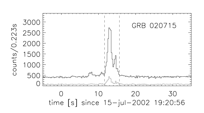
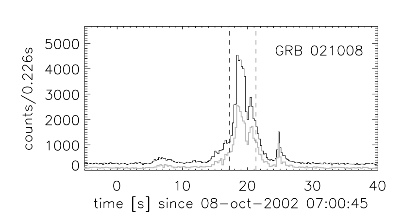
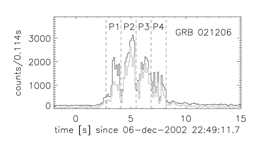
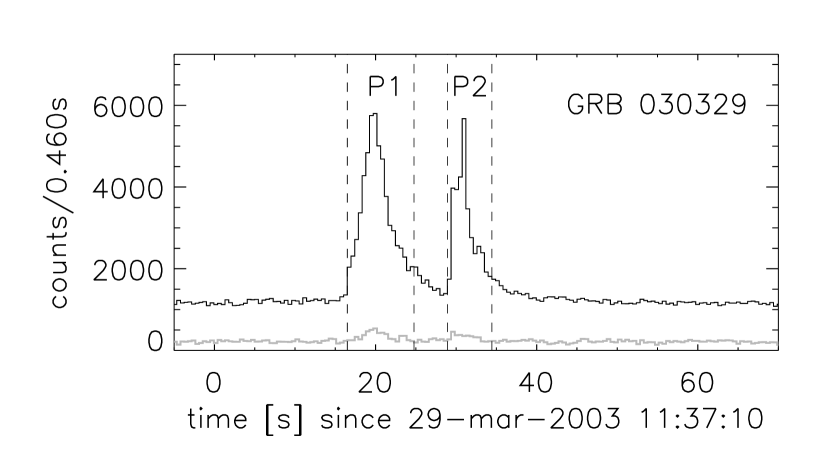
Figure 1: lightcurves for the energy band 20 keV to 3 MeV; black: rear detectors, grey: front detectors; broken vertical lines: time intervals used for spectral analysis.

References

- Band et al. (1993) Band, D. et al. 1993, ApJ 413, p. 281.
- Barlow & Beeston (1993) Barlow, R. & Beeston, C. 1993, Comp. Phys. Comm. 77, p. 219
- Boggs et al. (2004) Boggs, S.E., Wunderer, C.B., Hurley, K., Coburn, W. 2004, ApJ Letter 611, L77-L80
- Chornock et al. (2003) R. Chornock al. 2003, GRB Circular Network 2131
- CERN (1993) CERN program Library Office 1993, GEANT – Detector Description and Simulation Tool (CERN Geneva, Switzerland)
- Coburn & Boggs (2003) Coburn, W., & Boggs, S.E. 2003, Nature 423, p. 415
- Dado & Dar (2005) Dado, S. & Dar, A. 2005, ApJ Letter 627, L109-L112
- Dado, Dar & de Rújula (2002) Dado, S., Dar, A. & de Rújula, A. 2002, A&A 388, p. 1079
- Dado, Dar & de Rújula (2003a) Dado, S., Dar, A. & de Rújula, A. 2003a, A&A 401, p. 243
- Dado, Dar & de Rújula (2003b) Dado, S., Dar, A. & de Rújula, A. 2003b, ApJ Letter 594, L89-L92
- Dado, Dar & de Rújula (2004) Dado, S., Dar, A. & de Rújula, A. 2004, A&A 422, p. 381
- Dado, Dar & de Rújula (2007) Dado, S., Dar, A. & de Rújula, A. 2007, arXiv:0706.0880v1 [astro-ph]
- Dar & de Rújula (2004) Dar, A. & de Rújula, A. 2004, Physics Reports 405, 203
- Dar & de Rújula (2006) Dar, A. & de Rújula, A. 2006, arXiv:hep-ph/0611369v1
- Ferrero et al. (2006) P. Ferrero et al. 2006, A&A 457, pp. 857-864
- Ghirlanda et al. (2007) Ghirlanda, G. et al. 2007, MNRAS 379, pp. 73-85
- Ghirlanda et al. (2003) Ghirlanda, G. et al. 2003, A&A 406, pp. 879-892
- Ghirlanda et al. (2002) Ghirlanda, G. et al. 2002, A&A 393, p. 409
- Ghisellini & Celotti (1999) Ghisellini, G. & Celotti, A. 1999, ApJ Supplements 138, 149
- González et al. (2003) González, M.M. et al. 2003, Nature 424, 749
- Hillas (2006) Hillas, A.M. 2006, arXiv:astro-ph/0607109v2
- Hjorth et al. (2003) Hjorth, J. et al. 2003, Nature 423, p. 847
- Hurley et al. (2002a) Hurley, K. et al. 2002a, GRB Circular Network 1454, 1456
- Hurley et al. (2002b) Hurley, K. et al. 2002b, GRB Circular Network 1629, 1617
- Hurley et al. (2002c) Hurley, K. et al. 2002c, GRB Circular Network 1727, 1728
- Hurley et al. (2003a) Hurley, K. et al. 2003a, GRB Circular Network 2127
- Hurley et al. (2003b) Hurley, K. et al. 2003b, GRB Circular Network 2281
- Hurley et al. (2003c) Hurley, K. et al. 2003c, GRB Circular Network 2237
- Hurley et al. (2003d) Hurley, K. et al. 2003d, GRB Circular Network 2438
- Hurley et al. (2003e) Hurley, K. et al. 2003e, GRB Circular Network 2443
- Kaneko et al. (2006) Kaneko, Y. et al. 2006, ApJ Supplements 166, pp. 298-340
- Katz et al. (1994) Katz, J.I. 1994, ApJ Letter 432, L107
- Lin et al. (2002) Lin, R.P. et al. 2002, Solar Physics 210, p. 3
- McBreen et al. (2006) McBreen, S. et al. 2006, A&A 455, pp. 433-440
- Marcinkowski et al. (2006) Marcinkowski, R. et al. 2006, A&A 452, pp. 113-117
- Matheson et al. (2003) T. Matheson et al. 2003, GRB Circular Network 2120
- Medvedev (2000) Medvedev, M.V. 2000, ApJ 540, 704
- Lamb et al. (2003) Lamb, D. et al. 2003, GRB Circular Network 2235
- Preece et al. (2000) Preece, R.D. et al. 2000, ApJ Supplements 126, pp. 19-36
- Preece et al. (2002) Preece, R.D. et al. 2002, ApJ 581, pp. 1248-1255
- Rutledge & Fox (2004) Rutledge, R.E. and Fox, D.B. 2004, MNRAS 350, p. 1288
- Ryde et al. (2006) Ryde, F. et al. 2006, ApJ 652, pp. 1400-1415
- Ryde (2004) Ryde, Felix 2004, ApJ 614, pp. 827-846.
- Sakamoto et al. (2005) Sakamoto, T. et al. 2005, ApJ 629, pp. 311-327
- Share et al. (1986) Share, G.H. et al 1986, Adv. Space Res. V. 6, N. 4, pp. 15-18
- Smith et al. (2002) Smith,D.M., et al. 2002, Solar Physics 210, p. 33
- Tavani (1996) Tavani, M. 1996, ApJ 466, 768
- Wigger et al. (2007) Wigger, C. et al. 2007, Il Nouvo Cimento B, DOI: 10.1393/ncb/i2007-10072-9
- Wigger et al. (2005) Wigger, C. et al. 2005, Il Nuovo Cimento C, 28, p. 265
- Wigger et al. (2004) Wigger, C. et al. 2004, ApJ 613, p. 1088
- Vanderspek et al. (2003) Vanderspek, R. et al. 2003, GRB Circular Network 1997
- Vanderspek et al. (2004) Vanderspek, R. et al. 2004, ApJ 617, pp. 1251-1257
- Zaritsky et al. (2003) D. Zaritskyet al. 2003, GRB Circular Network 2081
- Zeh et al. (2003) A. Zeh et al. 2003, GRB Circular Network 2081