A comparison between detailed and configuration-averaged collisional-radiative codes applied to non-local thermal equilibrium plasmas

Abstract

A collisional-radiative model describing non-local-thermodynamic-equilibrium plasmas is developed. It is based on the HULLAC suite of codes for the transitions rates, in the zero-temperature radiation field hypothesis. Two variants of the model are presented, the first one is configuration-averaged, while the second one is a detailed level version. Comparisons are made between them in the case of a carbon plasma; they show that the configuration-averaged code gives correct results for an electronic temperature $T_{e}=\text{10 eV (or higher)}$ but fails at lower temperatures such as $T_{e}=\text{1 eV}$. The validity of the configuration-average approximation is discussed: the intuitive criterion requiring that the average configuration-energy dispersion must be less than the electron thermal energy turns out to be a necessary but far from sufficient condition. Another condition based on the resolution of a modified rate-equation system is proposed. Its efficiency is emphasized in the case of low-temperature plasmas. Finally, it is shown that near-threshold autoionization cascade processes may induce a severe failure of the configuration-average formalism.

I Introduction

It is now well-known that in highly-charged hot plasmas, emission and absorption spectra usually display broad structures theoretically described as unresolved transition arrays (UTA) Bauche-Arnoult et al. (1979, 1982); Bauche et al. (1988), spin-orbit split arrays (SOSA) Bauche-Arnoult et al. (1985) or supertransition arrays (STA) Bar-Shalom et al. (1989). Isolated lines may also be present when transitions occur between two configurations of small degeneracy. The UTA formalism consists in expanding the individual transition energies as a function of the various moments $<E^{n}>$ — where the ponderation is performed using line strengths — with the assumption that levels inside a given configuration are distributed according to thermal equilibrium, the validity of this assumption lying on the condition that the configuration width $\Delta_{c}$ must be smaller than the thermal energy $k_{B}T_{e}$. The various configuration populations are then calculated using averaged rate equations: the collisional and radiative transition rates are averaged over the states of the initial configuration and summed over the states of the final configuration. Another interesting possibility is the description of plasmas out of local thermodynamic equilibrium (LTE) in terms of effective temperatures Busquet (1993). It has been demonstrated Bauche and Bauche-Arnoult (2000) that, in certain circumstances, a temperature different from the electronic temperature may be defined for each configuration. Such an ensemble of non-LTE parameters may be obtained via the resolution of an inhomogeneous system of linear equations. However, this theoretical derivation emphasizes that the validity of such an assumption is restricted to certain types of configurations. An even more drastic assumption can be made (e.g., Poirier et al. (2006)): one may describe the population of each ion according to a simple collisional-radiative (CR) model given by Colombant and Tonon Colombant and Tonon (1973). This simple model includes collisional ionization, three-body recombination and radiative recombination, which are the only processes possible between the ground states of two ions of consecutive charges in the absence of any external radiation field; inside each ion, the excited-level populations obey a simple Boltzmann distribution.

Since the early proposals of Bates et al Bates et al. (1962) or McWhirter McWhirter (1978), numerous collisional-radiative codes have been developed. They are based on various atomic descriptions, such as hydrogenic approximation for SCAALP (Self-Consistent Average Atom for Laboratory Plasmas) Faussurier et al. (2001), supraconfiguration for SCROLL (Super Configuration Radiative cOLLisional) Bar-Shalom et al. (1997, 2000), AVERROÈS (AVERage Rates for Out of Equilibrium Spectroscopy) Peyrusse (2001), or MOST (MOdel for computing Superconfiguration Temperatures) Bauche et al. (2004); Hansen et al. (2006), parametric or analytical potentials for ATOM3R-OP (code by Minguez et al, including atomic and optical properties) Rodríguez et al. (2006). Hansen et al Hansen et al. (2006) have analyzed the respective efficiency of detailed and superconfiguration averaged CR models.

Due to its numerous applications, the theory of non-LTE plasmas is nowadays a very active subject Bowen et al. (2003, 2006). For instance, laser-produced and discharged-produced plasmas appear as very promising sources of intense extreme-UV light well suited for 13.5 nm-lithography (Nishihara et al. (2006); O’Sullivan et al. (2006); Al Rabban et al. (2006) and other references in the same volume); for such plasmas of moderate density, the non-LTE condition prevail in most cases. Another domain of application is low-density astrophysics plasmas as well as laboratory coronal plasmas.

The aim of this paper is first to present a detailed CR model. One essential feature is that it must be based on a reliable atomic code. To this respect, the HULLAC (Hebrew University Lawrence Livermore Atomic Code) parametric-potential code is known to be efficient in applications dealing with ion spectroscopy and collisional rate calculation. A known limitation of several atomic models used in plasma physics Faussurier et al. (2001); Bar-Shalom et al. (1997, 2000); Bauche et al. (2004); Hansen et al. (2006) is that configuration interaction is ignored. However it has been demonstrated that configuration interaction may play a major role in several radiative effects in plasmas, especially when $\Delta n=0$ transitions are involved, such as in the xenon 13.5 nm emission Gilleron et al. (2003); Al Rabban et al. (2006). Let us mention that “configuration interaction” means here interaction in its broader sense, such as between $4p^{5}4d^{9}$, $4p^{6}4d^{7}4f$ and $4p^{6}4d^{7}5p$ in xenon xi, and not what is sometimes called identically but is only a restricted interaction between relativistic configurations, i.e., a change from pure $jj$-coupling scheme to some intermediate coupling Bauche et al. (1991). Therefore, it is desirable to build a CR formalism based on an atomic model that includes mutual influence of configurations. Moreover, it is important to define a correct validity condition of such formalisms: in the case of configuration average, is it enough to check that the rms deviation of the level energy inside a given configuration, ponderated by the corresponding configuration population, is less than the thermal electron energy?

The present paper is organized as follows. In Section II, we review the list of processes accounted for in the HULLAC suite and included in the present CR code, with emphasis on hypotheses particular to the present formalism. We briefly describe the configuration-averaged equations and define a modified CR system. Examples of results are then given in Section III in the case of a carbon plasma, using both detailed code and configuration-averaged code. The influence of the electron temperature $T_{e}$ on the configuration-average results is discussed in Section IV, pointing out possible limitations of this averaging procedure. Conclusions and perspectives are exposed in the last section.

II Description of the HULLAC-based collisional-radiative code

II.1 The HULLAC code

The HULLAC suite of codes Bar-Shalom et al. (2001) is widely used to study ionic spectroscopy as well as collisional processes. Its key features among which the fully relativistic formalism, the account for interaction between configurations, the efficient description of continuum wavefunctions using the phase-amplitude method, the fast computation of collisional cross-sections using the factorization method, make it a valuable tool in the atomic physics of plasmas. Possible alternatives are the codes based on the multi-configuration Hartree-Fock (MCHF) or Dirac-Fock (MCDF) formalisms, such as the MCHF Cowan’s code Cowan (1981), or other parametric-potential codes such as M. F. Gu’s Flexible Atomic Code Gu (2001, 2003), as used in Rodríguez et al. (2006).

We briefly describe below the radiative and collisional processes for which the rates are calculated using the HULLAC code. Emphasis is put on the assumptions particular to the present work and on the implications of the detailed balance principle.

II.1.1 Radiative bound-bound transitions

Radiative transition probabilities $g_{j}A_{ji}$, i.e., Einstein $A$ coefficient from the state $j$ to $i$ multiplied by the degeneracy $g_{j}$ of the upper state, are computed for each relativistic level. Since in the present formalism we assume that no outer electromagnetic field is present, we do not account for absorption and stimulated emission rates. This amounts to consider a zero-temperature radiation field or optically thin plasmas. However the present formalism can deal with non-zero-temperature radiation fields too.

II.1.2 Autoionization and dielectronic recombination

The HULLAC code provides the autoionization rates $I_{ij}$ from level $i$ to $j$. The rate for the inverse process, dielectronic recombination, follows from $I_{ij}$ using the detailed balance principle

$$D_{ji}=I_{ij}N_{i}^{\text{SB}}/N_{j}^{\text{SB}}$$ (II.1)

where $N_{i}^{\text{SB}}/N_{j}^{\text{SB}}$ is the ratio of the $i$ to $j$ populations as calculated with the Saha-Boltzmann equation for the temperature $T_{e}$, but not necessarily equal to the observed population ratio,

$$N_{i}^{\text{SB}}/N_{j}^{\text{SB}}=\frac{g_{i}}{g_{j}}\frac{n_{e}}{2}\left(\frac{h^{2}}{2\pi mk_{B}T_{e}}\right)^{3/2}\exp\left(-\frac{E_{i}-E_{j}}{k_{B}T_{e}}\right)$$ (II.2)

where $g_{k}$ is the $k$-level degeneracy, $E_{k}$ its energy calculated taking the fully-stripped-ion energy as zero, $n_{e}$ and $T_{e}$ being the electron density and temperature. Since collisions are much more frequent between electrons than ions, the electrons have been assumed to obey a Maxwellian distribution at $T_{e}$. In some infrequent cases (about 0.1%) and only for the lowest charge states such as Ci), very large rates may be obtained: such unphysical numbers are simply cancelled, which has a very small effect on the CR system solution.

II.1.3 Collisional excitation and deexcitation

The collisional excitation cross section is given in HULLAC by a four-term fit, according to the Sampson et al expression Goett et al. (1980); Sampson et al. (1983); Fontes et al. (1993). A drawback of this fit is that it sometimes gives rise to negative cross-sections at threshold or at large electron energies, and even to negative excitation rates. This behavior is connected to the used Sampson fit formula Goett et al. (1980); Sampson et al. (1983) which is unable to describe forbidden transitions or strong configuration mixing: the cross-sections may then exhibit a complex energy dependence with multiple maxima, not properly described here.

A possible workaround would be to express such cross-sections as function of the corresponding radiative rates $A_{ji}$ provided the transition is allowed, using, e.g., the van Regemorter formulae van Regemorter (1962); Mewe (1972). Another possibility is to use alternative fitting expressions as, e.g., splines discussed by Burgess and Tully Burgess and Tully (1992).

Nevertheless, since this event is only marginal (less than 5% of the cross-sections in cases considered here) these pathological transition rates have simply been canceled. Another option would be to get a more efficient version of the cross-section fit.

As above, the inverse process, collisional deexcitation, is given by the detailed balance principle

$$R^{\text{cd}}_{ji}=R^{\text{ce}}_{ij}\frac{g_{i}}{g_{j}}\exp\left(\frac{E_{j}-E_{i}}{k_{B}T_{e}}\right).$$ (II.3)

II.1.4 Collisional ionization and three-body recombination

Collisional ionization is given by a Sampson-type interpolation formula Fontes et al. (1993). The inverse process, three-body recombination, also obeys the detailed balance equation. Similarly to the autoionization-dielectronic recombination relation (II.1), one gets the three-body recombination rate from the collisional ionization rate

$$R_{ji}^{\text{3br}}=R_{ij}^{\text{ci}}N_{i}^{\text{SB}}/N_{j}^{\text{SB}}.$$ (II.4)

with the same Saha-Boltzmann population ratio (II.2). Contrary to collisional excitation, the computed collisional ionization rates are always non-negative and do not require a special test procedure. The only difficulty may arise from transitions at very small energy for which it is unclear whether the $j$ state of the next ion is energetically above the $i$ state. Let us also mention that, if the $i\rightarrow j$ autoionization transition is allowed, the corresponding rates for collisional ionization and photoionization are not calculated by HULLAC.

II.1.5 Photoionization and radiative recombination

Photoionization (PI) cross-sections are obtained from HULLAC using a three-parameter formula. One will note that in the absence of an external electromagnetic field, the PI rate is zero. Free-free transitions (inverse or direct bremsstrahlung) are not accounted for here. They may be included using, e.g., semi-classical description, and would give rise to a smoothly varying probability. Besides, since here we consider mainly bound level dynamics, they should not influence much these populations.

The rate for the opposite process, radiative recombination, is again given by the detailed balance equation, where the spectral intensity of the outer field is taken equal to zero here since no external electromagnetic field is considered. Nevertheless, the PI effect will of course be included if one has to compute opacities. Here again, due to some limitations in the used fit, in some cases the HULLAC rate is singular; however, as mentioned below in the case of carbon, such situation is even less common than the occurrence of computed negative excitation rates described above. The affected recombination rates are once again cancelled.

II.2 The collisional-radiative code

II.2.1 Detailed and configuration-averaged CR equations

Once the various transition rates are computed, one may write down the system of rate equations

$$\frac{dN_{i}}{dt}=\sum_{j}R_{ji}N_{j}-N_{i}\sum_{j}R_{ij}$$ (II.5)

where $R_{ji}$ is the sum of all the rates described above. Two versions of the code have been developed. This first one addresses the direct solution of the system (II.5), which may involve thousands of levels. The second performs the configuration average (CA) detailed in Appendix A. One deals here with stationary solutions, therefore the time-derivative in (II.5) is canceled

$$\sum_{j}R_{ji}N_{j}-N_{i}\sum_{j}R_{ij}=0.$$ (II.6)

Populations are normalized according to $\sum_{\text{all }j}N_{j}=1$. The algorithm solving this system or its CA counterpart is a classical Gauss elimination. It might not be the most efficient for very large systems: since the transition rates only connect levels from two identical or consecutive charge states $Z^{\star}$, in plasmas with a large number of possible $Z^{\star}$ the CR system (II.6) has many zeroes and sparse matrix techniques may become efficient. However numerical tests (comparison of 16- and 32-digits arithmetics, and the one proposed in Appendix B) have shown that the accuracy of the solution is fair and the computation time remains reasonable even on an ordinary desktop computer.

Another check will prove to be especially important in dealing with the configuration average validity. It is based on a comparison with the Saha-Boltzmann solution, and is detailed in Appendix B. It consists in solving an additional rate-equation system with the substitution of the rates $R^{\prime}$ to $R$

$$R\text{\ (all processes)}\longrightarrow R^{\prime}\text{\ (collisional excitation, ionization and inverse processes only).}$$ (II.7)

It should be noted that we do not account here for pressure-induced continuum lowering, and therefore the present results do not hold in the case of very high ion densities.

II.2.2 Detailed balance principle and configuration average

When performing the accuracy check developed in Appendix B, the “thermodynamic solution” — obtained with partial rates $R^{\prime}$ only — turns out to be in fair agreement with the Saha-Boltzmann solution when one considers detailed levels. An illustration is given below (Section III.2). However this no longer holds after configuration averaging. Such a behavior may be understood from inspection of the microreversiblity equation

$$R_{ij}^{\text{p}}N_{i}=R_{ji}^{\text{q}}N_{j}$$ (II.8)

where $R^{\text{p}}$ is the rate for some process p, $R^{\text{q}}$ the rate for the inverse process q, and $N_{i}$ are the level populations at thermodynamical equilibrium, thus obeying Saha-Boltzmann law. However, with the notations of Appendix A, one cannot write the “micro”-reversibility equation for transitions between configurations. Indeed, from the (A.2) rate definition, one has

$$R_{\alpha\beta}^{\text{p}}N_{\alpha} =\frac{1}{\displaystyle\sum_{i\in\alpha}g_{i}}\left(\sum_{\begin{subarray}{c}i\in\alpha\\ j\in\beta\end{subarray}}g_{i}R_{ij}^{\text{p}}\right)\left(\sum_{i\in\alpha}N_{i}\right)\neq\sum_{\begin{subarray}{c}i\in\alpha\\ j\in\beta\end{subarray}}R_{ij}^{\text{p}}N_{i}$$ (II.9)

$$\neq R_{\beta\alpha}^{\text{q}}N_{\beta}\text{ in the general case}.$$ (II.10)

In the special case where all the levels of a given configuration would have the same transition rate, simply proportional to the final level degeneracy, i.e., all transitions between microlevels have identical probabilities, from the definition (A.2),

$$R_{\alpha\beta}^{\text{p}}=g_{\beta}R_{ij}^{\text{p}}/g_{j}\text{\quad for every $i$, $j$,}$$ (II.11)

one can easily derive that the level populations inside a given configuration would simply be proportional to their degeneracy

$$N_{i}=g_{i}N_{\alpha}/g_{\alpha},$$ (II.12)

and using the rate property (II.11) one might write the members of the microreversibility equation (II.8) as

$$R_{ij}^{\text{p}}N_{i}=\frac{g_{j}g_{i}}{g_{\beta}}R_{\alpha\beta}^{\text{p}}\frac{N_{\alpha}}{g_{\alpha}}\text{,\quad}R_{ji}^{\text{q}}N_{j}=\frac{g_{i}g_{j}}{g_{\alpha}}R_{\beta\alpha}^{\text{q}}\frac{N_{\beta}}{g_{\beta}}.$$ (II.13)

This clearly demonstrates that, in this circumstance, the “micro”-reversibility equation $R_{\alpha\beta}^{\text{p}}N_{\alpha}=R_{\beta\alpha}^{\text{q}}N_{\beta}$ would hold for configurations too. Conversely, when (II.11) does not hold, the observed difference between the “thermodynamical” solution of

$$\sum_{\beta}R^{\prime}_{\beta\alpha}N_{\beta}-N_{\alpha}\sum_{\beta}R^{\prime}_{\alpha\beta}=0$$ (II.14)

($R^{\prime}$ standing for collisional excitation, collisional ionization and their inverse processes) and the configuration-averaged Saha-Boltzmann solution (using average configuration energies) is a measure of the departure from the (II.11) rule, i.e. from “non-uniformity” of transition rates inside a given configuration.

III Case study of CR solution in a Carbon plasma

III.1 Atomic physics and collision processes

A detailed CR analysis has been performed in Carbon, including all charge states. The list of configurations is detailed in Table 1. The HULLAC computation includes configurations with single electron excitation up to the $n=5$ shell. Some configurations such as $1s^{2}2p^{4}$, $1s^{2}2s2p^{2}4d$ in Ci, $1s^{2}2s2p4s$ in Cii, or $1s^{2}2p4p$ in Ciii autoionize. In the moderate-$T_{e}$ range considered, it was not necessary to account for other multiply excited configurations, such as $1s^{2}3lNl^{\prime}$ in Ciii or $2lNl^{\prime}$ in Cv. In order to consider the fully stripped Cvii ion, one must include in the collisional-radiative equations a HULLAC fictitious configuration or level with zero electron population and zero energy. As seen in Table 1, going from a detailed level to a configuration-average formalism amounts to divide the number of rate equations $N_{\text{eq}}$ by a factor of almost 12, and the solution of this linear-system requires a computation time proportional to the cube of $N_{\text{eq}}$.

As mentioned in Section II, some transition rates could not be computed and had to be canceled. At $T_{e}=10\text{ eV}$, 8190 deexcitation rates out of 465,083 computed (1.8%) and 178 radiative recombination rates out of 138,195 (0.13%) fall in this case. At $T_{e}=1\text{ eV}$, the proportion of unreliable deexcitation rates is somehow higher (6.2%) while the one for recombination rates is unchanged. This demonstrates the (weakly) increasing limitation in the use of HULLAC formalism at low temperatures.

III.2 Numerical accuracy of the detailed CR solution

Here as in the rest of this paper, we focus the attention on average net ion charges. Of course many other physical quantities are of interest, but if the configuration average procedure is correct, it should a fortiori provide correct average charges. The accuracy of the solution of the modified CR system (II.7) with detailed levels is illustrated in Table 2. Keeping in mind that the modified system should amount to LTE (cf. Appendix B), columns 2 and 3 of this table should be equal assuming perfect numerical accuracy, while column 4 should cancel. One may conclude that for this 1781-equation system, the matrix-inversion algorithm remains very efficient even with the usual 16-digit precision arithmetic used. Another check in 32-digit arithmetic also provides fair agreement with the present result.

III.3 Validity of the configuration average

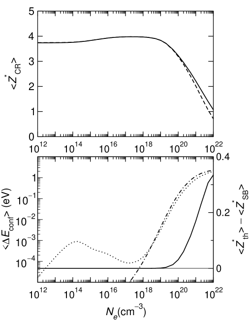
Figure 1: Upper part: Carbon plasma average charge in collisional-radiative model with configuration averaging (solid line) and detailed levels (broken line) as a function of electronic density for an electronic temperature $T_{e}=10\text{ eV}$. Lower part: averaged configuration energy dispersion as computed from (III.1) with collisional-radiative populations (dotted line, left scale) or with Saha-Boltzmann populations (dot-dash line, left scale); average-charge difference (III.3) between the modified CR system $<Z^{\star}_{\text{th}}>$ and the Saha-Boltzmann solution $<Z^{\star}_{\text{SB}}>$ (solid line, right scale), both computed in the configuration-average formalism.

On the upper part of Fig. 1, we have plotted the average ion charge $<Z^{\star}>$ versus the electron density at $T_{e}=10\text{ eV}$, both in the CA and in the detailed collisional-radiative formalism. Therefore, both should describe non-LTE effects and differ from the Saha-Boltzmann value, as analyzed in subsection III.4. As a rule, the CA procedure appears as pretty accurate, which is interesting since this average involves a much simpler matrix inversion. But a detailed inspection of Fig. 1 reveals some discrepancies, at low densities first (e.g., at $N_{e}=10^{13}\text{ cm}^{-3}$, $<Z^{\star}_{\text{CR}}>$ is 3.739 in the CA solution, and 3.749 in the detailed solution), and more prominently at densities above $N_{e}=10^{20}\text{ cm}^{-3}$: if $N_{e}=10^{21}\text{ cm}^{-3}$, $<Z^{\star}_{\text{CR}}>$ is 1.977 for the CA and 2.076 for the detailed level computation.

An intuitive explanation for this behavior is the following. In “coronal” plasmas at 10 eV, the most probable charge state is the He-like Cv and the most populated configuration is simply $1s^{2}$. At higher densities, recombination rates become larger and ions with a more complex structure dominate. Since these ions have configurations with a larger energy dispersion, the average configuration width may become of the order of magnitude of the thermal energy $k_{B}T_{e}$. Therefore the intuitive criterion for the validity of configuration averaging may be written as

$$<\Delta E>=\sum_{\alpha}N_{\alpha}\Delta E_{\alpha}\ll k_{B}T_{e}$$ (III.1)

where $N_{\alpha}$ is the $\alpha$-configuration population (with $\sum_{\alpha}N_{\alpha}=1$) and $\Delta E_{\alpha}$ is the energy dispersion

$$\Delta E_{\alpha}=\left(\frac{1}{g_{\alpha}}\sum_{i\in\alpha}g_{i}(E_{i}-E_{\alpha})^{2}\right)^{1/2}.$$ (III.2)

Unfortunately this criterion, though necessary, is far from sufficient. In the lower part of Fig. 1, two variants of the dispersion (III.1) are plotted: the dotted line corresponds to populations $N_{\alpha}$ computed using the collisional-radiative solution, the dash-dot line is obtained with $N_{\alpha}$ as given by the Saha-Boltzmann equation. Both values are significantly below 10 eV, by a factor of 7 at the minimum, even for large density values where one observes a small inaccuracy in the configuration average approximation. Moreover we will exhibit a much more severe breakdown of validity of the criterion (III.1) in the next section. However, in subsection II.2.2, we have shown that a useful test consists in performing a collisional-radiative analysis study with partial rates $R^{\prime}$ which should amount to the Saha-Boltzmann solution (i.e., LTE) if all levels in a given configuration had the same collision rates. Therefore, in the lower part of Fig. 1, the solid line is the difference

$$\Delta Z^{\star}=<Z^{\star}_{\text{th}}{}^{\text{config-av}}>-<Z^{\star}_{\text{SB}}{}^{\text{config-av}}>$$ (III.3)

where $<Z^{\star}_{\text{th}}{}^{\text{config-av}}>$ is the plasma charge computed with partial rates (II.7), while $<Z^{\star}_{\text{SB}}{}^{\text{config-av}}>$ is the plasma charge obtained through Saha-Boltzmann equation, both in a configuration-averaged formalism (remember that such figures are identical when one deals with detailed levels, cf. Table 2). One notices a significant average-charge difference of about 0.17 at $10^{21}\text{ electrons/cm}^{3}$. As mentioned in subsection II.2.2, the increase in the quantity (III.3) is a clear indication of the breakdown of the validity of the configuration average. The difference (III.3) is not a direct estimate of $<Z^{\star}_{\text{CR}}{}^{\text{config-av}}>-<Z^{\star}_{\text{CR}}{}^{\text{detailed}}>$ but a value of about 0.2 for the test (III.3) suggests a serious inaccuracy in the configuration-average approach.

III.4 Density dependence

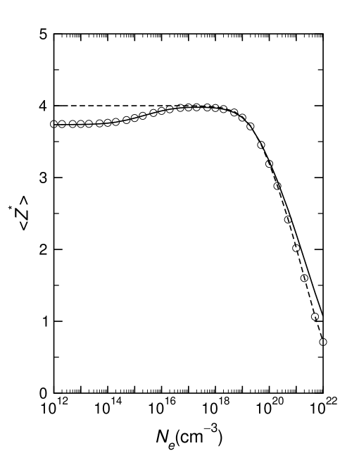
Figure 2: Carbon plasma average charge for $T_{e}=10\text{ eV}$. Solid line: collisional-radiative solution with configuration average, broken line: Saha-Boltzmann solution, circles: collisional-radiative solution with detailed levels.

In order to demonstrate non-LTE effects, we have plotted on Fig. 2 the configuration average charge of a 10 eV-carbon plasma, both within the present collisional-radiative model and using the Saha-Boltzmann equation, i.e., at LTE. Generally speaking, as the electron density $N_{e}$ increases, one expects that LTE will prevail because collisions will dominate radiative processes. At high $N_{e}$ the most probable process becomes three-body recombination since it is the only one depending on the square of the electron density, therefore one expects a decrease of $<Z^{\star}>$ as $N_{e}$ increases. This is visible on Fig. 2, which also shows that for $N_{e}<10^{16}\text{ cm}^{-3}$, the CR charge is lower than the LTE charge. In coronal plasmas, dominant processes are radiative recombination and collisional ionization: since the latter is balanced by three-body recombination while the former is not balanced by its inverse process (if photoionization with a thermal radiation at $T_{e}$ was present, this would ensure complete LTE) the “unbalanced” recombination process tends to lower the average ion energy and the average plasma charge. Then the CR solution converges toward LTE at $N_{e}\simeq 10^{18}\text{ cm}^{-3}$, as expected. A little more surprising is the divergence of the CR and LTE curves at higher densities $N_{e}>10^{21}\text{ cm}^{-3}$. Again, this arises from the limitation of validity of the configuration average, which may be observed for high densities $N_{e}$ as well as for low temperatures $T_{e}$ (Fig. 1). The detailed CR solution (circles on Fig.2) agrees with the configuration-average solution at low $Ne_{e}$, while for large $N_{e}$ it tends to the Saha-Boltzmann limit and differs from the configuration average.

IV Discussion of the configuration-average validity

IV.1 Analysis of the two validity criteria

We have demonstrated in the previous section that the energy criterion (III.1) is not sufficient to ensure the validity of the configuration-average procedure. A physical explanation for this is that while the condition (III.1) relies on energies only, the analysis using the partial rates equation and the estimate of the difference (III.3) involves the transition rates. Therefore both conditions are complementary, and the latter is certainly most stringent. Another indication that the departure of (III.3) from zero is a sign of dispersion in the transition probabilities relies on the analysis of the Saha-Boltzmann average charge difference $<Z^{\star}_{\text{SB}}{}^{\text{config-av}}>-<Z^{\star}_{\text{SB}}{}^{\text{detailed}}>$: as illustrated by Table 3, this quantity turns out to remain small (less than 0.1) even at low temperatures. This happens because the Saha-Boltzmann equation involves energies and not rates, and therefore is insensitive to the rate dispersion inside a configuration.

IV.2 Comparison with other data

Though the aim of this work was to analyze a validity criterion rather than to perform a reference CR calculation in carbon, it is instructive to compare the present results with some recent data. Colgan et al Colgan et al. (2006) have performed a detailed analysis of non-LTE carbon plasmas, both in the configuration average and in the “fine-structure”, i.e., detailed formalism. Their computation has been performed with the Cowan-based Los Alamos suite of codes and involves 1348 configurations and 24 902 levels, much is more than in the present work. Nevertheless, as seen in Table 4, their 10 eV-data compare satisfactorily with ours, whatever the density: the difference is less than 2%. This is a general trend in such a range of temperatures, where the carbon structure tends to the very stable ($Z^{\star}=4$) $1s^{2}$ configuration.

However, at 3 eV the difference within the detailed-formalism results remains reasonable (about 10%), while large discrepancies, sometimes by a factor of 2, are observed on the configuration-average results. It is somewhat expected that low-$T_{e}$ results exhibit large dispersion, as already noticed in the NLTE conferences Bowen et al. (2003, 2006): then the neutral or weakly charged ions become preponderant, and atomic models such as HULLAC are then known to be much less efficient; furthermore, collision cross-sections are usually bigger at low $T_{e}$ and inaccuracies such as those mentioned previously (Sec. II) have a strong influence. Nevertheless the factor of 2 on the configuration-average plasma charge needs further attention, and is thoroughly analyzed in subsection IV.4.

IV.3 Low-temperature behavior

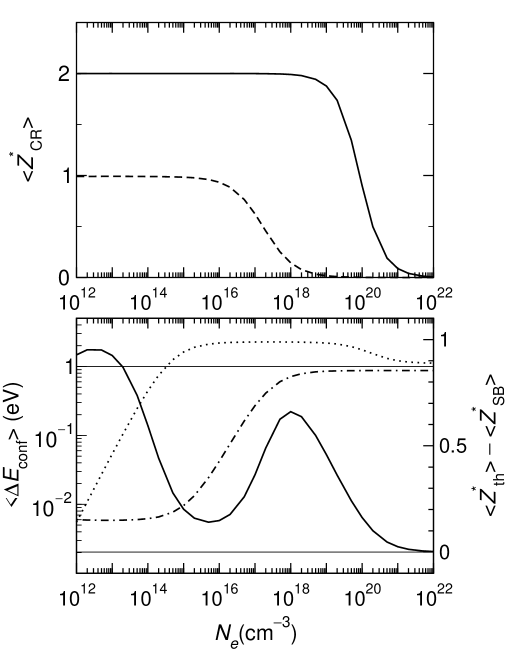
Figure 3: Same as figure 1, but for an electron temperature $T_{e}=\text{1 eV}$. Notice on the top subfigure the strong departure from the configuration-average validity if $N_{e}\leq 10^{14}\text{ cm}^{-3}$, which is not detected by the $<\Delta E_{\text{conf}}>$ criterion (bottom subfigure, dotted line), but is detected by the criterion on $<Z^{\star}_{\text{th}}>-<Z^{\star}_{\text{SB}}>$ (bottom subfigure, solid line).

An even more spectacular proof for the insufficiency of the energy condition is provided by the study of the carbon plasma at $T_{e}=1\text{ eV}$. The results are summarized in Fig. 3. It is noticeable that while the energy dispersion (III.1), plotted as dotted or dot-dash lines, is below $N_{e}=10^{14}\text{ cm}^{-3}$ less than $T_{e}$, and more than 2-order of magnitude less at $N_{e}=10^{12}\text{ cm}^{-3}$, the configuration average validity is always dubious then, as pointed out by the upper part of this figure. Conversely, as stressed before, when the criterion on $\Delta E$ is not sufficient, the $<Z^{\star}>$ values from the modified CR system and the Saha-Boltzmann solution are significantly different, indicating the breakdown of the configuration-average procedure. It appears on this example, considering, e.g., $N_{e}=10^{12}\text{ cm}^{-3}$ and $10^{22}\text{ cm}^{-3}$ that both criteria should be checked.

Comparing these data to those in Table 4, one notices that the low-density average charge in the detailed calculation increases with $T_{e}$ as expected, the $<Z^{\star}>\simeq 1$ at $T_{e}=1\text{ eV}$ being a plain coincidence; inversely, in configuration average the low-density charge turns out to be $<Z^{\star}>\simeq 2$ on a broad range of $T_{e}$. Of course the criterion (III.3) demonstrates that this value is unreliable, but this unexpected “stability” deserves a more detailed analysis.

IV.4 Breakdown of the configuration-average validity for cascade autoionization processes

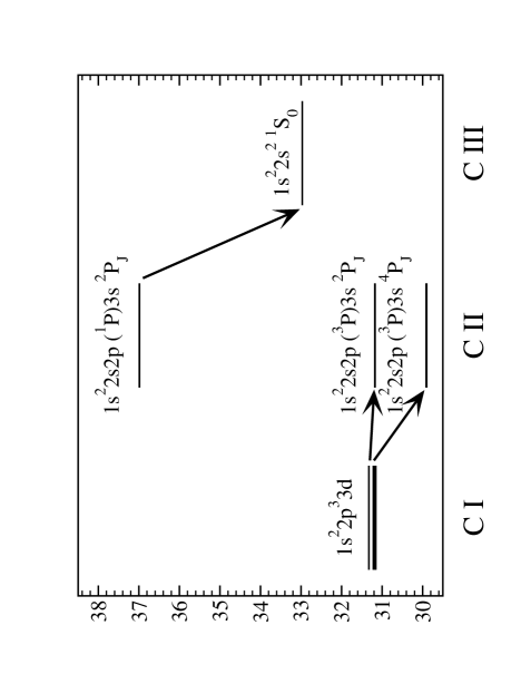
Figure 4: Autoionization processes involving three particular configurations in Ci, Cii, Ciii. The arrows indicate the dominant transitions accounted for in the present calculation. The vertical axis is the energy in eV, respective to the Ci ground state. Only some of the 38 levels of the $1s^{2}2p^{3}3d$ configuration are displayed. About ten of them autoionize toward the $1s^{2}2s2p\;({}^{3}P)3s\ {}^{2}P$ or the $1s^{2}2s2p\;({}^{3}P)3s\ {}^{4}P$ levels — which are below the Cii limit $1s^{2}2s^{2}\;{}^{1}S_{0}$ and do not themselves autoionize —, and none toward the upper levels ($1s^{2}2s2p\;({}^{1}P)3s\ {}^{2}P$), which are the only two levels in the configuration $1s^{2}2s2p3s$ that autoionize. No cascade autoionizing process exists from $1s^{2}2p^{3}3d$ to $1s^{2}2p^{2}$, though large average autoionization rates connect these configurations.

A thorough examination of the various-configuration influence has revealed that the unexpected low-$T_{e}$ low-$N_{e}$ configuration-averaged value $<Z^{\star}>\simeq 2$ arises mostly from two configurations, namely $1s^{2}2p^{3}3d$ in Ci and $1s^{2}2s2p3s$ in Cii. As a matter of fact, a simple model involving the five configurations $1s^{2}2s^{2}2p^{2}$, $1s^{2}2p^{3}3d$, $1s^{2}2s^{2}2p$, $1s^{2}2s2p3s$, and $1s^{2}2s^{2}$ fairly reproduces the unexpected behavior of Fig. 3. In a rather unusual way, the dominant transition rates are then the autoionization rates from some levels of the first configuration to some levels of the second one. Dielectronic recombination rates are accounted for here, but they are small because the electron density is low. As illustrated by Fig. 4, while the highest members of the $1s^{2}2p^{3}3d$ configuration decay to the $1s^{2}2s2p({}^{3}P)3s\,{}^{2}P$ doublet or to the $1s^{2}2s2p({}^{3}P)3s\,{}^{4}P$ quartet, all these levels lie below the Cii first ionization limit and do not autoionize; conversely, the upper member of this configuration, namely the $1s^{2}2s2p({}^{1}P)3s\,{}^{2}P$ doublet, does autoionize towards the Ciii ground state $1s^{2}2s^{2}\,{}^{1}S$ with a very large probability. So this detailed-level analysis shows that the cascade autoionization process $1s^{2}2p^{3}3d\rightarrow 1s^{2}2s2p3s\rightarrow 1s^{2}2s^{2}$ is not allowed. However, the configuration-average autoionization rates $1s^{2}2p^{3}3d\rightarrow 1s^{2}2s2p3s$ and $1s^{2}2s2p3s\rightarrow 1s^{2}2s^{2}$ are both very large ($6.8\times 10^{14}\text{ s}^{-1}$ and $3.6\times 10^{13}\text{ s}^{-1}$ respectively) and introduce a spurious very intense two-step transition from Ci to Ciii, which explains the very stable and large Ciii ground state population. The explanation why Colgan et al Colgan et al. (2006) did not notice such a big discrepancy as ours between the detailed and CA ionization stages at 3 eV appears now clearly: the $1s^{2}2p^{3}3d$ configuration was not accounted for in their calculation. Remarkably enough, adding or removing dozens of configurations other than the ones listed in Fig. 4 does not significantly change the average $Z^{\star}$ (CA or detailed), while a plain five-configuration model qualitatively reproduces the Fig. 3 behavior.

Though the $1s^{2}2p^{3}3d$ and $1s^{2}2s2p3s$ configurations have an energy dispersion $\Delta E_{\alpha}$ larger than $T_{e}$ (3.41 eV and 2.93 eV respectively) these configurations have very small populations ($9.7\times 10^{-16}$ and $8.8\times 10^{-11}$ respectively), therefore the criterion (III.1) is largely fulfilled. A more strict criterion such as $\max_{\alpha}(\Delta E_{\alpha})<k_{B}T_{e}$ could be proposed, but it would be hardly satisfied except at very large $T_{e}$ ($\max(\Delta E_{\alpha})=5.3\text{ eV}$ for the carbon configurations considered here), and furthermore one may question whether configurations with very small populations should contribute to this condition.

To conclude this low-$T_{e}$ analysis, it must be noted that the current computation generates levels from $1s^{2}2p^{3}3d$ and $1s^{2}2s2p3s$ configurations at very close energies (explaining the large autoionization rate as is usual for this process), which may not be reproduced by more accurate computations or other atomic models. Concerning experimental data, in the NIST (National Institute of Standards and Technology) tables NIS (2006), one finds the $1s^{2}2s2p({}^{3}P)3s$ levels (but not the $2s2p({}^{1}P)3s$ ones), while the highly excited configuration $1s^{2}2p^{3}3d$ is absent; the agreement on the $1s^{2}2s2p({}^{3}P)3s$ level positions is good. Noticeably, most of the autoionizing states considered here are absent in the NIST tables, probably because their broadening makes their position difficult to report. Nevertheless, the present analysis is useful in itself because the reported effect must happen in other configurations or ions as soon as these quasi-degeneracies are indeed present.

V Conclusion

This work initially stemmed from the need of a collisional-radiative solver (or postprocessor) for the HULLAC code; at the time of writing it, such solver was not part of the HULLAC suite, at least in the publicly distributed code. Few CR computations based on the HULLAC suite have appeared recently Chung et al. (2006). The possibility of performing the configuration average makes the handling of the CR equations considerably easier, the system size decreasing from 1781 to 149 in the analyzed carbon case. Superconfiguration codes Hansen et al. (2006) provide an interesting alternative concerning the computation efficiency and their ability to deal with complex atoms. However the inclusion in these formalisms of effects such as a full configuration interaction is still lacking. Of course the detailed-level methods will for long suffer from the considerable computing time, considering that the carbon plasma case analyzed here is one of the simplest. In this work we have proposed a method to check the validity of the configuration average procedure which goes far beyond the plain criterion on energy dispersion. It involves the solution of two configuration-averaged CR systems instead of one, but this is much less cumbersome than solving a detailed-level CR system. This criterion is based on rate equations for collisional excitation and ionization and their reverse processes, and is therefore sensitive to a possible non-uniformity inside a configuration of these rates only. However, it may be generalized to include other processes, for instance the radiative processes, provided that one accounts for absorption and spontaneous emission from a fictitious Planck radiation field in thermal equibrium with the electrons. In the analyzed case of cascade autoionization processes, it has been demonstrated that a spectacular breakdown of the configuration-average validity may occur which can only be detected using the criterion proposed here. Finally, the present formalism should also be efficient in computing other physical quantities such as the opacity, the emissivity Colgan et al. (2006) or radiative cooling coefficients Chung et al. (2006) of non-LTE plasmas; such a topic has been recently addressed in our laboratory de Gaufridy de Dortan (2006).

Appendix A The averaged collisional-radiative equations

Rate equations for detailed levels $i$ belonging to a given configuration $\alpha$ are written as (II.5) while their configuration average is defined as

$$\frac{dN_{\alpha}}{dt}=\sum_{\beta}R_{\beta\alpha}N_{\beta}-N_{\alpha}\sum_{\beta}R_{\alpha\beta}$$ (A.1)

where the configuration population is $N_{\alpha}=\sum_{i\in\alpha}N_{i}$ and the transition rates from configuration $\alpha$ to $\beta$ writes

$$R_{\alpha\beta}=\frac{1}{g_{\alpha}}\sum_{i\in\alpha}\sum_{j\in\beta}g_{i}R_{ij}$$ (A.2)

$g_{\alpha}$ being the degeneracy $\sum_{i\in\alpha}g_{i}$ of the initial configuration.

Appendix B Checking the numerical CR system solution

The CR analysis in the detailed-level case (II.6) or its configuration-average counterpart requires the solution of a potentially very large system of linear equations. One should therefore check the numerical accuracy of this procedure. In this CR system, the $R_{ij}$ stand for all the transitions processes enumerated in section II.1. Because no external electromagnetic field is present, two of these processes are not balanced by their inverse processes: radiative deexcitation and radiative recombination. In order to check the accuracy of these CR equations, one substitutes partial rates $R^{\prime}_{ij}$ to the full rates $R_{ij}$, which only include collisional excitation, collisional ionization and their inverse processes.

In the detailed-level case, since the effects accounted for by rates $R^{\prime}$ obey the detailed-balance principle, the correct numerical solution of this system — numerically as complex as the original system since the same number of equations is involved — must be the Saha-Boltzmann solution.

In the configuration-average case, the comparison of this solution to the Saha-Boltzmann solution with averaged energies provides a validity check of the CR solution as discussed, e.g., in subsection III.3.

Tables

Table 1: List of configurations included in the HULLAC-based collisional-radiative analysis of a carbon plasma. $[1s^{2}]$ means unrepeated identical core. One has $3\leq N\leq 5,0\leq l\leq N-1$ for each charge state. $N_{\text{conf}}$ is the number of configurations, $N_{\text{lev}}$ the number of (relativistic) levels.

Charge	Configurations	$N_{\text{conf}}$	$N_{\text{lev}}$
Ci	$[1s^{2}]\ 2s^{2}2p^{2},\ 2s2p^{3},\ 2p^{4},\ 2s^{2}2pNl,\ 2s2p^{2}Nl,\ 2p^{3}Nl$	39	1004
Cii	$[1s^{2}]\ 2s^{2}2p,\ 2s2p^{2},\ 2p^{3},\ 2s^{2}Nl,\ 2s2pNl,\ 2p^{2}Nl$	39	513
Ciii	$[1s^{2}]\ 2s^{2},\ 2s2p,\ 2p^{2},\ 2sNl,\ 2pNl$	27	166
Civ	$[1s^{2}]\ 2s,\ 2p,\ Nl$	14	24
Cv	$1s^{2},\ 1s2s,\ 1s2p,\ 1sNl$	15	49
Cvi	$1s,\ 2s,\ 2p,\ Nl$	15	25
Cvii		1	1
Total		150	1782

Table 2: Accuracy check of the collisional-radiative (CR) detailed-level solution for carbon at $T_{e}=10\text{ eV}$. The average $<Z^{\star}_{\text{th}}>$ is the ion charge obtained by solving the modified CR system (II.7), and should be equal to $<Z^{\star}_{\text{SB}}>$, the average ion charge derived from Saha-Boltzmann equation, for infinite numerical accuracy. The additional test $\delta_{\text{max}}$ is the maximum difference on the ion-level populations between this modified CR system and the Saha-Boltzmann solution.

$N_{e}\text{(cm${}^{-3}$)}$	$<Z^{\star}_{\text{th}}>$	$<Z^{\star}_{\text{SB}}>$	$\delta_{\text{max}}$
$10^{12}$	4.000004022	4.000004022	$7.7\times 10^{-14}$
$10^{14}$	3.999998278	3.999998278	$3.2\times 10^{-14}$
$10^{16}$	3.999823805	3.999823805	$3.3\times 10^{-12}$
$10^{18}$	3.982612437	3.982612437	$3.2\times 10^{-10}$
$10^{20}$	3.192620512	3.192620504	$4.8\times 10^{-9}$
$10^{22}$	0.711283477	0.711283469	$3.8\times 10^{-10}$

Table 3: Average carbon plasma charge from Saha-Boltzmann equation at $T_{e}=10\text{ eV}$: configuration-average and detailed-level values.

$N_{e}\text{(cm${}^{-3}$)}$	$<Z^{\star}_{\text{SB}}{}^{\text{config-av}}>$	$<Z^{\star}_{\text{SB}}{}^{\text{detailed}}>$
$10^{12}$	4.000004	4.000004
$10^{13}$	4.000000	4.000000
$10^{14}$	3.999998	3.999998
$10^{15}$	3.999982	3.999982
$10^{16}$	3.999824	3.999824
$10^{17}$	3.998240	3.998240
$10^{18}$	3.982613	3.982612
$10^{19}$	3.844529	3.844448
$10^{20}$	3.194906	3.192621
$10^{21}$	2.026326	2.017892
$10^{22}$	0.717721	0.711283

Table 4: Average ionization of a carbon plasma: Colgan et al Colgan et al. (2006) and present work. The Colgan’s “fine-structure” (FS) is a detailed formalism, CA is the configuration average in both works.

$T_{e}\text{(eV)}$	$N_{e}\text{(cm${}^{-3}$)}$	Colgan et al		This work
		FS	CA	detailed	CA
3	$10^{13}$	1.730	1.486	1.902	1.999
	$10^{15}$	1.923	1.895	2.037	2.166
	$10^{17}$	1.952	1.948	1.991	2.501
	$10^{19}$	1.004	0.959	1.179	1.980
10	$10^{13}$	3.723	3.701	3.746	3.739
	$10^{15}$	3.862	3.856	3.828	3.828
	$10^{17}$	3.979	3.978	3.976	3.976
	$10^{19}$	3.786	3.785	3.833	3.835

Figures

References

- Bauche-Arnoult et al. (1979) C. Bauche-Arnoult, J. Bauche, and M. Klapisch, Phys. Rev. A 20, 2424 (1979).
- Bauche-Arnoult et al. (1982) C. Bauche-Arnoult, J. Bauche, and M. Klapisch, Phys. Rev. A 25, 2641 (1982).
- Bauche et al. (1988) J. Bauche, C. Bauche-Arnoult, and M. Klapisch, Adv. At. Mol. Phys. 23, 131 (1988).
- Bauche-Arnoult et al. (1985) C. Bauche-Arnoult, J. Bauche, and M. Klapisch, Phys. Rev. A 31, 2248 (1985).
- Bar-Shalom et al. (1989) A. Bar-Shalom, J. Oreg, W. H. Goldstein, D. Shvarts, and A. Zigler, Phys. Rev. A 40, 3183 (1989).
- Busquet (1993) M. Busquet, Phys. Fluids B 5, 4191 (1993).
- Bauche and Bauche-Arnoult (2000) J. Bauche and C. Bauche-Arnoult, J. Phys. B 33, L283 (2000).
- Poirier et al. (2006) M. Poirier, T. Blenski, F. de Gaufridy de Dortan, and F. Gilleron, J. Quant. Spectrosc. Radiat. Transfer 99, 482 (2006).
- Colombant and Tonon (1973) D. Colombant and G. F. Tonon, J. Appl. Phys. 44, 3524 (1973).
- Bates et al. (1962) D. R. Bates, A. E. Kingston, and R. W. P. McWhirter, Proc. R. Soc. London, Ser. A 267, 297 (1962).
- McWhirter (1978) R. W. P. McWhirter, Phys. Rep. 37, 165 (1978).
- Faussurier et al. (2001) G. Faussurier, C. Blancard, and E. Berthier, Phys. Rev. E 63, 026401 (2001).
- Bar-Shalom et al. (1997) A. Bar-Shalom, J. Oreg, and M. Klapisch, Phys. Rev. E 56, R70 (1997).
- Bar-Shalom et al. (2000) A. Bar-Shalom, J. Oreg, and M. Klapisch, J. Quant. Spectrosc. Radiat. Transfer 65, 43 (2000).
- Peyrusse (2001) O. Peyrusse, J. Quant. Spectrosc. Radiat. Transfer 71, 571 (2001).
- Bauche et al. (2004) J. Bauche, C. Bauche-Arnoult, and K. B. Fournier, Phys. Rev. E 69, 026403 (2004).
- Hansen et al. (2006) S. Hansen, K. B. Fournier, C. Bauche-Arnoult, J. Bauche, and O. Peyrusse, J. Quant. Spectrosc. Radiat. Transfer 99, 272 (2006).
- Rodríguez et al. (2006) R. Rodríguez, J. Gil, R. Florido, J. Rubiano, P. Martel, and E. Mínguez, J. Phys. IV 133, 981 (2006).
- Bowen et al. (2003) C. Bowen, A. Decoster, C. J. Fontes, K. B. Fournier, O. Peyrusse, and Y. Ralchenko, J. Quant. Spectrosc. Radiat. Transfer 81, 71 (2003).
- Bowen et al. (2006) C. Bowen, R. W. Lee, and Y. Ralchenko, J. Quant. Spectrosc. Radiat. Transfer 99, 102 (2006).
- Nishihara et al. (2006) K. Nishihara, A. Sasaki, A. Sunahara, and T. Nishikawa, EUV Sources for Lithography (SPIE Press, Bellingham, Washington USA, 2006), chap. 11, pp. 339–370.
- O’Sullivan et al. (2006) G. O’Sullivan, A. Cummings, P. Dunne, P. Hayden, L. McKinney, N. Murphy, and J. White, EUV Sources for Lithography (SPIE Press, Bellingham, Washington USA, 2006), chap. 5, pp. 149–173.
- Al Rabban et al. (2006) M. Al Rabban, M. Richardson, H. Scott, F. Gilleron, M. Poirier, and T. Blenski, EUV Sources for Lithography (SPIE Press, Bellingham, Washington USA, 2006), chap. 10, pp. 299–337.
- Gilleron et al. (2003) F. Gilleron, M. Poirier, T. Blenski, M. Schmidt, and T. Ceccotti, J. Appl. Phys. 94, 2086 (2003).
- Bauche et al. (1991) J. Bauche, C. Bauche-Arnoult, and M. Klapisch, J. Phys. B 24, 1 (1991).
- Bar-Shalom et al. (2001) A. Bar-Shalom, M. Klapisch, and J. Oreg, J. Quant. Spectrosc. Radiat. Transfer 71, 169 (2001).
- Cowan (1981) R. D. Cowan, The theory of atomic structure and spectra (University of California Press, Berkeley, California, 1981).
- Gu (2001) M. F. Gu, The flexible atomic code, http://asc.harvard.edu/fellows/viewgraphs/2001/gu/gu2.ps (2001).
- Gu (2003) M. F. Gu, Astrophys. J. 582, 1241 (2003).
- Goett et al. (1980) S. J. Goett, R. E. H. Clark, and D. H. Sampson, At. Data Nucl. Data Tables 25, 185 (1980).
- Sampson et al. (1983) D. H. Sampson, S. J. Goett, and R. E. H. Clark, At. Data Nucl. Data Tables 29, 467 (1983).
- Fontes et al. (1993) C. J. Fontes, D. H. Sampson, and H. L. Zhang, Phys. Rev. A 48, 1975 (1993).
- van Regemorter (1962) H. van Regemorter, Astrophys. J. 136, 906 (1962).
- Mewe (1972) R. Mewe, Astron. Astrophys. 20, 215 (1972).
- Burgess and Tully (1992) A. Burgess and J. A. Tully, Astron. Astrophys. 254, 436 (1992).
- Colgan et al. (2006) J. Colgan, C. J. Fontes, and J. Abdallah Jr., High Energy Density Physics 2, 90 (2006).
- NIS (2006) NIST Atomic Spectra Database, http://physics.nist.gov/PhysRefData/ASD/index.html (2006).
- Chung et al. (2006) H. K. Chung, K. B. Fournier, and R. W. Lee, High Energy Density Physics 2, 7 (2006).
- de Gaufridy de Dortan (2006) F. de Gaufridy de Dortan, Tech. Rep. CEA-R-6115, CEA (2006).