Two-dimensional multisolitons and azimuthons in Bose-Einstein condensates with attraction

Abstract

We present spatially localized nonrotating and rotating (azimuthon) multisolitons in the two-dimensional (2D) (”pancake-shaped configuration”) Bose-Einstein condensate (BEC) with attractive interaction. By means of a linear stability analysis, we investigate the stability of these structures and show that rotating dipole solitons are stable provided that the number of atoms is small enough. The results were confirmed by direct numerical simulations of the 2D Gross-Pitaevskii equation.

Localized coherent structures, such as fundamental solitons, vortices, nonrotating and rotating multisolitons are universal objects which appear in many nonlinear physical systems Kivshar1 , and, in particular, in Bose-Einstein condensates (BEC’s). Stability of these nonlinear structures is one of the most important questions because of its direct connection with the possibility of experimental observation of solitons and vortices.

Detailed investigations of the stability of localized vortices in an effectively two-dimensional (2D) trapped BEC with a negative scattering length (attractive interaction) were performed in Ref.  Malomed and later extended to the three-dimensional case Malomed2 (see also Ref. Saito ). While vortex solitons in attractive BEC are strongly unstable in free space, the presence of the trapping potential results in existence of stable vortices provided that the number of particles does not exceed a threshold value Malomed ; Saito ; Berge .

Recently, a novel class of 2D spatially localized vortices with a spatially modulated phase, the so called azimuthons, was introduced in Ref. Kivshar2 . Azimuthons represent intermediate states between the radially symmetric vortices and rotating soliton clusters. In contrast to the linear vortex phase, the phase of the azimuthon is a staircaselike nonlinear function of the polar angle. Various kinds of azimuthons have been shown to be stable in media with a nonlocal nonlinear response Lopez1 ; Lopez2 ; Skupin ; We2 ; We3 .

The aim of this Brief Report is to present nonrotating multisoliton (in particular, dipole and quadrupole) and rotating multisoliton (azimuthon) structures in the 2D BEC with attraction and study their stability by a linear stability analysis. We show that, in the presence of a confining potential, stable azimuthons also exist for a medium with a local cubic attractive nonlinearity. Results of the linear stability analysis were confirmed by direct numerical simulations of the azimuthon dynamics.

We consider a condensate which is loaded in an axisymmetric with respect to the $(x,y)$ plane harmonic trap, and tightly confined in the $z$ direction. The dynamics of the condensate is described by the Gross-Pitaevskii equation (GPE)

$$i\hbar\frac{\partial\Psi}{\partial t}=\left\{-\frac{\hbar^{2}}{2m}\Delta+\frac{m}{2}[\Omega_{r}^{2}(x^{2}+y^{2})+\Omega_{z}^{2}z^{2}]\right.$$

$$\left.+\frac{4\pi\hbar^{2}a}{m}|\Psi|^{2}\right\}\Psi,$$ (1)

where $\Psi(\mathbf{r},t)$ is the condensate wave function, $a\gtrless 0$ is the $s$-wave scattering length. We assume that the axial confinement frequency $\Omega_{z}$ is much larger than the radial one $\Omega_{r}$ (the pancake configuration). Then, the 3D equation (1) can be reduced to an effective GPE in two dimensions Malomed (for a detailed discussion of the applicability of the 2D approximation see Ref. Malomed ). The standard reduction procedure Salasnich ; Louis leads to the following 2D equation

$$i\frac{\partial\psi}{\partial t}=-\Delta_{\perp}\psi+\frac{\Omega_{0}^{2}}{4}(x^{2}+y^{2})\psi-\sigma|\psi|^{2}\psi,$$ (2)

where appropriate dimensionless units are used, and $\Delta_{\perp}=\partial/\partial x^{2}+\partial/\partial y^{2}$, $\sigma=\pm 1$, where the $+(-)$ sign corresponds to attractive (repulsive) contact interaction.

Equation (2) conserves the 2D norm (the normalized number of particles)

$$N=\int|\psi|^{2}dxdy,$$ (3)

and energy

$$E=\int\left\{|\nabla_{\perp}\psi|^{2}+\frac{\Omega_{0}^{2}}{4}(x^{2}+y^{2})|\psi|^{2}-\frac{\sigma}{2}|\psi|^{4}\right\}dxdy$$ (4)

Stationary solutions of Eq. (2) in the form

$$\psi(x,y,t)=\varphi(x,y)\exp(-i\mu t),$$ (5)

where $\mu$ is the chemical potential, resolve the variational problem $\delta S=0$ for the functional

$$S=E-\mu N.$$ (6)

Following Ref. Berge , let us consider the trial function $\varphi=A\phi_{a}(r/a,\theta)$, where $\phi_{a}$ is some test function, $A$ and $a$ is the amplitude and characteristic width of the stationary state, respectively. Then, the functional $S$ takes the form

$$S(a,A)=\alpha A^{2}-\beta A^{4}a^{2}+\frac{\Omega_{0}^{2}}{4}\gamma A^{2}a^{4}-\mu\delta A^{2}a^{2},$$ (7)

where the integral coefficients are

$$\alpha=\int|\nabla_{\vec{\xi}}\,\phi_{a}|^{2}d\vec{\xi},\quad\beta=\frac{\sigma}{2}\int|\phi_{a}|^{4}d\vec{\xi},$$ (8)

$$\delta=\int|\phi_{a}|^{2}d\vec{\xi},\quad\gamma=\int\xi^{2}|\phi_{a}|^{2}d\vec{\xi}.$$ (9)

The Euler-Lagrange equations $\partial S/\partial a=0$ and $\partial S/\partial A=0$ for the functional Eq. (7) give expressions for the width $a$ and amplitude $A$ Berge

$$a^{2}(\mu)=\frac{2\sqrt{\mu^{2}\delta^{2}+3\alpha\gamma\Omega_{0}^{2}}+2\mu\delta}{3\Omega_{0}^{2}\gamma}$$ (10)

$$A^{2}(\mu)=\frac{\Omega_{0}^{2}a^{2}\gamma-2\mu\delta}{2\beta}$$ (11)

The 2D norm $N$ and energy $E$ then read

$$N(\mu)=A^{2}(\mu)a^{2}(\mu)\delta=\frac{\delta a^{2}(\mu)}{2\beta}(\Omega_{0}^{2}a^{2}\gamma-2\mu\delta),$$ (12)

$$E(\mu)=\frac{A^{2}(\mu)a^{4}(\mu)}{2}\Omega_{0}^{2}\gamma.$$ (13)

In the following, we consider attractive short-range interactions and set $\sigma=1$. It then follows from Eq. (11) that solutions exist provided that the chemical potential $\mu$ does not exceed a critical value $\mu^{\ast}$ Berge ,

$$\mu\leq\mu^{\ast}=\frac{\Omega_{0}}{\delta}\sqrt{\alpha\gamma}.$$ (14)

To proceed further, we take a test function $\phi_{a}$ in the form

$$\phi_{a}(\vec{\xi})=\xi^{m}L_{n}^{(m)}(\xi^{2})e^{-\xi^{2}/2}(\cos m\theta+i\,p\sin m\theta),$$ (15)

where $m$ is an integer, $\theta$ is the azimuthal angle, $0\leqslant p\leqslant 1$, and $L_{n}^{(m)}(x)$ is the $n$th (i. e. with $n$ zeros) generalized Laguerre polynomial. The parameter $p$ determines the modulation depth of the soliton intensity. Note that the case $p=0$ corresponds to the nonrotating multisolitons (e. g. $m=1$ to a dipole, $m=2$ to a quadrupole etc.), while the opposite case $p=1$ corresponds to the radially symmetric vortices. The intermediate case $0<p<1$ corresponds to the rotating azimuthons. Since the vortices and azimuthons have a nontrivial phase, they carry out the nonzero $z$-component of the angular momentum

$$M_{z}=\mathrm{Im}\,\int\left[\psi^{\ast}(\mathbf{r}\times\nabla_{\perp}\psi)\right]_{z}dx\,dy,$$ (16)

which can be expressed as

$$M_{z}(\mu)=\frac{2pm}{(p^{2}+1)}N(\mu).$$ (17)

When $n\neq 0$, the ansatz Eq. (15) represents a rather exotic structure with $n$ nodes.

Inserting Eq. (15) into Eqs. (8) and (9), one can determine the coefficients $\alpha$, $\beta$, $\gamma$ and $\delta$. For the nodeless case ($n=0$) we have

$$\alpha_{0}^{(m)}=\gamma_{0}^{(m)}=\frac{\pi}{2}(p^{2}+1)(m+1)!,$$ (18)

$$\beta_{0}^{(m)}=\frac{\pi}{2^{m+5}}(3p^{4}+2p^{2}+3)(2m)!,$$ (19)

$$\delta_{0}^{(m)}=\frac{\pi}{2}(p^{2}+1)m!.$$ (20)

For the structures with one node ($n=1$), one can obtain

$$\alpha_{1}^{(m)}=\frac{\pi(m+3)}{2}(p^{2}+1)(m+1)!,$$ (21)

$$\beta_{1}^{(m)}=\frac{\pi(3m^{2}+5m+2)}{2^{2m+7}}(3p^{4}+2p^{2}+3)(2m)!,$$ (22)

$$\delta_{1}^{(m)}=\frac{\pi}{2}(p^{2}+1)(m+1)!,$$ (23)

$$\gamma_{1}^{(m)}=\frac{\pi}{2(m+2)}(p^{2}+1)(m+3)!.$$ (24)

Substituting Eqs. (18)–(20) or Eqs. (21)–(24) into Eqs. (10) and (11), we get the width and amplitude of the corresponding nonlinear structures. In what follows we restrict ourselves to the case of the nodeless states ($n=0$) and, in addition, set $\Omega_{0}=2$.

The dependences $\mu(N)$ and $E(N)$ obtained from Eqs. (12) and (13) for different values $p$ are plotted in Fig. 1 for $m=1$ and $m=2$. The curve $4$ corresponding radially symmetric vortices $p=1$ coincides with that obtained in Ref. Malomed ; Berge . It follows from Eq. (14) that the critical value for the chemical potential is $\mu^{\ast}=2(m+1)$ and does not depend on $p$. The asymptotic values $N_{max}(\mu=-\infty)$, which determine the (formal) collapse threshold, decrease with decreasing $p$. Results of the variational analysis are found to be in good agreement with numerical simulations (see below).

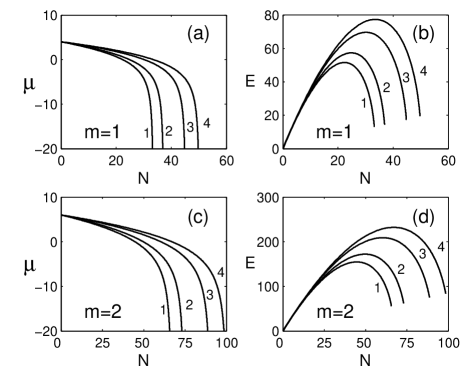
Figure 1: (a) Chemical potential $\mu$ and (b) energy $E$ versus normalized number of atoms $N$ for variational nodeless ($n=0$) solutions Eq. (15) with $p=0$ (curve $1$), $p=0.3$ (curve $2$), $p=0.6$ (curve $3$), and $p=1$ (curve $4$) for $m=1$; (c) and (d) the same for $m=2$.

Generally speaking, using the relaxation technique similar to one described in Ref. Petviashvili and choosing an appropriate initial guess, one can find numerically vortex and azimuthon solutions of Eq. (2) on Cartesian grid. Under this, the parameter $p$ (modulational depth), which is similar to the one in Eq. (15), can be introduced in the following way:

$$p=\max|\mathrm{Im}\,\Psi|/\max|\mathrm{Re}\,\Psi|.$$ (25)

However, the choice of initial guess (to achieve convergence) is extremely difficult and time consuming, and, moreover, we were not able to find azimuthon solutions with arbitrary $p$. Instead, we use an approximate but much simpler variational approach and introduce the following ansatz in polar coordinates $(r,\theta)$ Lopez1

$$\psi(\mathbf{r},t)=U(r)(\cos m\theta+i\,p\sin m\theta)e^{-i\mu t},$$ (26)

where $U(r)$ is a real function. Inserting the ansatz (26) into the action Eq. (6), integrating over $\theta$, but keeping an arbitrary dependence $U(r)$, one can then obtain the corresponding Euler-Lagrange equation,

$$\frac{d^{2}U}{dr^{2}}+\frac{1}{r}\frac{dU}{dr}+\left(\mu-r^{2}-\frac{m^{2}}{r^{2}}\right)U+f(p)U^{3}=0,$$ (27)

where

$$f(p)=\frac{3p^{4}+2p^{2}+3}{4(p^{2}+1)}.$$ (28)

Equation (27) was solved numerically with boundary conditions $U\rightarrow r^{|m|}$ at $r\rightarrow 0$, and $U\rightarrow 0$ at $r\rightarrow\infty$. In Fig. 2 we demonstrate an example of the azimuthon with two intensity peaks (i. e. with the topological charge $m=1$), $p=0.7$, and $\mu=2.7$. For fixed chemical potential $\mu$ and integer $m$, there is a family of azimuthon solutions with different $p$. Note that the ansatz (26) represents only particular class of the azimuthons. More general form of the azimuthon solutions, which are characterized by two independent integer numbers (number of peaks is generally independent on the topological charge $m$), was introduced in Ref. Kivshar2 .

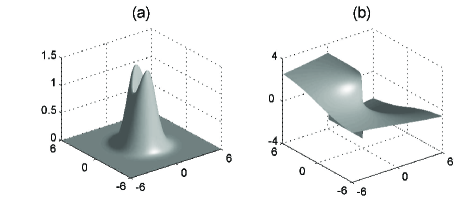
Figure 2: (a) Amplitude $|\varphi|$ and (b) phase $\arg\varphi$ distributions of the azimuthon with two intensity peaks ($m=1$) and $p=0.7$, $\mu=2.7$.

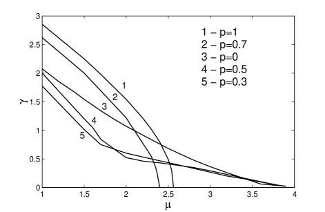
Figure 3: The growth rates $\gamma$ as functions of the chemical potential $\mu$ for $m=1$ and different $p$.

To study the stability of the stationary solutions, we represent the wave function in the form

$$\psi(\mathbf{r},t)=[\varphi_{0}(\mathbf{r})+\varepsilon(\mathbf{r},t)]e^{-i\mu t},$$ (29)

where the stationary solution $\varphi_{0}$ is perturbed by a small perturbation $\varepsilon$. As usual, one could then take

$$\varepsilon(\mathbf{r},t)=\varphi_{+}(\mathbf{r})e^{i\omega t}+\varphi_{-}^{\ast}(\mathbf{r})e^{-i\omega t},$$ (30)

and consider the corresponding eigenvalue problem, but, in our case with $p\neq 1$, this approach turns out to be ineffective. Indeed, the linearization of Eq. (2) around $\varphi_{0}$ in $\varepsilon$ leads to the eigenvalue problem

$$\hat{T}\varphi_{+}+\varphi_{0}^{2}\varphi_{-}=\omega\varphi_{+},$$ (31)

$$-\hat{T}\varphi_{-}-\varphi_{0}^{\ast\,2}\varphi_{+}=\omega\varphi_{-},$$ (32)

where $\hat{T}=\mu+\Delta_{\perp}-(x^{2}+y^{2})+2|\varphi_{0}|^{2}$ and $\omega$ are eigenvalues. Nonzero imaginary parts in $\omega$ imply the instability of the state $\varphi_{0}(\mathbf{r})$ with $\max|\mathrm{Im}\,\omega|$ being the instability growth rate. For radially symmetric vortices with $p=1$, azimuthal perturbations turn out to be the most dangerous, and the problem Eqs. (31) and (32) can be reduced to 1D (radial) one and can then be easily solved with high accuracy Malomed . The situation, however, changes dramatically for $p\neq 1$. In this case the radial symmetry is absent, and one must solve the full 2D eigenvalue problem. The problem on a $N\times N$ spatial grid implies a $2N^{2}\times 2N^{2}$ complex nonsymmetric matrix and, for reasonable $N$ (say, $N>200$), represents a formidable task. Instead, after inserting Eq. (29) into Eq. (2), we solved the Cauchy problem for the linearized equation

$$i\frac{\partial\varepsilon}{\partial t}+\mu\varepsilon+\Delta_{\perp}\varepsilon-(x^{2}+y^{2})\varepsilon+2|\varphi_{0}|^{2}\varepsilon+\varphi_{0}^{2}\varepsilon^{\ast}=0$$ (33)

with some initial perturbations $\varepsilon$. The final results are not sensitive to the specific form of $\varepsilon(x,y,0)$. If the dynamics is unstable, the corresponding solutions $\varepsilon(x,y,t)$, undergoing, generally speaking, oscillations, grow exponentially in time and an estimate for the growth rate $\gamma$ can be written as

$$\gamma=\frac{1}{2\Delta t}\ln\left\{\frac{P(t+\Delta t)}{P(t)}\right\},$$ (34)

where $P(t)=\int|\varepsilon|^{2}dxdy$, $t$ and $\Delta t$ are assumed to be large enough.

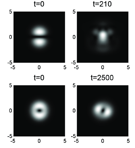
Figure 4: Top row – unstable dynamics of the dipole $p=0$ with $\mu=3.3$; bottom row – stable evolution of the azimuthon with $m=1$, $p=0.7$, and $\mu=2.7$.

In Fig. 3 we plot the growth rates $\gamma$ as functions of the chemical potential $\mu$ for $m=1$ and several different values of $p$. The case $p=1$ corresponds to radially symmetric vortices with the topological charge $m=1$ and was investigated in detail in Ref. Malomed . The corresponding curve in Fig. 3 coincides with that obtained in Ref. Malomed . The linear stability analysis shows that for solutions with $m=1$ and $p\lesssim 0.7$, the growth rate of perturbations $\gamma\neq 0$ for all $\mu$ so that there is no the stability region. The situation, however, changes when $p\gtrsim 0.7$. Under this, the growth rate of perturbations $\gamma=0$ if the chemical potential exceeds some critical value $\mu_{c}$. The stability window appears and the azimuthons with $p\gtrsim 0.7$ and $\mu_{c}<\mu<4$. The critical value $\mu_{c}$ monotonically increases from $\mu_{c}\sim 2.45$ (for $p=0.7$) to $\mu_{c}\sim 2.6$ (for $p=1$). All solutions with $m=2$ turn out to be unstable (for $p=1$ it was shown in Ref. Malomed ).

To verify the results of the linear analysis, we solved numerically the dynamical equation (2) initialized with our computed solutions with added Gaussian noise. The initial condition was taken in the form $\varphi_{0}[1+\nu\xi(x,y)]$, where $\varphi_{0}(x,y)$ is the numerically calculated solution, $\xi(x,y)$ is the white gaussian noise with variance $\sigma^{2}=1$ and the parameter of perturbation $\nu=0.005\div 0.1$. The unstable dynamics of the nonrotating dipole ($p=0$) with $\mu=3.3$ is illustrated in the top row of Fig.4. Stable evolution of the azimuthon with $p=0.7$ and $\mu=2.7$ (i. e. in the region of the stability) is shown in the bottom row of Fig.4. The azimuthon cleans up itself from the noise and survives over hundreds of the rotational periods.

In conclusion, we have presented nonrotating and rotating (azimuthon) multisolitons in an effectively 2D (”pancake-shaped configuration”) Bose-Einstein condensate with attractive interaction and parabolic trapping potential. We have performed a linear stability analysis of these structures and demonstrated that azimuthons with two intensity peaks (rotating dipoles) and with not too small modulational depth can be stable if the number of particles is below some critical value. The nonrotating multisolitons (dipoles and all high-order multipoles) appear to be unstable.

The author thanks Yu. A. Zaliznyak and A. I. Yakimenko for discussions.

References

- (1) See, e.g., Yu. S. Kivshar and G. Agrawal, Optical Solitons: From Fibers to Photonic Crystals (Academic Press, San Diego, 2003) and references therein.
- (2) D. Mihalache, D. Mazilu, B. A. Malomed, and F. Lederer, Phys. Rev. A 73, 043615 (2006).
- (3) B. A. Malomed, F. Lederer, D. Mazilu, and D. Mihalache, Phys. Lett. A 361, 336 (2007).
- (4) H. Saito, and M. Ueda, Phys. Rev. A 69, 013604 (2004).
- (5) T. J. Alexander and L. Bergé, Phys. Rev. E 65, 026611 (2002).
- (6) A. S. Desyatnikov, A. A. Sukhorukov, and Yu. S. Kivshar, Phys. Rev. Lett. 95, 203904 (2005) .
- (7) S. Lopez-Aguayo, A. S. Desyatnikov, Yu. S. Kivshar, S. Skupin, W. Krolikowski, and O. Bang, Opt. Lett. 31, 1100 (2006).
- (8) S. Lopez-Aguayo, A. S. Desyatnikov, and Yu. S. Kivshar, Opt. Express 14, 7903 (2006).
- (9) S. Skupin, O. Bang, D. Edmundson, and W. Krolikowski, Phys. Rev. E 73, 066603 (2006).
- (10) V. M. Lashkin, Phys. Rev. A 75, 043607 (2007).
- (11) V. M. Lashkin, A. I. Yakimenko, and O. O. Prikhodko, Phys. Lett. A 366, 422 (2007).
- (12) L. Salasnich, A. Parola and L. Reatto, Phys. Rev. A 65, 043614 (2002).
- (13) P. J.Y. Louis et al., Phys. Rev. A 67, 013602 (2003).
- (14) V.I. Petviashvili and V.V. Yan’kov, in Reviews of Plasma Physics, edited by B. B. Kadomtsev, (Consultants Bureau, New York, 1989), Vol. 14.