Monte Carlo study of two-dimensional Bose-Hubbard model

Abstract

One of the most promising applications of ultracold gases in optical lattices is the possibility to use them as quantum emulators of more complex condensed matter systems. We provide benchmark calculations, based on exact quantum Monte Carlo simulations, for the emulator to be tested against. We report results for the ground state phase diagram of the two-dimensional Bose-Hubbard model at unity filling factor. We precisely trace out the critical behavior of the system and resolve the region of small insulating gaps, $\Delta\ll J$. The critical point is found to be $(J/U)_{c}=0.05974(3)$, in perfect agreement with the high-order strong-coupling expansion method of Ref. Monien . In addition, we present data for the effective mass of particle and hole excitations inside the insulating phase and obtain the critical temperature for the superfluid-normal transition at unity filling factor.

In the last few years, manipulation of quantum gases in optical lattices has been characterized by fast and striking advances in trapping techniques (see e.g. Bloch Ketterle and review for a review), with the main remaining challenge being the addressability of single sites. It is towards this direction that some experimental groups are devoting their efforts nowadays GreinerWeb . Access to a single site would enable in situ measurements of observables of interest and direct measurement of correlation functions, the knowledge of which would ease the study and characterization of new exotic states of matter. While ultracold gases in optical lattices are of interest on their own, one could also think of a broader and more ambitious project of using such systems as quantum simulators of difficult-to-solve condensed matter systems and models. One prominent example is quantum magnetism in electronic systems which may be relevant to high $T_{c}$ superconductivity. Since such systems are theoretically hard to address, one could alternatively think of mimicking models of interest (Hubbard models, for example) with ultracold gases in optical lattices.
It is in this framework that the DARPA agency has developed and funded a program whose goal is building fermionic and bosonic optical lattice emulators. There are two main challenges to meet: addressability of single sites and engineering of exchange interaction among atoms. The addressability of single lattice site is crucial not only for local measurements but also for manipulation of single atoms, which would open up the way to applications in quantum computing. Engineering spin exchange interactions is essential in order to study quantum magnetism. It has already been shown that two-component boson systems with properly tailored exchange interactions, can be used to realize quantum spin Hamiltonians Kuklov ; Demler1 ; Demler2 . Altogether, the optical lattice emulator, the first example of the special purpose quantum simulator, would enable one to explore new exotic states and answer open questions in the fields of quantum magnetism and superconductivity, including the interplay between the two (e.g. by determining ground states of Hamiltonians with competing orders).
Within the quantum gas microscope implementation GreinerWeb , individual atoms are magnetically transported from a 2D surface trap in the focal plane of an ultra-high aperture objective to a spatially separated vacuum chamber Greiner . The most natural first step for understanding advantages and limitations of this technique of atom imaging is to calibrate it against the simplest correlated 2D system, the Bose-Hubbard Hamiltonian on the square lattice:

$$H\;=\;-J\sum_{<ij>}b^{{\dagger}}_{i}\,b_{j}+\frac{U}{2}\sum_{i}n_{i}(n_{i}-1)-\sum_{i}\mu_{i}n_{i}\;,$$ (1)

where $b^{{\dagger}}_{i}$ and $b_{i}$ are the bosonic creation and annihilation operators on the site $i$, $J$ is the hopping matrix element, $U$ is the on-site repulsion and $\mu_{i}=\mu-V(i)$ is the difference between the global chemical potential $\mu$ and the confining potential $V(i)$. At zero temperature and integer filling factor, the system features the superfluid(SF)-to-Mott-insulator(MI) phase transition Fisher , with the MI phase being uniquely characterized by the energy gap $\Delta$ to create a particle-hole excitation. The ground state phase diagram of the homogeneous system (in the $\mu/U$ vs $J/U$ plane) has a characteristic lobe shape with the system being in the MI state inside the lobe and SF outside.
In experiments, gases in optical lattices are confined by an external potential. So far, this has resulted in limitations in the observation of a quantum phase transition due to measurement averaging over the whole cloud. With the high-resolution quantum gas microscope, measurements can be performed locally and averaging over the inhomogeneous system can be avoided. The first goal of the bosonic quantum emulator is to map out the ground state phase diagram. The standard approach is based on a local chemical potential approximation where the density of the homogeneous system with the chemical potential

$$\mu_{i}^{\rm(eff)}\;=\;\mu\,-\,V(i)\;,$$ (2)

is identified with the density at the site $i$ of the inhomogeneous system.
In this paper we provide benchmarks for the bosonic quantum emulator to be tested against. We report results of large-scale exact quantum Monte Carlo simulations of model 1, by the Worm algorithm worm . We focus on the homogeneous case and unity filling factor. Worm algorithm allows efficient sampling of the single-particle Green function. Precise data for the Green function enable us to carefully trace out the critical behavior of the system and resolve the phase diagram in the region of small insulating gaps, $\Delta\ll J$. We also present data for the effective mass of particle and hole excitations inside the insulating phase. Effective masses characterize the phase transition away from the tip of the lobe. Here the transition is described by the physics of the weakly interacting Bose gas in the limit of vanishing density Fisher .
In order to completely characterize the system the full phase diagram in the parameter space $(\mu/U,J/U,T/J)$, where $T$ is the temperature, is needed. Here we limit ourselves to studying ground state properties and calculating the critical temperature for the SF-normal transition at unity filling factor. An exhaustive finite temperature study of the system is in progress in another group Pollet_in_progress .

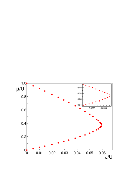
Figure 1: (Color online) Phase diagram of the first MI-SF lobe. Solid circles are numerical data, with error bars shown but barely visible. The inset is a blow up of the region close to the tip. Dashed lines represent the critical region as calculated from finite size scaling.

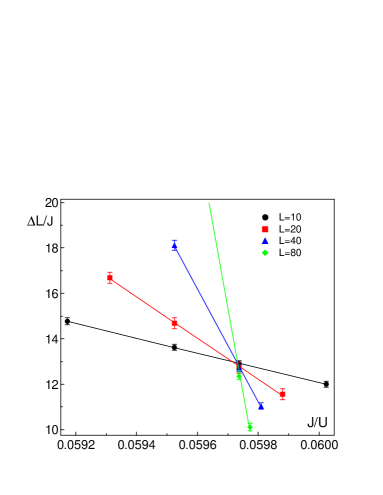
Figure 2: (Color online) Finite size scaling of the energy gap at the tip of the lobe. Lines represent linear fits used to extract the critical point. The critical point can be directly read from the intersection of the curves: $(J/U)_{c}=0.05974(3)$.

We now turn to the presentation of our results. The procedure used to determine the ground state phase diagram and extract effective masses of particle and hole excitations from the Green function was discussed in details in Ref. BH_3D . In Fig. 1 we present results for the ground state phase diagram corresponding to unity filling. The inset shows the region around the tip. Circles represent the simulation data while dash lines are obtained from the finite size scaling analysis. Simulations were done for linear system sizes $L=10,\;20,\;40,\;80$. We do not see any significant size effect up to $J/U\sim 0.057$. In order to extract the position of the critical point at the tip of the lobe and determine the extension of the critical region, the standard finite size scaling argument was used (see Ref. BH_3D ), with the critical exponent for the correlation length $\nu=0.6715$. The finite size scaling of the energy gap is presented in Fig. 2. One can directly read the position of the critical point from the intersection of the curves:

$$(J/U)_{c}=0.05974(3)\;\;\;\;(n=1).$$ (3)

Equation (3) and Fig. 1 constitute the most precise quantum Monte Carlo simulation for the Hamiltonian 1 which is in perfect agreement with the result of Ref. Monien , where the authors carried out a strong coupling expansion up to 13-th order. Note that the critical region in Fig. 1 is resolved with accuracy $\ll J$, i.e. for gaps $\Delta<J$, which is crucial for studies of the emerging relativistic physics at the lobe tip.
In Fig. 3 we plot effective masses for particle (circles) and hole (squares) excitations. Dispersion relations were fitted by a parabola, with the exception for $J/U=0.059$ where we used a relativistic dispersion relation. Close to the tip of the diagram, the action is isotropic in space and imaginary time, giving rise to a relativistic behavior Fisher . In the limit $J/U\rightarrow 0$, where one can calculate effective masses perturbatively, our data converge to the analytical result (dashed lines). To the first order, the perturbative expansions are given by (we set the lattice pariod and Planck’s constant equal to unity):

$$Jm_{+}=0.25-2J/U,\;\;\;\;\;Jm_{-}=0.5-8J/U$$ (4)

for particle and hole excitations respectively. On approach to the critical point, instead, data for particle and hole excitations are merging together, in agreement with the emergent particle-hole symmetry in the critical region. From the fit done at $J/U=0.059$ using the relativistic dispersion relation, we extract the value of the sound velocity $c/J=4.8\pm 0.2$ and effective mass $m_{*}=0.015\pm 0.0015$. We would like to point out that effective masses can also be extracted using the method of Ref. Monien , although we did not find any calculation in the literature.

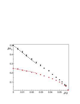
Figure 3: (Color online) Effective mass for particle (circles) and hole (squares) excitations as a function of $J/U$. The exact results at $J/U=0$ are $m_{+}=0.25/J$ and $m_{-}=0.5/J$. By dashed lines we show the lowest order in $J/U$ correction to the effective masses. Close to the critical point the two curves overlap, directly demonstrating the emergence of the particle-hole symmetry. At $J/U=0.059$, the sound velocity is $c/J=4.8\pm 0.2$.

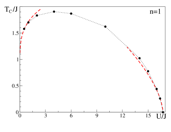
Figure 4: (Color online) Finite-temperature phase diagram at filling factor $n=1$. Solid circles are simulation results (the dotted line is to guide an eye), error bars are plotted. Dashed lines are analytical results for the weakly interacting gas [see Eq. (5)] and for the strongly interacting gas close $(J/U)_{c}$.

In Fig. 4 we show the phase diagram for the SF-normal transition at integer filling factor $n=1$. The transition is of Berezinskii-Kosterlitz-Thouless type KT . The critical temperatures were found from extrapolation to infinite system size of the standard finite size scaling for the Kosterlitz-Thouless transition (see e.g. Ref. KT_scaling ). In the figure, circles are numerical results and dashed lines are analytical expressions in the two limiting cases. In the weakly interacting regime the critical temperature is given by:

$$T_{c}=\frac{2\pi n}{m\ln(\xi/mU)},$$ (5)

where $n$ is the density ($n=1$ in this case), $m$ is the mass ($m=1/2J$ in the lattice), and $\xi$ is a dimensionless parameter which was found numerically in Ref. KT_scaling to be $\xi=380\pm 3$. On the approach of the critical point, instead, one can use the following scaling argument. Close to the critical point the superfluid density is $\rho_{s}(T=0)\sim\xi^{-1}\sim t^{\nu}$, where $t=(U/J-(U/J)_{c})$. Under the assumption $\rho_{s}(T=0)\sim\rho(T_{c})$, which should hold for low enough critical temperatures, i.e. close to the critical point $(U/J)_{c}$, one concludes that $T_{c}\sim\rho(T_{c})\sim t^{\nu}$. The dashed line in the plot is a fit done using the function $f(x)=At^{\nu}$, where A=0.49(2) is a fitting parameter. On both sides, numerical results clearly converge to the analytical expressions.
Many interesting phenomena happening at zero or nearly zero temperature have not been observed yet. This is because, so far, it has been a challenge for experimentalists to reach low enough temperatures. In order to overcome this challenge, one can exploit the inhomogeneity of the entropy distribution of the harmonically and optically trapped gas. The idea has been originally proposed in Ref. cooling_Cirac1 and cooling_Cirac2 , where the authors suggest several cooling protocols. Some of the protocols make use of the filtering scheme of Ref. filtering , others require spin dependent lattices. In all the protocols the main idea is to relocate the entropy by removing a small fraction of the particles carrying almost all the entropy. Recently it has also been suggested a cooling protocol based on coupling entropic particles with a system at lower temperature (i.e. a “refridgerator”) cooling_Ho . Having in mind a setup, similar to the one described in Ref. cooling_Cirac1 and cooling_Cirac2 , we would like to suggest a simple and efficient cooling protocol which does not require coupling to a refridgerator or exciting particles to a different internal energy level. Consider a system with $U\gg|\mu_{i_{0}}-\mu_{i=0}|,J,T$ and $|\mu_{i}-\mu_{i+1}|\gg J$, where $\mu_{i}$ is given by Eq. (2), $i=0$ is at the potential minimum while $i\sim i_{0}$ corresponds to the boundary of the system. The condition $U\gg|\mu_{i_{0}}-\mu_{i=0}|,J$ means that the groundstate density is essentially uniform. The condition $U\gg T$ guaranties that the entropy is located in a thin peripheral region of the system. In view of the condition $|\mu_{i}-\mu_{i+1}|\gg J$, the elementary excitations of the system are single-site (localized) particles and holes obeying Fermi statistics (in the real space) cooling_Cirac1 .

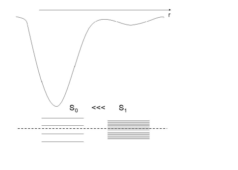
Figure 5: Sketch of the proposed cooling protocol. On top, a shallow and a deep trap are superimposed. At the bottom, the corresponding densities of states are sketched. The dashed line represents the Fermi level. Adiabatically displacing the shallow trap results in displacing entropic particles with consequent dramatic decrease of entropy per particle inside the deep trap.

Take two superimposed traps, a very steep one and a very shallow one. The density of energy levels of the shallow trap is very high as compared to that of the steep one. The shallow trap thus carries most of the entropy. Adiabatically displacing the shallow trap would then result in displacing “entropic” particles and ultimately separating them from the particles of the steep trap. Academically speaking, the very last stage of this process cannot be adiabatic in view of the exponentially suppressed tunnelling between two traps. However, this non-adiabaticity simply means that the two systems become independent, so that the (now dramatically decreased) entropy of the steep trap has nothing to do any longer with the state of the particles in the shallow trap. The procedure is sketched in Fig. 5. For better results, one can perform a number of cooling cycles consisting of the above-described entropy relocation procedure followed by adiabatically increasing (and subsequent decreasing) the $J/U$ ratio in order to lift the localization constraint preventing redistribution of tiny fraction of remanent particle and hole excitations in the bulk towards the perimeter. Another possibility for entropy relocation consists of progressively lowering the confinement below the Fermi level in order to evaporate the entropic particles from the system.
In conclusion, we have presented numerical results for the single component Bose-Hubbard model. We have confirmed previous calculations Monien for the critical point at the tip of the $n=1$ lobe and presented results for the effective masses for particle and hole excitations. We have determined the critical temperature for the SF-normal transition for the unity filling case. These benchmark calculations provide a robust test for the bosonic optical lattice emulator.
We are grateful to Tin-Lun Ho for useful discussions. This work has been supported by the DARPA OLE program.

References

- (1) N. Elstner, and H. Monien, Phys. Rev. B 59, 184 (1999).
- (2) M. Greiner, O. Mandel, T. Esslinger, T.W. Hansch, and I. Bloch, Nature 415, 39 (2002).
- (3) J. K. Chin, D. E. Miller, Y. Liu, C. Stan, W. Setiawan, C. Sanner, K. Xu, and W. Ketterle, Nature 443, 961 (2006).
- (4) M. Lewenstein, A. Sanpera, V. Ahufinger, B. Damski, A. Sen(De), and U. Sen, Advances in Physics 56, 243 (2007).
- (5) http://physics.harvard.edu/ greiner/newexp.html
- (6) A. B. Kuklov, and B. V. Svistunov, Phys. Rev. Lett. 90, 100401 (2003).
- (7) L. M. Duan, E. Demler, and M. D. Lukin, Phys. Rev. Lett. 91, 090402 (2003).
- (8) E. Altman, W Hofstetter, E. Demler, and M. D. Lukin, New J. Phys. 5, 113 (2003).
- (9) M. Greiner, I. Bloch, T. W. Hsnsch and T. Esslinger, Phys. Rev. A 63, 031401(R) (2001).
- (10) M. P. A. Fisher, P. B. Weichman, G. Grinstein, and D. S. Fisher, Phys. Rev. B 40, 546 (1989).
- (11) N. V. Prokof’ev, B. V. Svistunov, and I. S. Tupitsyn, Phys. Lett. A 238, 253 (1998); Sov. Phys. JETP 87, 310 (1998).
- (12) L. Pollet, K. Van Houcke, C. Kollath, and M. Troyer, in progress.
- (13) B. Capogrosso-Sansone, N. V. Prokof’ev, and B. V. Svistunov, Phys. Rev. B 75, 134302 (2007).
- (14) J. M. Kosterlitz, and D. J. Thouless, J.Phys. C 6, 1181 (1973).
- (15) N. Prokof’ev, O. Ruebenacker, and B. Svistunov, Phys. Rev. Lett. 87, 270402 (2001).
- (16) M. Popp, J.-J. Garcia-Ripoll, K. G. Vollbrecht, and J. I. Cirac, Phys. Rev. A 74, 013622 (2006).
- (17) M. Popp, J.-J. Garcia-Ripoll, K. G. H. Vollbrecht, and J. I. Cirac, New J. Phys. 8, 164 (2006).
- (18) P. Rabl, A. J. Daley, P. O. Fedichev, J. I. Cirac, and P. Zoller, Phys. Rev. Lett. 91, 110403(2003).
- (19) T.-L. Ho, and Q. Zhou, private communication.