Chaotic quantum dots with strongly correlated electrons.

Abstract

Quantum dots pose a problem where one must confront three obstacles: randomness, interactions and finite size. Yet it is this confluence that allows one to make some theoretical advances by invoking three theoretical tools: Random Matrix theory (RMT), the Renormalization Group (RG) and the $1/N$ expansion. Here the reader is introduced to these techniques and shown how they may be combined to answer a set of questions pertaining to quantum dots.
PACS 73.21, 71.10Ay

I INTRODUCTION

This colloquium is based on a lecture entitled ”Dots for Dummies” I have frequently given. The title was chosen, not to offend, but to keep experts in the audience from hijacking the lecture with minutiae while the intended goal was to introduce certain problems involving quantum dots to a broad audience not necessarily working in this subfield. The present article attempts to do the same for the general readership of this journal. To follow this colloquium you must be familiar with the rudiments of second quantization and Feynman diagrams.

The emphasis of this article is idiosyncratic. I am partial to what I know best and like to talk about most: a frankly pedagogical tour of several useful techniques and their applications to this problem. There is not a comparable emphasis on phenomenology, for which I will direct you to other excellent sources.

So let us begin by asking ”What are some of the questions in the world of quantum dots, what are some of the tools brought to bear in addressing them, and what are some of the answers?”

For our purposes, the dot is an island of size $L$ (in the nanoscale ) within which electrons are restricted to live.

If the dot is very small and the level spacing large (compared to other scales like temperature and interaction strength) we may be interested in just a few quantum states of the dot. For example if the dot is essentially a two-state system, one may study it with the intention of using it as a qubit in quantum computation. Here one needs to understand in detail the level structure of a particular dot so we can manipulate (program) it in a controlled way.

The focus here is on large dots with a very fine level spacing. These dots are closer to the bulk system of interacting fermions in that a large number of energy levels are in play. However the finite size and finite level spacing are essential features. These dots are very much like nuclei- finite systems of interacting fermions- with the main difference that the confining potential is externally imposed and not internally generated. The hard-wall boundary of the dot is assumed to be sufficiently irregular so that classical motion is chaotic at and around the Fermi energy. The dot is otherwise dirt-free and motion within is ballistic. The system is assumed to be quantum-coherent across the length of the dot.

Figure 1: A typical situation where leads bring in electrons which tunnel into and out of dot (opposite to the current shown by arrows). A gate voltage $V_{g}$ is the control parameter and $V$ is the vanishingly small source-drain voltage difference.

The dot is juxtaposed with leads that act as source and drain for electrons. Electrons are allowed to tunnel in and out of the dot. A gate voltage $V_{g}$ allows one to vary the dot energy relative to the Fermi energy of electrons in the leads as in Figure (1). A tiny voltage $V$ is applied between the source and drain to drive the current, and the conductance $G=I/V$ (in the limit of vanishing $I$ and $V$) is measured as a function of the gate voltage $V_{g}$ sketched in Fig (2).

Figure 2: A caricature of conductance $G$ versus gate voltage $V_{g}$. The peaks have varying heights, widths and spacings.

The theoretical challenge is to describe the observed series of peak positions and peak heights Guhr, Muller-Groeling and Weidenmuller (1998); Merlin (2000); Alhassid (2000); Aleiner et al. (2002); Jalabert, Stone and Alhassid (1992); Chang et al. (1996); Folk et al. (1996). These are decided by the shape of the empty dot, coupling to the leads, the number of electrons in it and the interactions between them. Now, no one disputes that given enough such information, every peak may be described in greatest detail since the underlying laws (nonrelativistic quantum mechanics and the Coulomb interaction) are thoroughly understood. However this is not the goal here. The goal is more akin to that set by Wigner in describing excited states of nuclei. A nucleus, like a dot, is a finite many-body system with strong interactions between its constituents. Wigner argued that while one could (in principle) describe the specific levels of a particular nucleus with its incredibly complicated Hamiltonian, it would more interesting to describe statistical properties of the spectrum. More specifically he suggested the following program. Consider a mathematical ensemble of Hamiltonians which have the same symmetries as the nuclear Hamiltonian (say, being real and hermitian) and have the same average level spacing. Calculate the statistics of level spacings in this ensemble. Compare this to the actual levels by averaging over members of the physical ensemble.

Note the difference with Statistical Mechanics, as emphasized by Guhr et al Guhr, Muller-Groeling and Weidenmuller (1998). There we consider an ensemble of systems with the same Hamiltonian but different initial conditions, while here we consider an ensemble of Hamiltonians with the same symmetry properties as the given nuclear Hamiltonian.

In the case of dots, the members of the physical ensemble contain dots with the same density of states. One can generate members of the ensemble by varying the number of electrons in one dot (which probes different energy regimes) or by manufacturing many similar dots of the same area. If dots of different sizes are used, one can rescale their energies so that the mean spacing is the same. The mathematical ensemble consists of Hamiltonians of the same symmetry class (e.g., real) and same average level spacing. In cases where there is a magnetic field (and the ensemble contains complex unitary Hamiltonians) one can also vary the field to move around the ensemble. (A minimum change in field may be needed to generate an independent member.)

Here are two kinds of questions one could ask:

• If I measure $\Delta$, the difference in gate voltage between successive peaks, what will be the probability distribution $P(\Delta)$?

• If I measure $G$, the maximum of each conductance peak, what will be the probability distribution $P(G)$?

There are of course other issues that we could discuss, but will not, such as the width of each peak as a function of temperature or spin content.

To get a feeling for the results, let us see how we would go about explaining the data, armed with just the theory of non-interacting electrons (whose spin will be initially ignored.)

To this end let us consider a particular dot of some particular shape. We would naturally begin by solving the single-particle Schrödinger equation

$$H_{0}\phi_{{\alpha}}({\mathbf{r}})={\varepsilon}_{{\alpha}}\phi_{{\alpha}}({\mathbf{r}})$$ (1)

with $\phi_{{\alpha}}({\mathbf{r}})=0$ at the boundary. This would have to be done on a computer for a generic dot. Imagine that we have all the wave functions $\phi_{{\alpha}}$ and energies ${\varepsilon}_{{\alpha}}$. Let $\delta_{i}={\varepsilon}_{i+1}-{\varepsilon}_{i}$ be the spacing between levels $i$ and $i+1$ and let $\delta$ stand for a generic one, as well as the average level spacing (which is the inverse density of states).

In the non-interacting theory, it is easy to see that at a randomly chosen value of gate voltage $V_{g}$, there will be no conduction. This is because the Fermi energy of the electrons in the lead will typically lie between occupied and empty levels in the dot, so that transmission by the occupied levels is forbidden by the Pauli principle and transmission by the empty levels is forbidden by energy conservation. However, when the Fermi energy of the leads equals an energy level of the dot there will be transmission. Note that during transmission the dot has the same energy with N or N+1 electrons. This feature survives even when interactions are included.

In this free-particle model, $\Delta_{i,i+1}$, the difference in the gate voltage $V_{g}$ between peak $i+1$ and peak $i$ times $-e$, the charge of the electron, will equal $\delta_{i,i+1}={\varepsilon}_{i+1}-{\varepsilon}_{i}$, the difference in energy between the level that was responsible for peak $i+1$ and the one that was responsible for peak $i$. It follows that (suppressing the constant $-e$)

$$P(\Delta)=P(\delta).$$ (2)

In other words, the distribution of spacings in $V_{g}$ between successive peaks is the same as the distribution of level spacings in the dot. Consequently, to obtain the statistical distribution $P(\Delta)$ theoretically, we need to solve for a large number of energy levels in one particular dot, record the spacings $\delta$, and repeat within the ensemble, which means here other dots with similar density of states but arbitrary shape. (In order to fold in the results from many dots and many energy ranges, it will be necessary to rescale energies so that $\delta$, the average level spacing, is fixed at some value.)

As for the height of any conductance peak, it will be given by the product of the probabilities for hopping on to the dot at the left lead $L$, and hopping off on the right lead $R$. These are determined $\phi_{{\alpha}}(L/R)$, the value near the leads of the wave function $\phi_{{\alpha}}$ corresponding to the state which is responsible for the transmission. One could collect the statistics of these as well, from our numerical solutions to Eqn. (1).

Now it turns out we can spare ourselves a lot of trouble in obtaining these probability distributions $P(\delta)$ and $P(G)$ by appealing to Random Matrix Theory or RMT, provided certain condition apply. So we begin with a crash course on RMT.

The first step is to acquaint ourselves with $E_{T}=\hbar v_{F}/L$, the Thouless energy, where $v_{F}$ is the Fermi velocity. Evidently $E_{T}$ stands for the uncertainty in energy of an electron that traverses the dot ballistically at the Fermi velocity in a time $\tau=L/v_{F}$. Thus if the dot is connected to big fat leads,

$$g\simeq{E_{T}\over\delta}$$ (3)

single particle levels in this energy window will each contribute a maximum of $e^{2}/h$ to conductance $G$. Thus in this case of a dot connected strongly to leads, $g$ will be the dimensional conductance, i.e., $G$ measured in units of the quantum of conductance $e^{2}/h$. .

While this is one way to introduce $E_{T}$, you could object that in the experiments we consider the leads are weakly coupled to the dot and the levels are sharp. You would be right, and it turns out we are interested in $E_{T}$ for the following different reason.

If the dot has a generic shape with no conserved quantities except for energy, and the classical dynamics at the Fermi energy is chaotic, the statistics of energy levels lying within a band of width $E_{T}$ and of the corresponding wave functions, are determined by RMTMehta (1991), given just general features like the average level spacing $\delta$ and symmetries of the Hamiltonian. This is like saying that the statistical properties of an isolated box of gas are determined by just gross features like volume, number of particles and energy. Such a statistical approach to the energy levels of very complicated systems was first taken by Wigner in the case of nuclei, which are once again finite systems made up of a large number of particles subject to strong interactions that defy any direct treatment. Notice that to use RMT you just need to know the symmetry class (real or complex matrix elements etc.) but no further details including even the spatial dimensionality of the problem.

The first RMT prediction is that $P(\delta)$, the distribution of exact energy level differences $\varepsilon_{i+1}-{\varepsilon}_{i}$ (for states lying with a band of width $E_{T}$), will be indistinguishable from that of an ensemble of random matrices of the same symmetry class, which in our problem, consists of all real hermitian matrices with the same $\delta$, the average level spacing. (For a dot in a magnetic field, where time-reversal symmetry is broken, the ensemble will consist of complex hermitian matrices.)

In other words, the results one person gets by painstakingly solving for the spectrum of an ensemble of dots and compiling the level statistics is same as that compiled by another person who picks real hermitian Hamiltonians out of a hat, diagonalizes them and plots their spacing distribution! Furthermore this universal distribution is known in analytic form as soon as we provide $\delta$.

So, history repeats itself: when things get really bad, (the dynamics goes from integrable to chaotic) they become good again because statistical methods become applicable.

The second RMT result bears on wave functions. A common quantity of interest is the ensemble average (denoted by $\langle\cdots\rangle$) of products of wave functions such as

$$\langle\phi_{{\alpha}}^{*}({\mathbf{r}})\phi_{\beta}({\mathbf{r}}^{\prime})\rangle$$ (4)

defined as follows. Pick one realization of the dot and number the states by energy, with ${\alpha}$ and $\beta$ being two such numerical labels. Pick two points ${\mathbf{r}}$ and ${\mathbf{r}}^{\prime}$ inside the dot. Find $\phi_{{\alpha}}^{*}({\mathbf{r}})\phi_{\beta}({\mathbf{r}}^{\prime})$. Now change the dot smoothly, staying within the ensemble. Since there is no level crossing in a chaotic dot, the labels ${\alpha}$ and $\beta$ retain their integrity. Now recompute $\phi_{{\alpha}}^{*}({\mathbf{r}})\phi_{\beta}({\mathbf{r}}^{\prime})$. Find the average of such terms over the entire ensemble. This is what Eq. (4) means. Such correlations are of use in computing peak-height distributions Jalabert, Stone and Alhassid (1992).

In our problem we need the correlation of wave functions in momentum space rather than coordinate space and we shall use them to deal with electron-electron interactions rather than to calculate $P(G)$.

Figure 3: The Wheel-of-fortune states within a band of energy $E_{T}$ concentric with the Fermi circle. There are roughly $g$ such states of mean momenta ${\mathbf{k}}$ centered on $g$ equally spaced points on the Fermi circle. The WOF states are obtained by chopping off plane waves of the desired mean momentum at the edges of the dot. These states are very nearly orthonormal.

Let us begin by modifying the definition of ”momentum space” as appropriate to the dot.

Consider a circular Fermi sea in ${\mathbf{k}}$ space and a concentric annulus of width $E_{T}$ in energy. In the bulk, this region contains an infinite number of ${\mathbf{k}}$ states. If we now go to the dot of size $L$, the best we can do vis-a-vis momentum is wave packets centered at some ${\mathbf{k}}$ and of width $1/L$ in both directions. It is readily verified that we can form $g$ such ”Wheel-of-fortune” (WOF) states (as in Figure 3)) within this annulus Murthy, Shankar and Mathur (2005). Suppose we expand the $g$ exact eigenstates (labeled by ${\alpha}$) of a dot within the Thouless band in this WOF basis (labeled by ${\mathbf{k}}$) via the functions $\phi_{\alpha}({\mathbf{k}})$ as follows

$$|{\alpha}\rangle=\sum_{{\mathbf{k}}}\phi_{\alpha}({\mathbf{k}})|{\mathbf{k}}\rangle.$$ (5)

Then a typical RMT result invoked here is that as $g\to\infty$

$$\left<\phi_{\alpha}^{*}({\mathbf{k}})\phi_{\beta}({\mathbf{k}}^{\prime})\right>={\delta_{{\mathbf{k}}{\mathbf{k}}^{\prime}}\delta_{\alpha\beta}\over g}+{\cal O}({1\over g^{2}})$$ (6)

where the $<\cdots>$ denote describe an average over an ensemble of similar dots.

Note that Eqn. (6) is the minimal correlation we must have: in each sample, $\alpha$ and ${\mathbf{k}}$ label two orthonormal bases, so that if we set ${\mathbf{k}}={\mathbf{k}}^{\prime}$ and sum over ${\mathbf{k}}$ we must get $\delta_{\alpha\beta}$, sample by sample and hence on average as well. (The same goes for setting $\alpha=\beta$ and summing over them to get $\delta_{{\mathbf{k}}{\mathbf{k}}^{\prime}}$.) Similar correlators exist for products of four wave functions and these have the form of Wick’s theorem.

Unlike the result on level spacings, which can be demonstrated analytically, this one on wave functions is an assumption we will make. A reader armed with the requisite determination and computing power is invited to confirm or contradict this assumption. All we can say is that several consequences of this assumption have been verified in our numerical work Murthy et al. (2004).

Before proceeding let me address a common question. Is there any reason to believe that the $g$ exact eigenstates within $E_{T}$ can be expanded in terms of the $g$ WOF states? We Murthy, Shankar and Mathur (2005) have verified the following in a numerical study of a ”billiard”, or dot. First we manufactured the $g$ states of mean momentum ${\mathbf{k}}$ by choosing $g$ equally spaced points on the Fermi circle and then chopping off the plane waves of these momenta at the edges of the billiard. (We chose $g=37$ in our study.) Then we verified that these wavefunctions were orthonormal to an excellent accuracy. Next we asked how good a basis these functions formed for expanding the $\alpha$ states within $E_{T}$. We found the exact eigenstate at the middle of the Thouless band, i.e, at the Fermi energy, retained more than 99.9% of its norm upon projection to the WOF basis. As we left the center of the band the overlap decreased and dropped to around 50% at the edges. Thus our results get more reliable as we go deeper into the Thouless band centered at the Fermi energy.

Let us turn to the data on $P(\Delta)$, the distribution of spacings in $V_{g}$ between peaks. In the noninteracting case we saw that $P(\Delta)=P(\delta)$, and then we saw that $P(\delta)$ was given by RMT.

So let us test the RMT results for level spacings $P(\delta)$, against $P(\Delta)$, the measured distribution of spacings in $V_{g}$ between successive peaks. These will match only if the assumptions of non-interacting electrons is correct.

The test fails. It is found that the peak spacings are an order of magnitude larger than level spacings in the dot. The reason is of course electron-electron interactions. Even if we ignore the full quantum mechanical treatment of interactions, we need to acknowledge the classical fact that when we add an electron to a dot, it experiences Coulomb repulsion for the other occupants. Thus the energy cost of adding an electron is not just that of going to the next empty level, it is the additional repulsive energy. This capacitive charging energy is proportional to $N^{2}$ and we must add a term $u_{0}N^{2}$ to the second quantized Hamiltonian. By studying the data one can come up with a good fit to $u_{0}$.

However we can anticipate that this alone will not work in the presence of spin, even in the non-interacting case. With spin present, each single particle orbital can be doubly occupied. Thus adding an electron will (will not) cost us a single particle energy level difference if it brings the total occupancy to an odd (even) integer. Combined with the above mentioned charging energy, we expect the peak spacing to have a bi-modal distribution as N varies from odd to even.

This is however not seen. The reason is based on the exchange interaction. While it makes sense to put two electrons in each orbital if one is minimizing kinetic energy, this may be a bad idea in terms of potential energy: the electrons in any given orbital would have opposite spins and hence the Pauli principle would not keep them away from each other, thereby raising the Coulomb repulsion. To minimize the potential energy we must occupy each orbital once and place the electrons in the same spin state so that the Pauli principle can keep them apart in space. To let the system decide what is best we must give it an incentive for higher spins by adding a term $-JS^{2}$, where $S$ is the total spin.

Thus we are led to the following (second-quantized) ”Universal” Hamiltonian: Aleiner et al. (2002); Oreget al. (2001); Andreev and Kamenev (1998); Browuer, Oreg and Halperin (1999); Baranger, Ullmo and Glazman (2000); Kurland,Aleiner and Altshuler (2000)

$$H_{U}=\sum_{\alpha}\psi^{{\dagger}}_{\alpha}\psi_{\alpha}\varepsilon_{{\alpha}}+u_{0}N^{2}-J_{0}S^{2},$$ (7)

where $\psi_{{\alpha}}$ destroys an electron in a state ${\alpha}$. A third possible interaction term pertaining to superconducting fluctuations has been dropped on the grounds that it is unimportant for the dots in question.

Some proponents of the universal Hamiltonian give the following argument for why no other interactions need be considered. Suppose we take any other familiar interaction and transcribe it to the exact basis. Sums of products of random wavefunctions $\phi_{\alpha}$ will appear and lead to terms with wildly fluctuating phases. These terms can be shown to have zero ensemble average as $g\to\infty$. Since deviations from the zero average will be down by $1/g$ we can drop them at large $g$. By contrast the two terms kept (which commute with $H_{0}$) are free of oscillations and survive ensemble averaging.

While the success of $H_{U}$ in explaining a lot of data is unquestioned, the accompanying arguments are not persuasive. In particular, ensemble averages should be performed not on the Hamiltonian but on calculated observables. It is also not clear that a group of terms should be dropped because they are small, since they could ultimately prove important to physics at very low energies (low, even within the already tiny band of width $E_{T}$).

Now there is a tried and tested way for determining the relative importance of possible interactions in the low energy limit. It is the Renormalization Group (RG). Not only can it tell us how important any given interactions is in the low energy sector, if there are competing interactions, it can provide an unbiased answer in which they are all allowed to fight it out. (As explained in Shankar (1994), The Luttinger Liquid in $d=1$ is an example in which Superconductivity and Charge Density Wave formation compete and actually annul each other while in $d=2$ the latter wins at half-filling on a square lattice.)

It is therefore natural to ask if the RG applicable in this problem and if so what its verdict is.

II The Renormalization Group - the ten cent tour

In order not to leave behind readers unfamiliar with the RG the following lightening review is provided. Experts can skip to the next section.

II.1 What is the RG?

Imagine that you have some problem in the form of a partition function

$$Z(a,b) = \int dx\int dye^{-a(x^{2}+y^{2})}e^{-b(x+y)^{4}}$$ (8)

$$\equiv \int dx\int dye^{-S(x,y;a,b,..)}$$ (9)

where $a$ and $b$ (along with other such possible terms) are constant parameters and $S$ is called the action. (In classical statistical mechanics it would be called the energy.)

The parameters $b$, $c$ etc., are called couplings and the monomials they multiply are called interactions. The $x^{2}$ term is called the kinetic or free-field term, and $a$, the coefficient of the kinetic term, has no name and is usually set equal to ${1\over 2}$ by rescaling $x$.

The average of any $f(x,y)$ is given by

$$\langle f(x,y)\rangle={\int dx\int dyf(x,y)e^{-a(x^{2}+y^{2})}e^{-b(x+y)^{4}}\over\int dx\int dye^{-a(x^{2}+y^{2})}e^{-b(x+y)^{4}}}.$$ (10)

Suppose we are interested only in functions of just $x$. In this case

$$\langle f(x)\rangle = {\int dxf(x)\int dye^{-a(x^{2}+y^{2})-b(x+y)^{4}}\over\int dx\int dye^{-a(x^{2}+y^{2})-b(x+y)^{4}}}$$ (11)

$$\equiv {\int dxf(x)e^{-a^{\prime}x^{2}-b^{\prime}x^{4}+..}\over\int dxe^{-a^{\prime}x^{2}-b^{\prime}x^{4}+..}}$$

where

$$e^{-a^{\prime}x^{2}-b^{\prime}x^{4}..}=\int dye^{-a(x^{2}+y^{2})-b(x+y)^{4}}$$ (12)

defines the parameters $a^{\prime},b^{\prime}...$etc. In the general case we would like to define an effective action $S^{\prime}(x;a^{\prime},b^{\prime},c^{\prime}..)$ by

$$e^{-S^{\prime}(x;a^{\prime},b^{\prime},c^{\prime}..)}=\int dye^{-S(x,y;a,b,c,..)}$$ (13)

and the corresponding partition function

$$Z(a^{\prime},b^{\prime}...) = \int dxe^{-S^{\prime}(x;a^{\prime}b^{\prime}c^{\prime}..)}$$ (14)

which define the effective theory for $x$. These parameters $a^{\prime}$, $b^{\prime}$ etc., will reproduce exactly the same averages for $x$ as the original ones $a,b,c..$ did in the presence of $y$. This evolution of parameters with the elimination of uninteresting degrees of freedom, is called renormalization. It has nothing to do with infinities; you just saw it happen in a problem with just two variables.

Note that even though $y$ does not appear in the effective theory, its effect has been fully incorporated in the process of integrating it out to generate the renormalized parameters. We do not say ” We are not interested in $y$, so we will set it equal to zero everywhere it appears”, instead we said, ”What theory, involving just $x$, will give the same answers as the original theory that involved $x$ and $y$?”

The term ”Group” arises as follows. Let us say $y$ is a short hand for many variables as is always the case in real life. If we eliminate one of them, say $y_{1}$ which leads to the renormalization $(a,b,c,..)\to(a^{\prime},b^{\prime},c^{\prime}..)$ and then we eliminate $y_{2}$ so that now $(a^{\prime},b^{\prime},c^{\prime},..)\to(a",b",c"..)$ the net result is equivalent to a single renormalization process in which $(a,b,c,..)\to(a",b",c"..)$ under the elimination of $y_{1}$ and $y_{2}$. (The RG is not a real group since we cannot define a unique inverse.)

II.2 How is mode elimination actually done?

Notice that to get the effective theory we need to do a non-gaussian integral. This can only be done perturbatively. At the simplest Tree Level, we simply drop $y$ and find $b^{\prime}=b$.

In other words, at tree level, the effective action is found by simply setting the unwanted variables to zero in the original action.

At higher orders, we bring down the non-quadratic exponential and integrate in $y$ term by term and generate effective interactions for $x$.

Here is how it is done in our illustrative example.

$$e^{-S^{\prime}} = e^{-ax^{2}-bx^{4}}\int dye^{-ay^{2}}e^{-b(4xy^{3}+4x^{3}y+6x^{2}y^{2}+y^{4})}$$ (15)

$$= \!\!e^{-ax^{2}-bx^{4}}Z_{0}(a)\!{\int\!\!dye^{-ay^{2}}\!e^{-b(4xy^{3}+4x^{3}y+6x^{2}y^{2}+y^{4})}\over Z_{0}(a)}$$

$$= \!\!e^{-ax^{2}-bx^{4}}\!Z_{0}(a)\langle e^{-b(4xy^{3}+4x^{3}y+6x^{2}y^{2}+y^{4})}\rangle_{Z_{0}}$$

where we have multiplied and divided by $Z_{0}(a)$,

$$Z_{0}(a)=\int dye^{-ay^{2}}$$ (16)

the partition function for a Gaussian action $e^{-ay^{2}}$ and where

$$\langle e^{-b(4xy^{3}+4x^{3}y+6x^{2}y^{2}+y^{4})}\rangle_{Z_{0}}$$ (17)

stands for the average of the exponential with respect to the partition function $Z_{0}(a)$. Since $Z_{0}(a)$ is independent of $x$, we will simply ignore it in the effective action $S^{\prime}(x;a^{\prime},b^{\prime}..)$, without altering any absolute probability. As for Eq. (17) we invoke the result valid for averages over Gaussian actions:

$$\langle e^{-V}\rangle_{Z_{0}}=e^{-\langle V\rangle-{1\over 2}(\langle V^{2}\rangle-(\langle V\rangle)^{2}\rangle\ldots}.$$ (18)

This is called the cumulant expansion and we see that in our example where $V=b(4xy^{3}+4x^{3}y+6x^{2}y^{2}+y^{4})$, the exponent is a power series in $b$ for contributions to $S^{\prime}$.

To the leading order in $b$ we have

$$S^{\prime}(x;a^{\prime},b^{\prime}..) = ax^{2}+bx^{4}+\langle b(4xy^{3}+4x^{3}y+6x^{2}y^{2}+y^{4})\rangle$$ (19)

$$= ax^{2}+bx^{4}+6bx^{2}\langle y^{2}\rangle+\langle y^{4}\rangle$$

$$= ax^{2}+bx^{4}+6b{x^{2}\over 2a}+{3\over 4a^{2}}$$

because $\langle y\rangle=\langle y^{3}\rangle=0$, $\langle y^{2}\rangle={1\over 2a}$ and $\langle y^{4}\rangle={3\over 4a^{2}}$. Thus we have our first RG result for renormalization:

$$a^{\prime}=a+{3b\over a}$$ (20)

to leading order in $b$. Note that we do not care about $x$-independent constants like ${3\over 4a^{2}}$. For reader who know Feynman diagrams, the power series in $b$ can be identified with the Feynman graphical expansion for a $\phi^{4}$ theory (since we kept up to quartic terms in the action.) In the case of the actual $\phi^{4}$ field theory itself, when the momentum cut-off is reduced from ${\Lambda}$ to ${\Lambda}/s$ (where $s>1$), $x$ will denote low-momentum modes $0<k<{\Lambda}/s$ and $y$ the high-momentum modes ${\Lambda}/s<k<{\Lambda}$, and the loop integration will be over the range ${\Lambda}/s<k<{\Lambda}$.

II.3 Why do the RG?

Why do we do this? Because the ultimate effect of any coupling on the fate of $x$ (the variable we care about) is not so apparent when $y$ (the variable in which we have no direct interest) is around, but surfaces to the top only as we zero in on $x$. For example, we are going to consider a problem in which $x$ stands for many low-energy variables and $y$ for many high energy variables. As we integrate out high energy variables and zoom in on the low energy sector, an initially tiny coupling can grow in size, or an initially impressive one diminish into oblivion.

This notion can be made more precise as follows. Consider the gaussian model in which we have just $a\neq 0$. We have seen that this value does not change as $y$ is eliminated since $x$ and $y$ do not talk to each other. This is an example of a fixed point of the RG since the coupling that goes in comes out unchanged by elimination of unwanted variables. Now turn on new couplings or ”interactions” (corresponding to higher powers of $x$, $y$ etc.) with coefficients $b$, $c$ and so on. Let $a^{\prime}$, $b^{\prime}$ etc., be the new couplings after $y$ is eliminated. Let us in addition rescale $x$ so that $x^{2}$ has the same coefficient as before i.e., $a^{\prime}=a={1\over 2}\mbox{say}$. Any of the renormalized couplings (still called $b^{\prime},c^{\prime},..$), which are are bigger than the initial ones, $b,c,d..$, are called relevant while those that are smaller are called irrelevant. This is because in reality $y$ stands for many variables, and as they are eliminated one by one, the relevant coefficients will keep growing with each elimination and the irrelevant ones will keep shrinking and ultimately disappear. If a coupling neither grows not shrinks it is called marginal. Thus the RG will tell us which couplings really matter in the low energy limit which controls the nature of the ground state and its low lying excitations.

There is another excellent reason for using the RG, and that is to understand the phenomenon of universality in critical phenomena, an area I will not enter.

Later we will apply these methods to quantum dots. For the reader who may understandably get restless in the interim, here is a glimpse how we will use RG in the case of dots. First we will begin with all single-particle states in the Hilbert space of dot. Then we will zero in on states lying within a narrow band of states within an energy $E_{L}$ the Fermi energy $E_{F}$. (All one needs is that $E_{L}<<E_{F}$.) In other words, at this point the variables we called $x$ ($y$ ) are states lying inside (outside) this band. For the clean system in the bulk, the result of such a mode elimination is known Shankar (1994) to lead to the result that the system is described by an infinite number of Landau Fermi Liquid parameters $u_{m}$, where $m$ is an integer. This process will be discussed in abridged form. The Universal hamiltonian contains just the $u_{0}$ term. We would like RG to tell us if and when we can ignore all other $u_{m}$’s. To this end we will begin with a theory where only states within $E_{T}$ of $E_{F}$ are kept and the starting hamiltonian has all Landau interactions written in terms of the dot eigenfunctions $\phi_{\alpha}$. Then we will ask what happens to them as we eliminate states within $E_{T}$, getting even closer to $E_{F}$. To see what happens when we do this (and how we do this) you need to read on!

III The problem of interacting fermions

We will now apply RG to a system of nonrelativistic spinless fermions of mass $m$ and momentum ${\mathbf{K}}$ in two space dimensions. The single-particle Hamiltonian is

$$H={K^{2}\over 2m}-\mu$$ (21)

where the chemical potential $\mu$ is introduced to make sure we have a finite density of particles in the ground state: all levels within the Fermi surface, a circle defined by

$${K^{2}_{F}\over 2m}=\mu$$ (22)

are now occupied since occupying these levels lowers the ground-state energy.

In second-quantization we are thus starting with the Hamiltonian

$$H_{0}=\int d^{2}K{\psi^{{\dagger}}}({\mathbf{K}})\left({K^{2}-K_{F}^{2}\over 2m}\right)\psi({\mathbf{K}})$$ (23)

where $\psi^{{\dagger}}({\mathbf{K}})$ creates a fermion of momentum ${\mathbf{K}}$. Notice that this system has gapless excitations above the ground state. You can take an electron just below the Fermi surface and move it just above, and this costs as little energy as you please. Such a system will carry a dc current in response to a dc voltage. An important question one asks is if this will be true when interactions are turned on. For example the system could develop a gap and become an insulator. Or it could become a superconductor. How do we decide what the fermionic ground state and low energy excitations will be, short of solving the problem?

In the noninteracting limit the ground state is simple: it is a single Slater determinant (antisymmetrized wave function) with all momentum states below $K_{F}$ occupied. If we turn on say, quartic interactions, the new ground state will have pieces in which two fermions from below $K_{F}$ have been moved to two fermions above $K_{F}$ keeping the total momentum at zero. Each such piece will come with a numerator proportional to the interaction strength and an energy denominator equal to the cost of creating this particle-hole pair. Clearly fermions deep in the sea will not take part in this kind of process with any serious likelihood as long as the interactions to be added are weak. Likewise if states far above $K_{F}$ were removed no one would be the wiser. Thus the fate of the system is going to be decided by states near the Fermi energy. This is the great difference between this problem and the usual ones in relativistic field theory and statistical mechanics. Whereas in the latter examples low energy means small momentum, here it means small deviations from the Fermi surface. Whereas in these older problems we zero in on the origin in momentum space, here we zero in on a surface. The low energy region is shown in Figure 4.

We are now going to add interactions and see what they can do. This is going to involve further reduction of the cut-off. Here we join the discussion of Shankar (1994).

Let us begin then with a momentum band of width $\Lambda$ on either side of the Fermi surface. (In terms of energy, the band has a width $E_{L}$, where $L$ stands for Landau, for reasons that will follow. )

Figure 4: The low energy region for nonrelativistic fermions lies within the annulus concentric with the Fermi circle. It extends ${\Lambda}$ in momentum and $E_{L}$ in energy from the Fermi circle. In units where the Fermi velocity $v_{F}$ is chosen to be unity, the two are equal.

Let us first learn how to do RG for noninteracting fermions. To apply our methods we need to cast the problem in the form of a path integral. Following any number of sources, say Shankar (1994) if you want to one-stop shopping, we obtain the following expression for the partition function of free fermions:

$$Z_{0}=\int\left[d\psi d\overline{\psi}\right]e^{S_{0}}\\$$ (24)

where

$$S_{0}=\int d^{2}K\int_{-\infty}^{\infty}d\omega\overline{\psi}(\omega,{\mathbf{K}})\left(i\omega-{(K^{2}-K_{F}^{2})\over 2m}\right)\psi(\omega,{\mathbf{K}})$$ (25)

and

$$\left[d\psi d\overline{\psi}\right]=\prod_{\omega,{\mathbf{K}}}d\psi(\omega,{\mathbf{K}})d\overline{\psi}(\omega,{\mathbf{K}})$$ (26)

and $\psi$ and $\overline{\psi}$ are called Grassmann variables. They are really weird objects one gets to love after some familiarity. There are some rules for doing integrals over them. For now, I suggest you note only that (i) $\overline{\psi}(\omega,{\mathbf{K}})$ and $\psi(\omega,{\mathbf{K}})$ are defined for each $\omega$ and ${\mathbf{k}}$ in the annulus (ii) $Z$ is a product of Gaussian integrals, with the variables at each $(\omega,{\mathbf{K}})$ not coupled with those at another. The dedicated reader can learn more from Ref. Shankar (1994).

We now adapt this general expression to a thin annulus to obtain

$$Z_{0}=\int\left[d\psi d\overline{\psi}\right]e^{S_{0}}\\$$ (27)

where

$$S_{0}=\int_{0}^{2\pi}d\theta\int_{-\infty}^{\infty}d\omega\int_{-\Lambda}^{\Lambda}dk\overline{\psi}(i\omega-v_{F}\ k)\psi.$$ (28)

We have approximated as follows:

$${K^{2}-K_{F}^{2}\over 2m}\simeq{K_{F}\over m}\cdot k=v_{F}\ k$$ (29)

where $k-K-K_{F}$ and $v_{F}$ is the Fermi velocity, hereafter set equal to unity. Thus $\Lambda$ can be viewed as a momentum or energy cut-off $E_{L}$ measured from the Fermi circle. We have also replaced $KdK$ by $K_{F}dk$ and absorbed $K_{F}$ in $\psi$ and $\overline{\psi}$. It will be seen that neglecting $k$ in relation to $K_{F}$ is irrelevant in the technical sense.

Let us now perform mode elimination and reduce the cut-off by a factor $s$. Since this is a gaussian integral, mode elimination just leads to a multiplicative constant we are not interested in. So the result is just the same action as above, but with $|k|\leq\Lambda/s$. Consider the following additional transformations:

$$(\omega^{\prime},k^{\prime}) = s(\omega,k)$$ (30)

$$(\psi^{\prime}(\omega^{\prime},k^{\prime}),\overline{\psi}^{\prime}(\omega^{\prime},k^{\prime})) = \!\!s^{-3/2}\!\!\left(\!\psi\left({\omega^{\prime}\over s},\!{k^{\prime}\over s}\right),\overline{\psi}\!\left({\omega^{\prime}\over s}\!,{k^{\prime}\over s}\!\right)\right).$$

When you perform the highly recommended exercise of making this change of variables, you will find that the action and the phase space all return to their old values. So what? Recall that our plan is to evaluate the role of quartic interactions in low energy physics as we do mode elimination. Now what really matters is not the absolute size of the quartic term, but its size relative to the quadratic term. Keeping the quadratic term identical before and after the RG action makes the comparison easy: if the quartic coupling grows, it is relevant; if it decreases, it is irrelevant, and if it stays the same it is marginal.

Let us now turn on a generic four-Fermi interaction in path-integral form:

$$S_{4}=\int\overline{\psi}(4)\overline{\psi}(3)\psi(2)\psi(1)u(4,3,2,1)$$ (32)

where $\int$ is a shorthand:

$$\int\equiv\prod_{i=1}^{3}\int{d\theta_{i}}\int_{-\Lambda}^{\Lambda}dk_{i}\int_{-\infty}^{\infty}d\omega_{i}$$ (33)

At the tree level, we simply keep the modes within the new cut-off, rescale fields, frequencies and momenta , and read off the new coupling, a highly recommended exercise. We find

$$u^{\prime}(k^{\prime},\omega^{\prime},\theta)=u\left({k^{\prime}\over s},{\omega^{\prime}\over s},\theta\right).$$ (34)

This is the evolution of the coupling function. To deal with coupling constants with which we are more familiar, we expand the functions in a Taylor series (schematic)

$$u=u_{0}+ku_{1}+k^{2}u_{2}...$$ (35)

where $k$ stands for all the $k$’s and $\omega$’s and of course the $\theta$-s are fixed. An expansion of this kind is possible since couplings in the action are nonsingular in a problem with short range interactions. If we now make such an expansion and compare coefficients in Eqn. (34), we find that $u_{0}$ is marginal and the rest are irrelevant, as is any coupling of more than four fields. For example

$$u_{0}^{{}^{\prime}}=u_{0}\ \ \ u_{1}^{{}^{\prime}}={u_{1}\over s}\ \ \ u_{n}^{{}^{\prime}}={u_{n}\over s^{n}}$$ (36)

Suppose we start with some cut-off $\Lambda_{0}$ and an initial coupling, we shall call $u_{n}(0)$. Let us now reduce $\Lambda$ continuously as per $\Lambda=\Lambda_{0}e^{-t}\equiv\Lambda/s$ so that the change in $u_{n}$ is continuous in $t$. The relation $u_{n}^{{}^{\prime}}=u_{n}/s^{n}$, Eq. (36), can be written as $u_{n}(t)=u_{n}(0)e^{-nt}$,

Sometimes this result is rewritten in terms of the $\beta$-function;

$$\beta(t)={du_{n}(t)\over dt}=-nu_{n}(t)\ \ \ \ \mbox{ where $t=\ln s$.}$$ (37)

If you consider the $\phi^{4}_{4}$ scalar field theory in four dimensions you find again an equation like Eq.(35) with the difference that $k$ is measured from the origin and not the Fermi surface. Thus all we have left to worry about is one number $u_{0}$, the first term in the Taylor series about the origin, to which the low energy region collapses. Here the low energy manifold is a 2-sphere no matter how small $\Lambda$ is and $u_{0}$ will inevitably have dependence on the angles on the Fermi surface:

$$u_{0}=u(\theta_{1},\theta_{2},\theta_{3},\theta_{4})$$

Therefore in this theory we are going to get coupling functions and not a few coupling constants.

Let us analyze this function. Momentum conservation should allow us to eliminate one angle. Actually it allows us more because of the fact that these momenta do not come form the entire plane, but a very thin annulus near $K_{F}$. Look at Figure 5. Assuming that the cutoff has been reduced to the thickness of the circle in the figure, it is clear that if two points ${\mathbf{K}}_{1}$ and ${\mathbf{K}}_{2}$ are chosen from it to represent the incoming lines in a quartic coupling, the outgoing ones are forced to be equal to them (not in their sum, but individually) up to a permutation, which is irrelevant for spinless fermions. Thus we have in the end just one function of two angles, and by rotational invariance, their difference:

$$u(\theta_{1},\theta_{2},\theta_{1},\theta_{2})=F(\theta_{1}-\theta_{2})\equiv u(\theta).$$ (38)

About forty years ago Landau came to the very same conclusionLandau (1956), that a Fermi system at low energies would be described by one function defined on the Fermi surface. He did this without the benefit of the RG and for that reason, some of the leaps were hard to understand.

Figure 5: Kinematical reason why momenta are individually conserved up to a permutation.

Since $u$ is marginal at tree level, (gets neither big nor small as the RG process is iterated and modes are eliminated) we have to go to higher orders in perturbation theory to break the tie, to see if it ends up being relevant or irrelevant. The answer, given without proof, is that it remains marginal to all orders Shankar (1994). This is for strange kinematical reasons. A brief review of how the higher order calculation will be done will be given when we come to dots.

Often one writes

$$u(\theta)=\sum_{m}u_{m}\cos(m\theta)$$ (39)

where $u_{m}$ are the Landau parameters. The corresponding interaction is, in schematic form with radial integrals over $k$ suppressed,

$$H_{L}=\sum_{\theta,\theta^{\prime}}n(\theta)n(\theta^{\prime})u_{m}\cos\left(m(\theta-\theta^{\prime})\right)$$ (40)

where $n(\theta)$ is the number density at angle $\theta$ on the Fermi circle.

Note that if $u_{0}$ is the only non-vanishing Landau coupling, we get the $u_{0}N^{2}$ interaction of $H_{U}$. If we include spin, there are spin density-spin density interactions and $J_{0}$ corresponds to keeping just the zeroth harmonic. So $H_{U}$ amounts to keeping just the lowest harmonic in the Landau expansion.

We need to ask when and why $m>0$ terms can be ignored.

IV RG meets dots

The first crucial step towards this goal was taken by Murthy and Mathur Murthy and Mathur (2002). Their strategy was as follows.

• Step 1: Use the clean system RG described above to learn that at low energies the important interactions are the Landau interactions (of which $u_{0}$ and $J_{0}$ are a subset).

• Step 2: Start at the energy scale $E_{T}$ and switch to the exact basis states of the chaotic dot, writing the kinetic term and all the Landau terms in this basis. Run the RG by eliminating exact energy eigenstates within $E_{T}$. See what happens to all Landau terms, do they grow, fall or stay the same?

I will discuss some of the subtleties here, referring you to Murthy et al. (2004) for more details.

A common concern is to ask if we can ignore the walls of the dot and use momentum states at high energies. After all, momentum is not conserved in the dot and what meaning is there to using the Landau interaction written in the momentum basis? The point is this. Consider the collision of two particles in a box. As long as the collision takes place quickly (in terms of the time to cross the box) the incoming and outgoing particles can be labeled by momenta and this label will be useful (conserved) during the collision.

However this only brings us down to $E_{L}$, the energy below which Landau theory works. Although $E_{L}<<E_{F}$, it is still finite for an infinite system while $E_{T}\simeq 1/L$ is even smaller for large $L$. In this no man’s land between $E_{L}$ and $E_{T}$, the flow of couplings is intractable and landau parameters could have evolved from their bulk values. So what we are saying is this: the universal Hamiltonian has just two of the infinite Landau parameters ($u_{0},J_{0}$) in it. Let us put in the rest of them with any size, and see what their fate is under further mode elimination.

While this looks like a reasonable plan, it is not clear how it is going to be executed. There are at least two obvious problems. To understand them you must understand in more detail how the RG is done at the one loop level. To illustrate this we use the more familiar scalar theory in $d=4$ with the $u_{0}\phi^{4}$ interaction, where $u_{0}$, hereafter called just $u$, is marginal and momentum-independent. Suppose we want the scattering amplitude of four scalar particles. The answer will be given by a perturbation series, depicted in Fig. (6). The second term is an integral over the loop momentum $K$ that goes from $0\leq K\leq\Lambda$. The integrand is the product of the two propagators, which go as $1/K^{2}$ each at large $K$. (We have assumed the external momenta are all zero and neglected two other loop diagrams that behave the same way.) The left hand side corresponds to a physical process and cannot depend on the cut-off $\Lambda$. It follows $u$ must acquire $\Lambda$-dependence so as to make the right hand side $\Lambda$-independent. We can find $u({\Lambda})$ as follows. Suppose ${\Lambda}$ is reduced by $|d{\Lambda}|$. The loop will change by an amount equal to the integral in the region ${\Lambda}-|d{\Lambda}|<K<{\Lambda}$, which is now missing. This missing part must then come from the first term to keep the physical scattering amplitude fixed. A simple calculation shows that up to numerical factors

$$du=-u^{2}{|d{\Lambda}|\over{\Lambda}}$$ (41)

so that

$$\beta(t)={du\over dt}=-u^{2}.$$ (42)

In summary, the change in $u({\Lambda})$ is given by the loop terms with internal lines restricted to the modes being eliminated.

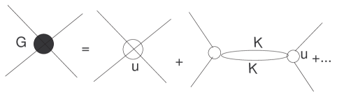
Figure 6: Schematic of scattering amplitude in $\phi^{4}$ theory. The solid dot is the full answer and the empty one is the coupling constant that goes in. The loop is the first of many that enter.

We run into the following problems if we try to do the mode elimination for the dot.

First, knowledge of the exact eigenfunctions is needed to even write down the Landau interaction (the analog of $u$ in the $\phi^{4}$ example) in the disordered basis:

$$V_{\alpha\beta\gamma\delta} = \sum\limits_{{\mathbf{k}}{\mathbf{k}}^{\prime}}u(\theta-\theta^{\prime})\left(\phi^{*}_{\alpha}({\mathbf{k}})\phi^{*}_{\beta}({\mathbf{k}}^{\prime})-\phi^{*}_{\alpha}({\mathbf{k}}^{\prime})\phi^{*}_{\beta}({\mathbf{k}})\right)$$ (43)

$$\times\left(\phi_{\gamma}({\mathbf{k}}^{\prime})\phi_{\delta}({\mathbf{k}})-\phi_{\gamma}({\mathbf{k}})\phi_{\delta}({\mathbf{k}}^{\prime})\right)$$

where ${\mathbf{k}}$ and ${\mathbf{k}}^{\prime}$ take $g$ possible values, ${\theta}$ and ${\theta}^{\prime}$ are the angles associated with ${\mathbf{k}}$ and ${\mathbf{k}}^{\prime}$ and the interaction has been antisymmetrized to mate with the four-Fermi operators $\psi^{{\dagger}}_{{\alpha}}\psi^{{\dagger}}_{{\beta}}\psi_{{\gamma}}\psi_{{\delta}}$.

Next, additional information is needed on energy levels to do the higher order (loop) calculation since the propagator for state ${\alpha}$ is $(i\omega-\varepsilon_{{\alpha}})^{-1}$. Remarkably it is possible to overcome ignorance of specific energy levels and wavefunctions. Here are some, but not all details of how this comes about.

First consider a specific realization. We want to reduce the cut-off by summing over some high energy-states ($y$’s). If we write down expression for the one loop flow, four-fold products of the unknown wave functions appear at each vertex. At the left vertex, two of these wave functions correspond to external lines, which are fixed (and below the new cut-off, i.e., these are the $x$ variables) while the other two correspond states to be eliminated and thus summed over. A similar thing happens at the right vertex. In addition there are the propagators for the two lines dependent on the single-particle energies.

Thus what we have here is a product of four wavefunctions and an energy denominator summed over states being eliminated. This sum will of course vary from dot to dot. Suppose we ignore this variation and replace the sum by its ensemble average. (The product of wavefunctions and the energy denominators can be averaged independently since to leading order in $1/g$, RMT does not couple them.) The entire average will then be just a function of just $g$ as in Eq. (4). But what about sample-to-sample variations? Here we invoke the nice result Murthy and Mathur (2002) that that deviations from the average are down by an extra power of $g$. Thus the flow is self-averaging, and every dot will have the same flow as $g\to\infty$.

Using such a device, these authors found the remarkable result that the renormalized $V_{\alpha\beta\gamma\delta}$ is itself equivalent to a Landau interaction but with renormalized values of $u_{m}$ flowing as per

$${du_{m}\over dt}=-u_{m}-cu_{m}^{2}\ \ \ \ m\neq 0$$ (44)

where $c$ is independent of $m$ and of order unity.

Note that $u_{0}$ does not flow and that just as in the BCS flow of the clean system Shankar (1994), different $m$’s do not mix to this order. If spin were included $J_{0}$ wouldn’t flow either. This lack of flow is due to the fact these coefficients multiply operators that commute with $H_{0}$, the non-interacting part of the Hamiltonian, and therefore have no quantum fluctuations.

The flow (for $m\neq 0$) implies that all positive $u_{m}$’s flow to zero, as do negative ones with $u_{m}>u^{*}$, the fixed point of the flow. Thus all points to the right of $u^{*}$ flow to $H_{U}$, as shown in Fig. 7. If a modest amount of $u_{m},m>0$ of either sign is turned on at the beginning (when ${\Lambda}=E_{T}$), it will renormalize to zero as we go down in energy. On the other hand if we begin to the left of $u^{*}$, we run off to large negative values.

The universal Hamiltonian is thus an RG fixed point with a domain of attraction of order unity. To me this is the most satisfactory explanation of its success.

Figure 7: The flow of the coupling $u_{m}$ for any $m\neq 0$. The origin of this flow is the universal Hamiltonian where every $u_{m}=0$ except $u_{0}$ which can have any value. All points to the right of $u^{*}$ flow to this. We ask what happens if we begin to the left.

V The $1/N$ approximation

So far we have used the RG to understand the low energy behavior of the quantum dot. We found that if we begin our analysis with states within $E_{T}$ of the Fermi energy $E_{F}$ and all possible Landau interactions $u_{m}$, and slowly reduce the energy cut-off, we end up with the universal Hamiltonian as the low energy fixed point for all positive $u_{m}$’s and negative $u_{m}$’s that are are not more negative than some critical value $u_{m}^{*}$. From this knowledge at very low energies we can conclude in particular that the ground state (lowest of all energies!) is determined by $H_{U}$ for $u_{m}>u_{m}^{*}$ and that at $u_{m}=u_{m}^{*}$ the system undergoes a second order phase transition, for that is what a zero of the beta function or fixed point signifies. The RG does not tell us much about the nature of the new phase, other than that it will be dominated by the $u_{m}$ that runs off to strong coupling.

While this is nice, there is clearly room for improvement. In particular, if the theory could be solved exactly, we would know even more. We would know if the phase transition at $u_{m}$ of order unity, found in the perturbative, one-loop calculation, really does occur. We would also know to what state the system is driven after the transition. In other words, if we can solve a problem exactly, we do not need the RG. We could, after obtaining the solution with some cut-off, easily ask how the coupling is to be modified if the cut-off is then reduced. We would do this by computing a physical quantity $P(u(\Lambda),\Lambda)$ as a function of the input cut-off $\Lambda$ and input coupling $u(\Lambda)$ and then set $dP/d\Lambda=0$ to find $du/d\Lambda$. This would be the exact beta function that one could compare to any perturbative result.

It turns out we can do all this in our problem of dots. Now, any controlled calculation is based on some small quantity. If the small quantity vanishes the controlled calculation gives exact results. The most common example is the coupling constant itself, and the exact solution that emerges in the limit of zero coupling is a free theory. However, there are other cases exhibiting nontrivial behavior, where the coupling is not small but something else is. For our dots the small parameter turns to be $1/g$ and the exact solution emerges in the limit $g\to\infty$ as Murthy and I Murthy and Shankar (2003) found. Note that the limit $g\to\infty$ corresponds to the limit of infinite dot size. (Unfortunately this does not mean we understand bulk physics, since in this large dot the Thouless band, over which we have control using RMT, shrinks to zero as $1/L$.) What we assume is that what happens in this infinite dot will seen also in large but finite dots, just as one assumes that genuine phase transitions, which are allowed only in infinite systems will be well mimicked in large but finite systems. We could show that in this limit there is indeed a transition at a negative coupling of order unity and that to the left of it is a symmetry-broken phase which can be analyzed in some detail.

We showed that one did not have to rely on RG or perturbation theory in powers of $u$. Instead the theory could be solved by saddle point methods for any $u$ thanks to the smallness of $1/g$. The trick was to use a variant of the so called $1/N$ expansion. So let us first get acquainted with the $1/N$ expansion. I give only a few details here, referring you to Murthy et al. (2004).

Let us begin with the common situation wherein we expand the answer in a power series in the coupling $u$, via Feynman diagrams of increasing complexity. This method works provided the answer can be expanded in a series at $u=0$ and we limit ourselves to weak coupling (since we can typically compute only to some small order in $u$). There are however cases where we need to go to all orders in $u$ or pick up essential singularities before the right physics can be found. Amazingly some of these problems are tractable thanks to the $1/N$ expansion. Here is a brief survey of that trick.

Suppose we have a theory of fermions with an internal isospin or flavor label that runs over $N$ values. (The method works for bosons as well.) Let the theory be defined by the following schematic path integral:

$$Z=\int\left[d\psi d\bar{\psi}\right]e^{\bar{\psi}D\psi+{u\over 2N}(\bar{\psi}\psi)^{2}}$$ (45)

where $D$ stands for the quadratic kinetic energy term, and the sum over flavors or integral over space-time is suppressed, so that for example

$$\bar{\psi}\psi=\int d{\mathbf{r}}d{\theta}\sum_{i}^{N}\bar{\psi}_{i}\psi_{i}.$$

The factor of $1/N$ in the quartic term is to ensure that the single sum over the flavor index in the kinetic term has a chance against the double sum in the quartic term. In a theory with Dirac fermions $D=\partial\!\!\!/$ while in a nonrelativistic problem it could be $\partial/\partial\tau-{\varepsilon}_{{\alpha}}$.

If we now introduce a Hubbard-Stratonovic field $\sigma$ we can rewrite $Z$ as

$$Z=\int\left[d\psi d\bar{\psi}\right]d\sigma e^{\bar{\psi}(D+\sigma)\psi-N\sigma^{2}/2u}$$ (46)

the correctness of which is readily verified by doing the Gaussian integral over $\sigma$. If we now use the fact that for each flavor

$$\int\left[d\psi d\bar{\psi}\right]e^{\bar{\psi}(D+\sigma)\psi}=det(D+\sigma)=e^{Tr\ln(D+\sigma)}$$ (47)

and that each flavor gives the same determinant, we obtain

$$Z = \int\left[d\psi d\bar{\psi}\right]d\sigma e^{\bar{\psi}(D+\sigma)\psi-N\sigma^{2}/2u}$$ (48)

$$= \int d\sigma e^{NTrln(D+\sigma)-N\sigma^{2}/2u}.$$ (49)

It is now clear that in the limit $N\to\infty$, we can do the $\sigma$ integral by saddle point. At large and finite $N$, we can compute corrections in a series in $1/N$. However, the complete and exact dependence on $u$ is obtained to each order in $1/N$. Often just the leading term at $N=\infty$ captures all the novel physics. A celebrated example is the $1+1$-dimensional Gross-Neveu model Gross and Neveu (1974), where there is a coupling constant $u$ and an internal $O(N)$ isovector index that runs from $1$ to $N$. In the limit $N\to\infty$ the saddle point method allows one to show that the $\sigma$ field spontaneously develops a non-zero average (which translates into a mass for the fermion) that goes as $e^{-1/u}$, a result clearly outside the reach of traditional perturbation theory. Corrections around the saddle point in powers of $1/N$ do not change the main features quoted above. In summary, the small parameter that makes a calculation possible is not $u$ but $1/N$.

We are going to do the same thing here, with $1/g$ being the small parameter. You may object that since in our problem $D=\partial/\partial\tau-{\varepsilon}_{{\alpha}}$, the $g$ different fermions are not related by symmetry, and the appearance of a large number (the analog of $N$) in front of the Tr ln is by no means assured. However, we found that if we went ahead and evaluated the Tr ln order-by-order in $\sigma$ and exploited self-averaging as in the one-loop flow, a large number ($g^{2}$) does indeed appear in front of the action, playing the role of $N$. Here is a glimpse of how this happens.

Let us first consider just one Landau term with coupling $u_{m}$, which will simply be called $u$:

$$Z = \int\left[d\psi d\bar{\psi}\right]d\sigma e^{\bar{\psi}(D+\sigma)\psi-\sigma^{2}/2u}.$$ (50)

Next let us make the change $\sigma\to g\sigma$ in Eqn. (50). While this trivially brings a $g^{2}$ in front of the $\sigma^{2}/2u$ term, what is nontrivial is that every term in the Tr ln (developed in powers of $\sigma$) will also go as $g^{2}$ to leading order. Thus we can write the entire action as $g^{2}f(\sigma)$ where $f$ has no $g$ dependence to leading order and the saddle point of $f$ indeed gives exact answers as $g\to\infty$. I will now show this just for the quadratic term in the Tr ln. It will then be clear how it works for higher terms.

At a schematic level we can write

$$Tr\ln(D+g{\sigma}) = Tr(\ln D+\ln(1+gD^{-1}{\sigma})$$ (51)

$$= \!\!C\!\!+\!\!gTrD^{-1}{\sigma}\!\!-\!\!{g^{2}\over 2}TrD^{-1}{\sigma}\ \!\!D^{-1}{\sigma}\ldots$$

where $C$ is some constant independent of ${\sigma}$. When all the indices and details of the Landau interaction are filled for this problem and an $\omega$ integral is done, we find (dropping constants) the following quadratic term

$$QT = \!\!\!\!g^{2}\!\!\!\!\sum_{{\alpha}{\beta}{\mathbf{k}}{\mathbf{k}}^{\prime}}\!\!{n_{\alpha}-n_{\beta}\over{\varepsilon}_{\alpha}-{\varepsilon}_{\beta}}\!\!\left({\sigma}_{1}^{2}\cos m\theta\cos m\theta^{\prime}\!\!+\!\!{\sigma}_{2}^{2}\sin m\theta\sin m\theta^{\prime}\right)$$ (52)

$$\cdot\left(\phi^{*}_{\alpha}({\mathbf{k}})\phi^{*}_{\beta}({\mathbf{k}})\phi^{*}_{{\beta}}({\mathbf{k}}^{\prime})\phi_{{\alpha}}({\mathbf{k}}^{\prime})\right)$$

where ${\theta}$ and ${\theta}^{\prime}$ refer to the angles of ${\mathbf{k}}$ and ${\mathbf{k}}^{\prime}$ and $n_{{\alpha}}$ and $n_{{\beta}}$ are the Fermi factors, and ${\sigma}_{1}$ and ${\sigma}_{2}$ refer to two components of the ${\sigma}$ field.

We will replace this term by its ensemble average, since deviations from the average are down by an extra power of $1/g$ and thus ignorable as $g\to\infty$ Murthy and Mathur (2002). As for the average, recall that to leading order in $1/g$, averages of energy levels and wavefunctions factorize. Using

$$\langle\phi^{*}_{\alpha}({\mathbf{k}}_{1})\phi_{\beta}({\mathbf{k}}_{2})\phi^{*}_{{\beta}}({\mathbf{k}}_{3})\phi_{{\alpha}}({\mathbf{k}}_{4})\rangle={\delta_{{\mathbf{k}}_{1}{\mathbf{k}}_{4}}\over g}{\delta_{{\mathbf{k}}_{2}{\mathbf{k}}_{3}}\over g}+{\cal O}(1/g^{3})$$ (53)

for our case where ${\mathbf{k}}_{1}={\mathbf{k}}_{2}={\mathbf{k}}$ and ${\mathbf{k}}_{3}={\mathbf{k}}_{4}={\mathbf{k}}^{\prime}$ and summing over the $g$ values of ${\mathbf{k}}$ and ${\mathbf{k}}^{\prime}$ we find this average over wavefunctions goes as $1/g$. (We are not getting into details like a factor of $1/2$ coming from the $\cos^{2}m{\theta}$ and $\sin^{2}m{\theta}$ in the momentum sums.)

As for the sum over energy denominators, consider one of the two similar possibilities, where $n_{{\alpha}}=1$ and $n_{{\beta}}=0$ so that ${\varepsilon}_{{\alpha}}$ ranges from $-g\delta/2$ and $0$ while ${\varepsilon}_{{\beta}}$ ranges from $0$ to $g\delta/2$. Replacing the sum by an integral over density of states $1/\delta$ (valid for the ensemble average) we find an integral of the form

$${1\over{\delta}^{2}}\int_{0}^{g{\delta}/2}\int_{0}^{g{\delta}/2}{dEdE^{\prime}\over E+E^{\prime}}\simeq{g\over{\delta}}$$ (54)

up to constants, so that that

$$\langle QT\rangle\simeq{g^{2}\over{\delta}}{\sigma}^{2}$$ (55)

where ${\sigma}^{2}={\sigma}_{1}^{2}+{\sigma}_{2}^{2}$. If we consider higher powers of ${\sigma}$ we again find that they go as ${g^{2}\over{\delta}}{\sigma}^{2n}$. Had we not scaled ${\sigma}$ initially, we would have found that each power of the unscaled ${\sigma}$ was accompanied by a different power of $g$ and that no large $g$ limit emerged.

It can be shown that had we included all $u_{m}$’s simultaneously, they would not have interfered at the quadratic level. Since this is the term that controls symmetry breaking, we get the right picture taking just one $u_{m}$ at a time.

For the experts I mention that since we have a large $N$ theory here, it follows as in all large $N$ theories, that the one-loop flow and the new fixed point at strong coupling are parts of the final theory. However the exact location of the critical point cannot be predicted, as pointed out to us by Professor Piet Brower. The reason is that the Landau couplings $u_{m}$ are defined at a scale $E_{L}$ much higher than $E_{T}$ (but much smaller than $E_{F}$) and their flow till we come down to $E_{T}$, where our analysis begins, is not within the regime we can control. In other words we can locate $u^{*}$ in terms of what couplings we begin with at $E_{T}$, but these are the Landau parameters renormalized in a nonuniversal way as we come down from $E_{L}$ to $E_{T}$.

What is the nature of the state for $u_{m}\leq u_{m}^{*}$?

In the strong coupling region $\sigma$ acquires an expectation value in the ground state. The dynamics of the fermions is affected by this variable in many ways: quasi-particle widths become broad very quickly above the Fermi energy, $\Delta$ ( spacings in $V_{g}$ between successive peaks) has occasionally very large values and can even be negative, and the system behaves like one with broken time-reversal symmetry if $m$ is oddMurthy et al. (2004). One example of the latter is as follows. Suppose we turn on a weak magnetic field $B$. All quantities- peak positions, spacing - will vary linearly in $B$ and not quadratically as in a time-reversal invariant system.

Long ago Pomeranchuk Pomeranchuk (1958) found that if a Landau parameter $u_{m}$ of a pure system exceeded a certain value, the Fermi surface underwent a shape transformation from a circle to a non-rotationally invariant form. Recently this transition has received a lot of attentionVarma (1999); Oganesyan, Kivelson and Fradkin (2001) The transition in question is a disordered version of the same. Details are given in Refs. Murthy and Shankar (2003), Murthy et al. (2004).

Details aside, there is another very interesting point: even if the coupling does not take us over to the strong-coupling phase, we can see vestiges of the critical point $u_{m}^{*}$ and associated critical phenomena. This is a general feature of many quantum critical pointsChakravarty et al. (1988); Sachdev (1994), i.e., points like $u_{m}^{*}$, where as a variable in a Hamiltonian is changed, ground state of the system undergoes a phase transition (in contrast to transitions wherein temperature $T$ is the control parameter).

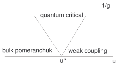
Figure 8: The phase diagram in the $u-{1\over g}$ plane. The actual phase transition takes place on the line $1/g=0$. However it can be perceived at finite $g$ if one is within the $V$-shaped quantum critical regime. In typical cases, the $1/g$ axis is replaced by the $T$ axis, where $T$ is the temperature. There a phase transition of quantum mechanical origin at $T=0$ influences the quantum critical regime at finite $T$.

Figure 8 shows what happens in a generic situation. On the $x$-axis a variable ($u_{m}$ in our case ) along which the quantum phase transition occurs. Along $y$ is measured a new variable, usually temperature $T$. Let us consider that case first. If we move from right to left at some value of $T$, we will first encounter physics of the weak-coupling phase determined by the weak-coupling fixed point at the origin. Then we cross into the critical fan (delineated by the $V$-shaped dotted lines), where the physics is controlled by the quantum critical point. In other words we can tell there is a critical point on the $x$ -axis without actually traversing it. As we move further to the left, we reach the strongly-coupled symmetry-broken phase, with a non-zero order parameter.

In our problem, $1/g^{2}$ plays the role of $T$ since $g^{2}$ stands in front of the effective action for $\sigma$. (Here $g$ also enters at a subdominant level inside the action, which makes it hard to predict the exact shape of the critical fan.) The bottom line is that we can see the critical point at finite $1/g$. In addition one can also raise the actual temperature $T$ or bias voltage to see the critical fan.

Subsequent work has shown, in more familiar examples than Landau interactions, that the general picture depicted here is true in the large $g$ limit: upon adding sufficiently strong interactions the Universal Hamiltonian gives way to other descriptions with broken symmetryMurthy (2004).

It was mentioned earlier that the critical coupling $u^{*}$ (a nonuniversal quantity) cannot be reliably predicted in the large $g$ limit. It has become clear from numerical work Adam, Brouwer and Sharma (2003) that it coincides with the bulk coupling for the Pomeranchuk transition. In other words, when we cross over to the left $u^{*}$, the size of the order parameter very rapidly grows from the mesoscopic scale of order $E_{T}$ to something of order the Fermi energy $E_{F}$. However the physics in the critical fan as well as the weak coupling side is as described by the RMT+RG analysis. The strong coupling side has to be reworked from scratch since the Fermi surface assumed in the RG that came down to $E_{T}$ is has suffered huge deformations (in the scale of $E_{F}$).

VI Summary and conclusions

Our goal was to understand the transport properties of a quantum dot- an island that electrons could tunnel on to and tunnel out of. As one varies the gate voltage $V_{g}$ between the leads and the dot, the conductance $G$ exhibits isolated peaks of varying location and height. What we wanted was a statistical description of these features as exhibited by an ensemble of similar dots. The dot was assumed to be so irregular and the classical motion so chaotic, that the only conserved quantity was energy.

To get warmed up, we asked how we would go about addressing the problem if electron-electron interactions could be neglected. It was seen that peak heights and positions could be determined from the wavefunctions and energy levels. These in turn could be determined by RMT given just the mean level spacing. In the non-interacting theory, $P(\Delta)$, the distribution of differences in $V_{g}$ between successive peaks, was the same as $P({\delta})$, the distribution of spacings between successive levels in the dot.

Actual comparison of these two distributions showed a clear disagreement, which represented a failure, not of RMT, but of the assumption of non-interacting electrons. So interactions had to be included.

The coulomb interaction implied that adding an electron to the dot would cost not just the gap to the next empty level, but an additional energy due to repulsion by the $N$ electrons already in the dot. This charging energy could be accounted for by adding a term $u_{0}N^{2}$ to the second quantized Hamiltonian. In the presence of spin, we also needed to add a term $-J_{0}S^{2}$ to represent the exchange interaction. The final result was $H_{U}$, the universal Hamiltonian. While the success of this model is unquestioned at moderate values of interaction strength, some arguments for why this had to be the right answer, and why other interactions could be neglected because their ensemble averages vanished were not persuasive. We asked if there was there a better way to understand the success of $H_{U}$.

It was pointed out that the RG was such a way since it offered an unbiased procedure for determining which interactions were really important in deciding low energy properties like the ground state and its low energy excitations. In the RG approach one divided the variables into two sets: $x$, which we cared about, and $y$, which we we did not care about. In our example $x$ was the low energy region (near the Fermi energy) and $y$ everything else. One then eliminated or integrated out the $y$’s to obtain an effective theory of just $x$, which gave the same answers in the $x$-domain as the original one. In this process some initially very impressive couplings could fade into oblivion (irrelevant) while tiny ones could grow in size (relevant) and some could remain fixed (marginal). In any event we could see which couplings really mattered. We saw that while the RG concept itself was non-perturbative, mode elimination was typically done perturbatively in the interaction.

The application of RG to our problem required a two-stage process as developed by Murthy and Mathur. First one ignores disorder and finite size and eliminates high energy modes outside the Landau band, a region of width $E_{L}$ measured from the Fermi surface. Here we know from past RG work on clean bulk systems that we must invariably end up with the Landau interaction $u({\theta})$. But we are not done yet. Although the Landau scale $E_{L}$ is much smaller than $E_{F}$, the Fermi energy, it does not vanish for infinite system size. So $E_{T}$, which vanishes as $1/L$, lies even closer to $E_{F}$. So we need to renormalize down from $E_{L}$ to $E_{T}$. During this process the Landau parameters could renormalize in a way we cannot determine. (Though in a clean system $u_{m}$ are strictly marginal, once we approach $E_{T}$ and take disorder seriously, a nonzero flow is guaranteed. ) So one begins at $E_{T}$ by writing the (renormalized) Landau interaction in the disordered single-particle basis ${\alpha}$ and eliminating the ${\alpha}$ states to determine the fate of the Landau interactions. It was found that only $u_{0}$ and $J_{0}$, the zeroth harmonics on the Fermi circle of the Landau interactions (for charge and spin densities), survived at the lowest energies if the starting value of $u_{m}$ was either positive or not below a negative coupling $u_{m}^{*}$, of order unity. Thus the low energy fixed point for this range of initial coupling was just $H_{U}$, the universal Hamiltonian. In addition to providing this justification of the emergence of $H_{U}$, the calculation also suggested that for $u_{m}<u_{m}^{*}$ the system underwent a phase transition in the $g\to\infty$ limit. Before discussing the phase transition, let us recall how the calculation of the ${\beta}$-function was done.

In any interacting field theory with some coupling $u$, one computes a physical quantity like a scattering amplitude in a power series in $u$, starting with $u$ itself, followed by loop diagrams of increasing complexity. These loops involve momentum or energy sums (or integrals) up to some cut-off ${\Lambda}$. Clearly if the sum of all these terms has to be independent of ${\Lambda}$ (as is the physical scattering amplitude) then $u$ itself must become $u({\Lambda})$ and vary with ${\Lambda}$ in such a way as to keep the series as a whole ${\Lambda}$-independent. Conversely it is possible to determine $u({\Lambda})$ by drawing diagrams to some order in $u$ making this demand. In our problem, the computation of ${\beta}(u)=-{\Lambda}du/d{\Lambda}$ for any one specific dot required knowledge of the wave-functions and energy levels lying within $E_{T}$. But thanks to self-averaging, one could replace the ${\beta}$- function for the given dot by its ensemble average. The zeroes of this ${\beta}$-function are what showed $H_{U}$ to be a fixed point (at the origin) and $u_{m}^{*}$ to be the the critical point for the phase transition.

This clever calculation was nonetheless a weak-coupling analysis predicting a phase transition at strong coupling. Was the transition real and if so, what was on the strong coupling side? It was here that the $1/N$ technique came in. In the large $g$ limit one could show that all physics could be extracted in a saddle point calculation of the $1/N$ type for any coupling $u_{m}$. In contrast to theories where there were $N$ equivalent species, here we had $g$ fermions with different energies and matrix elements. However, thanks to disorder self-averaging, one could pull out a $g^{2}$ in front of the action for the Hubbard-Stratonovic field $\sigma$. The saddle point theory confirmed the fixed point nature of $H_{U}$ for $u_{m}^{*}<u_{m}<\infty$ and the transition at $u_{m}^{*}$. Furthermore we could see beyond the transition to the other side: here $\sigma$ acquired an average (a disordered version of the Pomeranchuk transition in clean systems) and produced many attendant consequences like time-reversal breaking. However the ”exact” critical point $u_{m}=u_{m}^{*}$ of this calculation was not a directly measurable quantity since the saddle point theory had as its input, not the Landau interaction defined at $E_{L}$, but what it had evolved into, between $E_{L}$ and $E_{T}$. This was a no man’s land where disorder was too strong to be ignored, but not strong enough to use RMT since we were not within $E_{T}$ making the flow intractable. However clever arguments of Adam et a show that the transition occurs at the bulk critical value of $u_{m}=1$.

Since the phase transition occurs only at infinite $g$ (a finite system always has finite $g$ and cannot have a transition), it might seem that our study of it was academic. This is not so, and the reason is the same as in quantum critical phenomena. Recall that there, a quantum phase transition at $T=0$ as a function of some coupling $u=u^{*}$ can be felt even at $T>0$ inside a $V$-shaped region called the quantum critical region. Here $g^{2}$ plays the role of $1/T$ as a prefactor in the action. Thus we can see the effects of the critical point even at finite $g$ and over a wide range of coupling.

I began with the ominous remark that three obstacles are ganged up here: randomness, strong interactions and finite size. Yet they ended up being benign: randomness and finite size led to a finite Thouless band within which we could use RMT and ply our trade, while strong interactions led to an interesting phase transition. As for the RG, it had to be invoked in the first stage as we came down to $E_{L}$ using the clean system RG to end up with the Landau interactions. At this point we could either use perturbative self-averaged RG inside $E_{T}$ or better still, use the self-averaged $1/N$ method to solve the model by saddle point.

This colloquium has emphasized what I find most beautiful about this problem: the confluence of physical complications and the interplay of diverse techniques that lead to a solution. Of necessity it has been sparse on phenomenology. However, armed with the ideas explained here you are ready to remedy this, following any number of the excellent references mentioned in the text.

It will be very interesting if experimentalists unearthed the phenomena chronicled here by studying dots with strongly interacting electrons, a possibility more readily realized than in the bulk since electron density in dots can be controlled by gates. Stay tuned for these results.

References

- Adam, Brouwer and Sharma (2003) Adam, S., P.W. Brouwer, and P. Sharma, 2003, Phys. Rev. B 68, 241311.
- Aleiner et al. (2002) Aleiner I.L., P.W. Brouwer, and L.I. Glazman , 2002, Phys. Rep. 358, 309, (a review of ).
- Alhassid (2000) Alhassid, Y. , 2000, Rev. Mod. Phys. 72, 2000 (a review of dots in general).
- Andreev and Kamenev (1998) Andreev, A.V. and A. Kamenev, 1998, Phys. Rev. Lett. 81, 3199.
- Baranger, Ullmo and Glazman (2000) Baranger, H.U., D. Ullmo, and L.I. Glazman, 2000, Phys. Rev. B 61, 2425.
- Browuer, Oreg and Halperin (1999) Brouwer, P.W., Y. Oreg, and B.I. Halperin 1999, Phys. Rev. B 60, 13977.
- Chakravarty et al. (1988) Chakravarty, S., B.I. Halperin, and D.R. Nelson, 1988, Phys. Rev. B 39, 2344.
- Chang et al. (1996) Chang A.M., P.W. Brouwer, H.U. Baranger , L.N. Pfeiffer ,K.W. West , and T.Y. Chang ,1996, Phys. Rev. Lett.. 76, 1695.
- Folk et al. (1996) Folk J.A., S.R. Patel, S.F. Godjin , A.G. PHuibers ,S.M. Cronenwert , and C.M. Marcus ,1996, Phys. Rev. Lett.. 76, 1699.
- Gross and Neveu (1974) Gross, D.J. , A., Neveu , 1974, Phys. Rev. D 10, 3235.
- Guhr, Muller-Groeling and Weidenmuller (1998) Guhr, T. , A., Muller-Groeling and H., Weidenmuller 1998, Phys. Rep. 299, 189 (a review of RMT).
- Jalabert, Stone and Alhassid (1992) Jalabert, R.A. , A.D., Stone , andY., Alhassid , 1992, Phys. Rev. Lett. 68, 3468.
- Kurland,Aleiner and Altshuler (2000) Kurland, I.L., I.L. Aleiner, and B.L. Altshuler, 2000, Phys. Rev. B 62, 14886.
- Landau (1956) Landau, L.D. , 1956, Sov. Phys. JETP 3, 920.
- Mehta (1991) Mehta, M.L. , 1991, Random matrices (Academic Press, San Diego.
- Merlin (2000) Merlin, A. D. , 2000, Phys. Rep. 326, 259, (a review of RMT and dots).
- Murthy and Mathur (2002) Murthy, G. , H., Mathur , 2002, Phys. Rev. Lett. 89, 126804.
- Murthy and Shankar (2003) Murthy, G. and R. Shankar, 2003, Phys. Rev. Lett. 90, 066801.
- Murthy et al. (2004) Murthy, G., R. Shankar, D. Herman, and H. Mathur, 2004, Phys. Rev. B 69, 075321.
- Murthy (2004) Murthy, G., 2004, Phys. Rev. B 70, 153304.
- Murthy, Shankar and Mathur (2005) Murthy, G. R. Shankar and H. Mathur, 2005, Phys. Rev. 72, 075364.
- Oganesyan, Kivelson and Fradkin (2001) Oganesyan, V., S.A. Kivelson, and E. Fradkin, 2001, Phys. Rev. B 64, 195109.
- Oreget al. (2001) Oreg, Y.,P.W., Brouwer,X., Waintal and B.I. Halperin, 2001, eprint cond-mat/0109541, (a review of ).
- Pomeranchuk (1958) Pomeranchuk, I.I. , 1958, Sov. Phys. JETP 8, 361.
- Sachdev (1994) Sachdev, S., 1999, Quantum phase transtions (Cambridge University Press, UK).
- Shankar (1994) Shankar, R., 1994, Rev. Mod. Phys. 66, 129, (a review of RG, fermionic path inegrals, Luttinger liquid).
- Varma (1999) Varma, C.M. , 1999, Phys. Rev. Lett. 83, 3538.