Modeling Wildland Fire Propagation
with Level Set Methods

Level set methods are versatile and extensible techniques for general front tracking problems, including the practically important problem of predicting the advance of a firefront across expanses of surface vegetation. Given a rule, empirical or otherwise, to specify the rate of advance of an infinitesimal segment of firefront arc normal to itself (i.e., given the firespread rate as a function of known local parameters relating to topography, vegetation, and meteorology), level set methods harness the well developed mathematical machinery of hyperbolic conservation laws on Eulerian grids to evolve the position of the front in time. Topological challenges associated with the swallowing of islands and the merger of fronts are tractable.

The principal goals of this paper are to: collect key results from the two largely distinct scientific literatures of level sets and firespread; demonstrate the practical value of level set methods to wildland fire modeling through numerical experiments; probe and address current limitations; and propose future directions in the simulation of, and the development of decision-aiding tools to assess countermeasure options for, wildland fires. In addition, we introduce a freely available two-dimensional level set code used to produce the numerical results of this paper and designed to be extensible to more complicated configurations.

Keywords: Wildland firespread, level set methods, Multivac software

1 Introduction

Wildland fire modeling has received attention for decades, due to the sometimes disastrous consequences of large fires, and the tremendous costs of often ineffectual, possibly even counterproductive firefighting [Pyne,, 2004]. For the practically important scenario of wind-aided firespread, one seeks a computationally efficient model, useful not only offline (for pre-crisis planning, e.g., placement of access roads, firebreaks, and reservoirs, and scoping of fuel-reduction burning, and post-crisis review, e.g., personnel training, litigation), but also during a crisis (i.e., real-time guidance for evacuation and firefighting). For computational efficiency, such that the benefits of ensemble forecasting [Palmer et al.,, 2005] are readily accessible from a model, advantage should be taken of the inherent scale separation of: (1) the kilometer-and-larger, landscape-dominated scales of the local atmospheric dynamics; and (2) the one-meter-and-smaller scales of the local combustion dynamics. Even with advanced techniques and access to exceptional contemporary computing facilities, numerical simulations (of turbulent flows) that proceed from fundamental principles are challenged to resolve accurately in real time phenomena with spatial scales spanning much more than two orders of magnitude [H.R. Baum, private communication]. Thus, the feasibility of a direct numerical simulation encompassing the multivaried processes of wildland fire propagation [Coen,, 2003] may be decades off [Jenkins et al.,, 2001]. Moreover, at least many attempts (albeit usually problematic) at parameterization of subgridscale phenomena in terms of gridscale variables have been undertaken by meteorologists for cumulus convection, turbulent transport, and radiative transfer. However, meteorologists have extremely limited experience with the parameterization of combustion dynamics for weather-dependent wildland firespread; even if such parameterization be possible, it remains unknown. Furthermore, data collection in wildland fires is so piecemeal, irregular, and of uncertain accuracy that, for many years to come, the data better suit reinitialization of a simplistic model than assimilation into an ongoing calculation with a highly detailed model.

Accordingly, in this study, attention is focused on a minimalist treatment of the firefront, idealized as an interface between expanses of burned and unburned vegetation. This treatment is consistent with the typically limited, only gross characterization available for the vegetation at issue, since the vagaries of ignition events are difficult to anticipate, and maintaining an updated inventory for the huge area of wildlands in (say) the USA is daunting. This simplistic interfacial approach to the fire dynamics, easily executed in minutes on a laptop given the requisite meteorological and other input fields, reserves computational resources for the difficult, more critical, and mostly yet-to-be-undertaken landscape-scale weather forecasting targeted for real-time wildfire applications.

The upshot is that simple persistence models are adopted for the wind field (and thermodynamic variables) in the study undertaken here. Also, attention is limited to a one-way interaction between the meteorology and the firespread, though future extension to two-way interaction by use of an iterative procedure may be envisioned. Simplistic modeling still may provide the key macroscopic fire behavior sufficiently accurately for practical purposes (including estimates of smoke and pollutant generation), even for circumstances for which the simplification is not formally justifiable. In fact, observational data of wind-aided firefront progression in wildland are today typically sparse, so that not much more than the output of a simplistic model can be meaningfully validated and tuned. Moreover, the use of relevant mathematical methods to perform model selection, to carry out efficient parameter estimation, and to account for the uncertainty in predictions is facilitated by focusing on less detailed models with fewer parameters. In this paper, we mainly address the first step, which is to achieve proper forward simulations.

One of the most widely used models was devised by Rothermel [Rothermel,, 1972] to predict the rate of firespread, with focus on the head of a wind-aided fire. Because predictions of the Rothermel treatment have been found to be at odds with some observations, efforts to improve this spatially one-dimensional semi-empirical treatment, and to supplement the data upon which it is based, have been undertaken, especially in recent years [Carlton,, 2003]. Extension from a focus exclusively on the head of the fire seeks to evolve the configuration of the entire fire perimeter, possibly of multiple fire perimeters. In this study, and typically, the firefront, even a moderate fraction of an hour after a localized ignition in fire-prone vegetation, is taken to be a closed curve projected on a plane (the ground may not be flat). Such simulations of firespread have been performed [Finney,, 1998] with the so-called marker technique, which discretizes a front into a set of marker particles, and advances the front through updates of the particle positions. Parenthetically, as a problematic step, the updating by Finney takes each marker on the front to evolve identically to an idealization of how a front evolves from a single isolated ignition site in an unbounded expanse of vegetation, in the presence of a wind. In any case, even though applied projects have supported software development [Finney,, 1998], still from a computational point of view, only a few, largely equivalent methodological developments have been undertaken [e.g. André et al.,, 2006]. In this paper, we apply level set methods [Osher and Sethian,, 1988; Sethian,, 1999] to calculate firefront evolution.

In Section 2, we introduce wildland firespread models, especially a semi-empirical, equilibrium-type model proposed in Fendell and Wolff, [2001] for wind-aided firespread across surface-layer, chaparral-type, burning-prone vegetation. (In commonly adopted equilibrium-type models, the firespread rate depends on only the parametric values holding locally and instantaneously, so the firespread rate is taken to adjust indefinitely rapidly to any temporal and spatial change.) Section 3 provides a brief introduction to level set methods. Section 4 describes the Multivac level set package that has been applied in this paper to the firespread problem. A quick description of its performance is presented in Section 5. Finally, results of firespread simulations with different idealized environmental conditions are reported in Section 6.

2 Front Propagation Functions for Wildland Fires

Even if theory and/or measurement furnished complete, perfect knowledge of the topography, vegetation, and meteorology at a site at a given time (e.g., furnished the locally pertinent values of all parameters in functional forms capable of representing these three types of input), still one currently possesses very incomplete, imperfect knowledge of the “rules” that would yield the physically observed rate of firespread from the input. Achieving knowledge of firespread “rules” sufficiently accurate for practical purposes may well lag emplacing means for observing and collecting exhaustive input data.

As already noted, a fire-growth simulation such as FARSITE [Finney,, 1998] seems unlikely to reach its potential as long as it seeks to describe the rate of firespread at all orientations to the direction of the sustained low-level ambient wind from spread-rate modeling focused on the direction of the wind [e.g. Rothermel,, 1972]. On the other hand, posing a different rule for the spread rate at every possible orientation to the wind defeats the goal of simplicity.

2.1 Wind-aided wildland fire spread

Fendell and Wolff [Fendell and Wolff,, 2001] addressed this dilemma in developing a model dedicated to wind-aided wildland fires that spread rapidly over level terrain with dry, moderately sparse fuel, taken here to be uniformly distributed to permit concentration on wind effects. Parenthetically, for consistency with modeling in which the firefront is idealized as an interface moving according to a semi-empirical rule, only a minimal amount of information about the surface-layer fuel is required, mainly the mass loading consumed with firefront passage (“available”-fuel loading).

The Fendell and Wolff model focuses on front velocities at the rear of the front (where propagation is against the wind), at the head of the front (where propagation is with the wind), and on the flanks (where propagation is across the wind direction) – see Figure 1. The firespread velocities primarily depend on the wind velocity $U$. At the rear, the front advances relatively slowly against the oncoming wind, since hot combustion products tend to be blown over an already burned area. The velocity at the rear is denoted $\varepsilon(U)$. At the head, the velocity $h(U)$ is relatively large, since hot combustion products tend to be blown over a yet-to-burn area, in which discrete fuel elements are heated toward ignition by convective-conductive transfer. Both analytic modeling and laboratory experiments have shown that $h(U)$ is roughly proportional to $\sqrt{U}$ [Wolff et al.,, 1991]. At the flanks, the (spread-aiding) wind component along the normal to the front is zero, but observationally the front advances faster than in the absence of wind. As a speculation, a more meticulous treatment would find that, at the nominal flank, the configuration is convoluted, and firespread is alternately with and against the wind. Of course, were the wind direction constant, limiting attention to the head would seem adequate, but, in fact, change in wind direction may (rapidly) result in an interchange of the locations of the flank and head – an interchange sometimes associated with tragic consequence for firefighters.

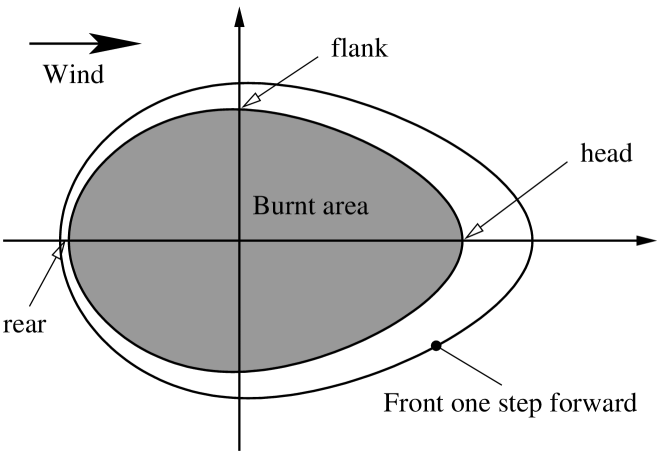
Figure 1: Fendell and Wolff model introduces velocities at the rear (against the wind), at the head (in the wind direction) and at the flanks. [Fendell and Wolff,, 2001]

The velocities (the terminology henceforth adopted, for brevity, in place of firespread rates) proposed in Fendell and Wolff, [2001] are

$$\varepsilon(U)=\varepsilon_{0}\exp(-\varepsilon_{1}U),\quad f(U)=\varepsilon_{0}+c_{1}U\exp(-c_{2}U),\quad h(U)=\varepsilon_{0}+a\sqrt{U},$$ (1)

where $\varepsilon_{0}$, $\varepsilon_{1}$, $c_{1}$, $c_{2}$ and $a$ are parameters (with readily inferred dimensionality) depending on the mass loading of fuel and other parameters characterizing the fuel bed, but independent of $U$.

The velocity is then provided at any point on the front through a “trigonometric interpolation”:

$$\begin{array}[]{l}F(U,\theta)=f(U\sin^{m}\theta)+h(U\cos^{n}\theta)\quad\textrm{if $|\theta|\leq\frac{\pi}{2}$},\\ F(U,\theta)=f(U\sin^{m}\theta)+\varepsilon(U\cos^{2}\theta)\quad\textrm{if $|\theta|>\frac{\pi}{2}$},\end{array}$$ (2)

where $\theta$ is the angle between the wind direction and the normal to the front. We set $m=2$. In this paper, parameter $n$ is set to $\frac{3}{2}$ and is significant since it determines the overall shape of the front from the flanks to the head.

To summarize, the velocity is, for all $U\in\mathbb{R}_{+}$ and $\theta\in]-\pi,\pi[$,

$$\begin{array}[]{rl}F(U,\theta)=&\varepsilon_{0}\sin^{2}\theta+c_{0}U\sin^{2}\theta\hskip 1.42262pt\exp\left(-c_{1}U\sin^{2}\theta\right)\\ &+\left\{\begin{array}[]{llll}\displaystyle\varepsilon_{0}\cos^{2}\theta+a\sqrt{U}\cos^{n}\theta&\textrm{if $|\theta|\leq\frac{\pi}{2}$}\\ \displaystyle\varepsilon_{0}\cos^{2}\theta\hskip 1.42262pt\exp\left(-\varepsilon_{1}U\cos^{2}\theta\right)&\textrm{if $|\theta|>\frac{\pi}{2}$}\end{array}\right..\end{array}$$ (3)

2.2 Simplified model

Based on the numerical experiments carried out with the level set code Multivac (Section 4), the model (3) proposed in Fendell and Wolff, [2001] has been modified. First, the parameter $n$ has been set to $\frac{3}{2}$ instead of $1$. Second, the model has been simplified without losing its main features, primarily the overall shape of the firefront. The new model reads

$$\begin{array}[]{ll}F(U,\theta)=\varepsilon_{0}+c_{1}\sqrt{U}\cos^{n}\theta&\quad\textrm{if $|\theta|\leq\frac{\pi}{2}$},\\ F(U,\theta)=\varepsilon_{0}(\alpha+(1-\alpha)|\sin\theta|)&\quad\textrm{if $|\theta|>\frac{\pi}{2}$},\end{array}$$ (4)

where $\alpha\in[0,1]$ is the ratio between the velocity at the rear ($\alpha\varepsilon_{0}$) and the velocity at the flanks ($\varepsilon_{0}$). Velocities at the rear and at the flanks no longer depend on the wind, since their dependence on the wind speed is hard to model accurately and has little impact on the overall front location. The velocity at the head is the same as in the “full” model (3).

The simplified model is easier to tune, either via direct trials or with systematic methods for parameter estimation (which may require derivatives of the model with respect to its parameters). All results in this paper are for the simplified model. However, results for the “full” model would appear roughly the same.

3 Level Set and Fast Marching Methods

First introduced in Osher and Sethian, [1988], level set methods are Eulerian schemes for tracking fronts propagating according to a given speed function. In this section, we explain basic features of the level set methods used for firespread modeling.

3.1 Mathematical basis and technique

3.1.1 Definitions

Assume the front evolves from the initial time $t=0$ to the final time $t=T_{f}$. For all $t\in\left[0,T_{f}\right]$, the front at time $t$ is the set of points (in $\mathbb{R}^{N}$) $\Gamma(t)$. We define $\Gamma_{0}=\Gamma(0)$ as the initial front.

For all $t\in\left[0,T_{f}\right]$, each point $X\in\Gamma(t)$ with a well-defined normal moves in the direction normal to the front with a given speed $F(X,\Gamma,t)$. Notice that $F$ may depend on the position, on the time and on local properties of the front itself (certainly the normal direction, not always defined, and possibly the local curvature or other properties).

The problem is to approximate $\Gamma:\left[0,T_{f}\right]\rightarrow\mathbb{R}^{N}$, given $\Gamma_{0}$ and $F$.

3.1.2 Strategy

The main idea is to evolve a function $\varphi:\mathbb{R}^{N}\times\left[0,T_{f}\right]\rightarrow\mathbb{R}$ such that

$$\forall\hskip 1.99168ptt\in\left[0,T_{f}\right]\qquad\Gamma(t)=\left\{x\in\mathbb{R}^{N}\Big{/}\varphi(x,t)=0\right\}.$$ (5)

$\varphi$ is called the level set function. At any time, the zero level set of $\varphi$ is the front itself. A priori, $\varphi$ could be any function satisfying equation (5). However, some assumptions (e.g., smoothness) and practical issues (e.g., initialization of $\varphi$) make it convenient to define $\varphi$ as the signed distance to the front.

Then, if $d$ is the Euclidean distance on $\mathbb{R}^{N}$, we define, for any given curve $\Upsilon$, the distance $d_{\Upsilon}$ to $\Upsilon$:

$$\forall\hskip 1.99168ptx\in\mathbb{R}^{N}\qquad d_{\Upsilon}(x)=\min\left\{d(x,P)\Big{/}P\in\Upsilon\right\}.$$ (6)

Hence the signed distance $\varphi$ for all $x\in\mathbb{R}^{N}$ and $t\in\left[0,T_{f}\right]$:

$$\varphi(x,t)=\left\{\begin{array}[]{ll}d_{\Gamma(t)}(x)&\textrm{if $x$ lies outside the front $\Gamma(t)$}\\ -d_{\Gamma(t)}(x)&\textrm{if $x$ lies inside the front $\Gamma(t)$}\\ \end{array}\right..$$ (7)

It can be shown that $\varphi$ obeys the equation

$$\forall\hskip 1.99168ptx\in\mathbb{R}^{N}\quad\forall\hskip 1.99168ptt\in[0,T_{f}]\qquad\varphi_{t}(x,t)+F(x,\varphi(\cdot,t),t){\|\nabla_{x}\varphi(x,t)\|}_{2}=0,$$ (8)

where the velocity $F$ is now defined everywhere in $\mathbb{R}^{N}$ and depends on the front through its dependence upon $\varphi$. Details may be found in Sethian, [1999].

Recall that $\varphi(\cdot,0)$ is known as well as $\Gamma_{0}$; $\varphi(0)$ is the signed distance to $\Gamma_{0}$:

$$\forall\hskip 1.99168ptx\in\mathbb{R}^{N}\quad\varphi(x,0)=\left\{\begin{array}[]{ll}d_{\Gamma_{0}}(x)&\textrm{if $x$ lies outside the front $\Gamma_{0}$}\\ -d_{\Gamma_{0}}(x)&\textrm{if $x$ lies inside the front $\Gamma_{0}$}\\ \end{array}\right..$$ (9)

Equations (8) and (9) define the initial-value problem that is to be solved. Zero level sets of $\varphi$ yield the front points.

This nonstationary problem involves the Hamilton-Jacobi equation (8). There may be multiple solutions to this equation. P.-L. Lions and M. G. Crandall defined the so-called “viscosity solution” of Hamilton-Jacobi equations [Lions,, 1982; Crandall and Lions,, 1983], which turns out to be the unique physical solution for which we search. Under given assumptions (mainly on the speed function $F$), existence and uniqueness of the viscosity solution of the problem (8)–(9) can be proved.

3.2 Advantages and disadvantages of level set methods

Several methods may be relevant to simulate the propagation of firefronts. One may want to use marker techniques, in which the front is discretized by a set of points. At each time step, each point is advanced according to the speed function. This Lagrangian methodology leads to low-cost computations, but requires care in the handling of topological changes.

Volume-of-fluid methods represent the front by the amount of each grid-cell that is inside the front. In each cell, the front is approximated by a straight line (horizontal or vertical, in most methods). Such methods can deal with topological changes, but the front representation can be inaccurate. In wildland firespread, the direction normal to the front is crucial because of the wind-direction-dependent speed function (see Section 2).

Level set methods automatically deal with topological changes that occur in wildland firespread, such as fronts merging and front convergence (in connection with unburnt “islands”). The level set description enables a fair estimate of the normal to the front, making it well suited to the fire propagation problem.

However, level set methods have disavantages. First, they embed the front in a higher-dimensional space. Helpfully, the narrow band level set method [Adalsteinsson and Sethian,, 1995] is an efficient algorithm which almost decreases the problem dimension by one. Moreover, when it can be used, the fast marching method [Sethian,, 1996] provides a highly efficient algorithm.

The main reservation may be the lack of proof of convergence of numerical schemes for certain problems. For a given class of speed functions, the problem (8)–(9) may routinely be solved numerically [Crandall and Lions,, 1984]. However, no proof of convergence in mesh parameter or time step is yet available for some situations.

3.3 Quick review of numerical approximations

Numerical approximation to solutions of Hamilton-Jacobi equations is closely related to numerical approximation to hyperbolic conservation laws. The point is to introduce a numerical Hamiltonian to approximate the Hamiltonian $H=F\cdot{\|\nabla_{x}\varphi\|}_{2}$.

Crandall and Lions have proven that, for given Hamiltonians and initial conditions, a consistent, monotonic and locally Lipschitzian numerical Hamiltonian yields a solution that converges to the viscosity solution. Formal results may be found in Crandall and Lions, [1984] and Souganidis, [1985].

In one dimension, $\varphi_{t}+H(\nabla_{x}\varphi)=0$ may lead to the following approximation:

$$\varphi^{n+1}_{j}=\varphi^{n}_{j}-\Delta t\hskip 2.84526ptg\left(\frac{\varphi_{j+1}-\varphi_{j}}{\Delta x},\frac{\varphi_{j}-\varphi_{j-1}}{\Delta x}\right).$$ (10)

For instance, if the Hamiltonian is not convex, the Lax-Friedrichs scheme may be used; then, the numerical Hamiltonian is

$$\forall\hskip 1.99168pta,b\in\mathbb{R}\qquad g(a,b)=H\left(\frac{a+b}{2}\right)-\vartheta\frac{b-a}{2},$$ (11)

where the monotonicity is satisfied on $[-R,R]$ if $\displaystyle\vartheta=\max_{-R\leq a\leq R}|H^{\prime}(a)|$.

Several schemes have been developed, from simple and efficient schemes as that of Engquist-Osher to high-order essentially nonoscillatory schemes [Osher and Shu,, 1991].

3.4 Overview of complexity issues

Let the mesh (in $\mathbb{R}^{N}$) be orthogonal with $M$ points along each direction. Assume that the front is described by $\mathcal{O}(M^{N-1})$ points. The narrow band level set method makes it sufficient to update the level set function only in a narrow band (of width $k$) around the front. For each time step, the complexity of the algorithm is therefore $\mathcal{O}(kM^{N-1})$.

For an explicit temporal discretization the number of iterations is related to the Courant-Friedrichs-Lewy condition. Along $x$, the Courant number must be less than $1$:

$$\frac{\max\left|H^{\prime}\right|\Delta t}{\Delta x}\leq 1.$$ (12)

Usually, controlling the accuracy of approximation is subordinate to space discretization, which means that the time step is adjusted so that the Courant number is taken close to $1$.

Calculations may sometimes be sped up by reformulating the level set problem as a stationary problem. This leads to the so-called fast marching method [Sethian,, 1996]. Nevertheless, restrictions on the Hamiltonian prevent the use of this technique for some applications. The work of Sethian and Vladimirsky has overcome some limitations [Sethian and Vladimirsky,, 2001], but restrictive conditions still remain (e.g., convexity of the Hamiltonian).

4 Code

4.1 Introduction to the Multivac level set package

Multivac is a level set package freely available (under the GNU GPL license) at http://vivienmallet.net/fronts/. It is designed to be both efficient and extensible, so that it may be used for a large range of applications. To achieve these goals, Multivac is built as a fully object-oriented library in C++.

Multivac was designed independently of the firespread application described herein, but easily enabled firespread simulations, and is presently distributed with firespread-motivated functions. It has also been used in modeling the growth of Si-based nanofilms [Phan and Mallet,, 2003] and image segmentation.

The latest stable version available at the time of submission is Multivac 1.10.

4.2 Structure

The modularity of Multivac comes from its object-oriented framework, in which the main components of a simulation have been split into an equal number of objects. A simulation is defined by the following objects:

• the mesh;

• the level set function;

• the velocity, which provides the propagation rate of the front according to its position, its normal, its curvature, and the time;

• the initial front;

• the initializer, which manages first initializations and initializations required by level set methods (e.g., the narrow band reconstruction);

• the numerical scheme, which advances the front in time;

• the output management.

For each item, a set of classes with a common interface is available. For instance, several speed (i.e., propagation rate) functions are available through several classes, e.g. CConstantSpeed or CFireModel. All speed functions have the same interface, which allows users to define their own speed function on the same basis. The user principally provides speed rates as a function of the position, the time, the normal to the front and the curvature (these values are computed by Multivac itself).

4.3 Calling sequence

The whole is managed by an object of the class CSimulator. This object simply calls the initializer to perform the first initializations. Then it manages the loop in time (or iterations, in the case of the fast marching method) into which the numerical scheme is called to advance the front. The initializer is called again to reinitialize the signed distance function for the new step, and the object dedicated to post-processing requirements is called to save any needed data.

In each step, objects communicate with one another through methods (i.e., functions) of their interface. For example, the velocity object provides speed rates to the numerical scheme.

4.4 Overview of available classes

Multivac package (version 1.10) includes several classes which are listed in Table 1.

Category	Available classes
Mesh	Orthogonal mesh
Level set function	Defined on an orthogonal mesh
Velocity	Constant speed
	Piecewise constant speed
	Fire model
	Simplified fire model
	Image intensity
	Image gradient
Initial front	Circle
	Two or three circles
	One or two circles with an island inside
	Front defined by any set of points
Initializer	Basic initialization (no velocity extension)
	Extends the velocity with the closest
	neighbor on the front
Numerical scheme	Engquist-Osher, first order
(narrow band)	Lax-Friedrichs, first order
	Engquist-Osher, ENO, second order
	Chan-Vese algorithm [Chan and Vese,, 2001]
Numerical scheme	Engquist-Osher, first order
(fast marching)

Table 1: Basic classes available in Multivac 1.10.

4.5 Other strengths, limitations and future work

Multivac takes advantage of C++ exceptions to track errors, and several debugging levels are defined, from a safe mode, in which all is checked, to a fast mode, in which performance is the primary concern.

There are currently two main limitations. First, Multivac deals only with uniform orthogonal meshes. However, extensions of level set methods to unstructured meshes exist (e.g., Barth and Sethian, [1998]) and they could be implemented within the Multivac framework. Adaptively refined meshes are also accommodated with additional mathematical complexity, though the implementation effort would be substantial. Second, Multivac deals only with two-dimensional problems.

Work is planned to allow inverse modeling (parameter estimation based on data assimilation) within the framework of Multivac. The main idea is to replace the class CSimulator with a class dedicated to inverse modeling. Preliminary results show the framework extendibility, but this capability is not yet available in distributed versions. Future versions should include this feature, based on an innovative method for integrating sensitivities along with the front itself.

5 Complexity and Convergence Studies

5.1 Convergence studies

In this section, we report convergence studies that are necessary to validate the code. As in Adalsteinsson and Sethian, [1998], tests are carried out for a circle that expands in time with a unitary velocity. Details of the simulation are summarized in Table 2.

Data	Value	Comment
Domain	$\Omega=[0,3]\times[0,3]$
Initial front	Circle
Circle center	$\left(x_{c},y_{c}\right)=\left(1.5,1.5\right)$	Domain center
Initial circle radius	$r_{initial}=0.5$
Final circle radius	$r_{final}=0.9$
Velocity	$F=1.0$	Constant
Duration	$T_{f}=0.4$
Time step	$\Delta t=10^{-4}$

Table 2: Simulation test-case.

We introduce three norms. The first is

$$e_{spatial}^{1}=|r_{simulated}-r_{final}|,$$ (13)

where $r_{simulated}$ is the simulated radius, estimated as follows:

$$r_{simulated}=\frac{1}{\mathrm{card}(\Gamma_{d})}\sum_{(x,y)\in\Gamma_{d}}\textrm{d}\left((x,y),\left(x_{c},y_{c}\right)\right),$$ (14)

where $\Gamma_{d}$ is the discretized front as returned by the simulation (at time $T_{f}$) and d is the Euclidian distance.

Additionally, if $T_{true}(x,y)$ is the time at which the front is supposed to reach the point $(x,y)$:

$$e_{time}^{2}=\sqrt{\frac{1}{\mathrm{card}(\Gamma_{d})}\sum_{(x,y)\in\Gamma_{d}}\left(T_{f}-T_{true}(x,y)\right)^{2}}.$$ (15)

The last norm is an infinity norm:

$$e_{time}^{\infty}=\max_{(x,y)\in\Gamma_{d}}\left|T_{f}-T_{true}(x,y)\right|.$$ (16)

Table 3 shows results for the first-order Engquist-Osher scheme with the narrow band method. The width of the band is 12 cells and the front lies within a band whose width is 6 cells.

$\Delta x=\Delta y$	$N_{x}=N_{y}$	$e_{spatial}^{1}$ $\left(\times 10^{3}\right)$	$e_{time}^{2}$ $\left(\times 10^{3}\right)$	$e_{time}^{\infty}$ $\left(\times 10^{3}\right)$
0.01	301	1.634	1.753	2.377
0.005	601	0.855	0.901	1.191
0.0025	1,201	0.460	0.474	0.600
0.00125	2,401	0.244	0.247	0.299

Table 3: Errors versus spatial discretization.

The first-order Lax-Friedrichs scheme and the second ENO Engquist-Osher scheme were also checked successfully. As for the second-order scheme, the full-matrix method, that is, without the narrow-band restriction, was used because the front reconstruction destroys the second-order accuracy.

5.2 Complexity issues

Multivac was compiled under Linux with GNU/g++ 3.3, and the reference simulation (see Table 2) was launched on a Pentium 4 running at 2.6 Ghz. The width of the narrow band was 12 cells and the width of the inner band, in which the front lies, was 6 cells. If $N_{x}=N_{y}=1001$ (one million cells), the $4,000$ iterations were achieved in 14 s.

The complexity of the narrow band level set method is close to $\mathcal{O}(N)$, where $N=N_{x}=N_{y}$. Table 4 shows that linear complexity of the method is not observed. Instead, the complexity seems to be $\mathcal{O}(N^{2})$. This is the complexity of the suboptimal algorithm currently used to rebuild the front. Moreover, the number of front reconstructions increases with the mesh refinement since the width of the narrow band does not change.

$\Delta x=\Delta y$	$N_{x}=N_{y}$	Timings (s)
0.03	101	0.4
0.015	201	0.9
0.01	301	1.6
0.0075	401	2.6
0.006	501	4.0
0.005	601	5.6
0.004285714	701	7.4
0.00375	801	9.5
0.003333333	901	11.9
0.003	1001	14.1

Table 4: Timings versus spatial discretization.

6 Applying Level Set Methods to Firespread Applications

6.1 Method and numerical scheme

The speed function (3) introduced in the level set equation (8) provides an Hamiltonian with nontrivial dependencies. Because of these dependencies (particularly the non-convexity of the Hamiltonian), neither the fast marching method nor its extension to anisotropic problems can be applied. The narrow-band level set method is more relevant.

A highly accurate numerical scheme is not required for the investigations reported here. The discrepancies between the numerical simulation and the exact solution should be considered in the context of other approximations: the model itself is simplistic; input parameters such as wind speed or fuel density are typically not accurately estimated; the location of the initial front introduces further uncertainties. A first-order scheme suffices for our purposes.

Since the Hamiltonian involved is not convex with respect to spatial derivatives of the level set function, the first-order Lax-Friedrichs scheme (refer to equation (11)) is well suited. To minimize introduction of diffusivity, a local Lax-Friedrichs scheme may be used as well.

As previously advocated, the timestep $\Delta t$ is chosen according to the Courant-Friedrichs-Lewy condition (12):

$$\Delta t=\frac{\alpha\Delta x}{\max\left|H^{\prime}\right|},$$ (17)

where $\alpha\leq 1$; $\alpha$ is not kept constant in the tests that we undertake. Nevertheless, the Courant-Friedrichs-Lewy condition is estimated at every iteration with an (a priori) approximation to $\max\left|H^{\prime}\right|$ along $x$ and $y$, which leads to:

$$\Delta t\leq\frac{\Delta x}{a(m+1)\sqrt{U}}.$$ (18)

The main characteristics of the simulation, including model parameters (refer to equation (3)), are gathered in Table 5.

Parameter	Value
$n$	1.5
$U$	100
$a$	0.5
$\varepsilon_{0}$	0.2
$\alpha$	0.5
$\Delta x$	$3\cdot 10^{-3}$
$\Delta y$	$3\cdot 10^{-3}$
$\Delta t$	$10^{-4}$
$T_{f}$	0.1

Parameter	Value
Domain	$\Omega=[0,3]\times[0,3]$
Initial front	Circle
Circle center	$\left(1.5,1.0\right)$
Initial circle radius	$r_{initial}=0.5$
Velocity	$F=1.0$
Duration	$T_{f}=0.1$
Time step	$\Delta t=5\cdot 10^{-5}$
Spatial discretization	$N_{x}=N_{y}=1001$

Table 5: Parameters and their default values.

6.2 Results

The simulation described by Table 5 is shown in Figure 2. The figure shows snapshots of the front, initially circular, at subsequent times, under a constant-magnitude wind blowing from left to right. Since thoroughly burnt areas cannot be burnt again (on the time scale of the simulation), the area enclosed by the front increases with time. The rear, the flanks and the head of the front are clearly identifiable.

Figure 2: Basic simulation described by Table 5.

The reference simulation is slightly modified to show the ability to deal with multiple fronts – Figure 3. It demonstrates the capability to deal with the merging of fronts (two main fronts), and to deal with the so-called islands, i.e. an unburnt area surrounded by a burnt area.

Figure 3: Two main fronts merge, and an island – the unburnt area within the biggest front – is burnt.

In Figures 4 and 5, we use the same parameters as in Table 5 but $\Delta t=2.5\cdot 10^{-5}$, and $a$ depends on $x$, $a$ being equal to $0.5$ if $x<1.7$, and $a=0.25$ (Figure 4) or $a=1.0$ (Figure 5) if $x>1.8$, and $a$ being linearly interpolated for intermediate values of $x$. Since $a$ takes into account the available fuel loading, these two simulations roughly show the influence of the inhomogeneous available fuel loading, should it increase (Figure 4) or decrease (Figure 5). The inherent decrease of the radius of curvature at the head for a constant-direction wind suggests that some vacillation of wind direction contributes when the head broadens under otherwise uniform conditions.

Figure 4: The front slows down at the head for $a=0.25$ if $x>1.8$. The final time is changed to $T_{f}=1.5$.

Figure 5: The front advances faster at the head for $a=1.0$ if $x>1.8$.

Figure 6 shows the impact of a rotating wind direction. If north is toward the top of the figure, then the wind is oriented first west-to-east and tends later to south-to-north.

Figure 6: Same as the reference simulation, but with a changing wind direction.

The next two Figures 7 and 8 show the behavior of two fronts subject to a simple-counterflow wind, i.e., a wind defined as:

$$\overrightarrow{U}(x,y)=\left(\begin{array}[]{c}-ux\\ uy\end{array}\right)$$ (19)

where $u$ is set to $100$. A counterflow exemplifies wind conditions well suited for setting a backfire, to preburn the vegetation in the path of a wind-aided fire.

Figure 7: Evolution of the merged front from initially two mirror-image fronts, one to each side of the stagnation line for a converging $x$-component wind, but both to one side of the stagnation line for a diverging $y$-component wind.

Figure 8: Evolution of the merged front from initially two mirror-image fronts, here symmetrically sited relative to a simple counterflow wind.

The last Figure 9 shows a front that propagates over an idealized hill. Where the slope is positive (between $x=1.6$ and $x=1.7$), the firefront typically advances faster. Downhill the front typically slows down [Luke and McArthur,, 1978, pp. 94–97]. The speed function is therefore modified to take into account the slope $s$:

$$F_{\mathrm{topography}}=F\times e^{2s},$$ (20)

where $s$ is in radians.

Figure 9: Taking into account topography: the front propagates over an idealized hill.

7 Conclusion and Future Prospects

A semi-empirical, equilibrium-type firespread rate has been used to model a wind-aided firefront propagation across wildland surface vegetation. In this formulation, the rate depends primarily on the wind speed, and the angle between the wind direction and the normal to the firefront (idealized as a one-dimensional interface). In scenarios arising in practice, the front may consist of several closed curves (possibly nested) that can merge as they propagate.

Level set methods appear capable of treating the model formulated to simulate wildland fire evolution. They treat readily the topological changes that may occur to the firefront, and they are known to converge to the physical solution of front tracking problem.

They were applied via the Multivac package. This open-source library is designed to handle a wide range of applications without loss of computing performance. It includes several algorithms and numerical schemes, primarily for the narrow-band level set method, which is more computationally efficient than the full level set method.

A possible direction for future work is to focus on parameter estimation within the context of the simple model illustrated herein. A cost is introduced to measure the distance between the simulated front and ground, aerial, and/or satellite observations. The discrepancy between the simulated and observed positions of the front may be based either on the front arrival times (at monitored locations), or on distances between the simulated front and the monitored locations (at arrival times). For gradient-based optimization methods, the main challenge is to compute the derivative of the cost function with respect to the parameters. An adjoint code being difficult to construct, alternative methods should be sought.

This work could help guide fire-control tactics. The objective function would then penalize front advance into societal assets, and penalize the cost of the firefighting activity. The parameters would be the model variables modifiable by firefighting countermeasures. The links between this optimization problem and shape optimization should be investigated.

References

- Adalsteinsson and Sethian, [1995] Adalsteinsson, D. and Sethian, J. A. (1995). A fast level set method for propagating interfaces. J. Comp. Phys., 118(2):269–277.
- Adalsteinsson and Sethian, [1998] Adalsteinsson, D. and Sethian, J. A. (1998). The fast construction of extension velocities in level set methods. J. Comp. Phys., 148:2–22.
- André et al., [2006] André, J. C. S., Urbano, J. M., and Viegas, D. X. (2006). Forest fire spread models: the local quasi-equilibrium approach. Combust. Sci. Tech., 178(12):2,115–2,143.
- Barth and Sethian, [1998] Barth, T. J. and Sethian, J. A. (1998). Numerical schemes for the Hamilton-Jacobi and level set equations on triangulated domains. J. Comp. Phys., 145:1–40.
- Carlton, [2003] Carlton, D. W. (2003). The impact of changing the surface fire spread model. Technical report, JFSP.
- Chan and Vese, [2001] Chan, T. F. and Vese, L. A. (2001). Active contours without edges. IEEE Trans. on Image Proc., 10(2):266–277.
- Coen, [2003] Coen, J. L. (2003). Encyclopedia of Atmospheric Sciences, chapter Wildfire Weather, pages 2,586–2,596. Academic Press.
- Crandall and Lions, [1983] Crandall, M. G. and Lions, P.-L. (1983). Viscosity solutions of Hamilton-Jacobi equations. Trans. Amer. Math. Soc., 277:1–42.
- Crandall and Lions, [1984] Crandall, M. G. and Lions, P.-L. (1984). Two approximations of solutions of Hamilton-Jacobi equations. Math. Comp., 167(43):1–19.
- Fendell and Wolff, [2001] Fendell, F. E. and Wolff, M. F. (2001). Forest fires – Behavior and ecological effects, chapter Wind-aided fire spread, pages 171–223. Academic Press.
- Finney, [1998] Finney, M. A. (1998). FARSITE: Fire area simulator-model development and evaluation. Technical report, USDA Forest Service.
- Jenkins et al., [2001] Jenkins, M. A., Clark, T. L., and Coen, J. L. (2001). Forest fires – Behavior and ecological effects, chapter Coupling atmospheric and fire models, pages 257–302. Academic Press.
- Lions, [1982] Lions, P.-L. (1982). Generalized solutions of Hamilton-Jacobi equations. Research Notes in Mathematics #69. Pitman.
- Luke and McArthur, [1978] Luke, R. H. and McArthur, A. G. (1978). Bushfires in Australia. Australian Government Publishing Service, Canberra.
- Osher and Sethian, [1988] Osher, S. and Sethian, J. A. (1988). Fronts propagating with curvature-dependent speed: algorithms based on Hamilton-Jacobi formulations. J. Comp. Phys., 79:12–49.
- Osher and Shu, [1991] Osher, S. and Shu, C.-W. (1991). High-order essentially nonoscillatory schemes for Hamilton-Jacobi equations. SIAM J. Numer. Anal., 28:907–922.
- Palmer et al., [2005] Palmer, T., Shutts, G., Hagedorn, R., Doblas-Reyes, F., Jung, T., and Leutbecher, M. (2005). Representing model uncertainty in weather and climate prediction. Ann. Rev. of Earth and Planetary Sci., 33:163–193.
- Phan and Mallet, [2003] Phan, A.-V. and Mallet, V. (2003). Modeling the growth of si-based nanofilms by coupling the boundary contour method and level set multivac. ICCE-10 2003.
- Pyne, [2004] Pyne, S. (2004). Tending Fire – Coping With America’s Wildland Fires. Island Press.
- Rothermel, [1972] Rothermel, R. (1972). A mathematical model for predicting firespread in wildland fuels. Research Paper INT-115, USDA Forest Service, Intermountain Forest and Range Experiment Station, Ogden.
- Sethian, [1996] Sethian, J. A. (1996). A fast marching level set method for monotonically advancing fronts. Proc. Nat. Acad. Sci., 93(4):1591–1595.
- Sethian, [1999] Sethian, J. A. (1999). Level set methods and fast marching methods. Cambridge University Press.
- Sethian and Vladimirsky, [2001] Sethian, J. A. and Vladimirsky, A. (2001). Ordered upwind methods for static Hamilton-Jacobi equations. Proc. Nat. Acad. Sci., 98(20):11069–11074.
- Souganidis, [1985] Souganidis, P. E. (1985). Approximation schemes for viscosity solutions of Hamilton-Jacobi equations. J. Diff. Eqns., 59(1):1–43.
- Wolff et al., [1991] Wolff, M. F., Carrier, G. F., and Fendell, F. E. (1991). Wind-aided firespread across arrays of discrete fuel elements. II. Experiment. Combust. Sci. Tech., 77:261–289.