Mean first passage time for a Markovian jumping process

Abstract

We consider a Markovian jumping process with two absorbing barriers, for which the waiting-time distribution involves a position-dependent coefficient. We solve the Fokker-Planck equation with boundary conditions and calculate the mean first passage time (MFPT) which appears always finite, also for the subdiffusive case. Then, for the case of the jumping-size distribution in form of the Lévy distribution, we determine the probability density distributions and MFPT by means of numerical simulations. Dependence of the results on process parameters, as well as on the Lévy distribution width, is discussed.

1 Introduction

Transport processes in physical systems are usually considered in the diffusion limit of large distance at long time. In realistic situations, however, the available space is finite and this must be taken into account. In the framework of the stochastic description, that restriction means that the system possesses an absorbing and/or reflecting barrier at which the probability distribution vanishes. Therefore, the corresponding equations must involve boundary conditions. Effects connected with the final size of the system are especially pronounced for small objects and they are encountered in many applications of the stochastic processes to systems of high complexity. Taking into account the absorbing barriers is essential in dealing with several population and environmental problems. For example, models of species extinction involve the size of a refuge in which life conditions are favorable, whereas they are extremely harsh outside [1]. Inclusion of size of the refuge is also crucial in a model of the infection of Hantavirus in the deer mouse, based on biological observations in North America [2].

Time characteristics of the escaping process involve the first passage time density distribution, defined as a probability that the time the particle needs to reach the absorbing boundary is within the interval $(t,t+dt)$, provided the particle was initially at a given point $x_{0}$ [3]. The average of that distribution – the mean first passage time (MFPT) – is a useful quantity to estimate the speed of transport for systems which are defined on the restricted area. The MFPT can be calculated also for the boundless systems, if a potential restricts the domain.

For example, an application of the diffusion problem on the finite interval to the heat conduction between hot and cold baths is recently of wide interest. There are several attempts to link such thermodynamical phenomena as heat conductivity to the dynamical diffusion. In this context, the problem of validity of Fourier’s law, as a counterpart to the Fick diffusion law, is especially interesting. Applicability of dynamical processes, which are characterized by the anomalous diffusion coefficient, became clear when the anomalous heat conductivity in classical one-dimensional lattice systems has been found [4]. A model, called “dynamical heat channels” [5, 6], can be constructed by introduction some simplifications, e.g. by neglecting the interactions between particles. Then the dynamics can be handled by the decoupled CTRW which implies all kinds of the anomalous diffusion. In this particular model, the subdiffusive case requires long tails of the waiting time distribution; as a result the average waiting time, as well as MFPT [7], is infinite. For the heat conduction process that would mean a perfect insulator.

However, that uncoupled version of CTRW does not take into account that, in general, the system may be inhomogeneous, i.e. its parameters depend explicitly on the spatial variable. This happens in the complex systems where long-range space correlations are important and the medium structure is crucial for the system properties. As an example can serve the transport on the fractal objects [8, 9, 10] and, since fractals are ubiquitous in nature, its numerous manifestations in various branches of science. The transport coefficients must vary with the position if one describes the dynamical properties of materials containing impurities and defects. Physical problems which are considered in this context involve conductivity of amorphous materials, the ionic conductors, dynamics of dislocations, transport of a dye in porous materials (quenched disordered media) [11]. In the case of the heat conduction, deviations of model calculations from Fourier’s law indicate that the asymptotic temperature gradient is nonuniform and they point at long-range effects [12]. The MFPT for a process which can correspond e.g. to the Langevin equation with the multiplicative noise, and which is also described by the Fokker-Planck equation with the variable coefficient, was calculated in Ref. [13].

In the present paper we evaluate the MFPT for a jumping process which is a version of the CTRW: it is Markovian and takes into account the spatial dependences of the problem by introduction the $x$-dependent waiting time distribution.

Effects connected with the finite size of the system are especially pronounced if the particle performs long jumps, namely for the Lévy flights, when the second moment of the probability distribution is infinite. If the distance between boundaries is small, compared to width of the jump length distribution, the tails hardly influence the dynamics and the essence of the Lévy process remains hidden. On the other hand, presence of the barriers makes all the moments convergent.

The paper is organized as follows. In Sec.II we present the definition and main properties of the jumping process. In Sec.III the MFPT for the system which possesses two absorbing barriers is calculated. The consequences of introduction of distributions with long tails (Lévy flights) is analysed in Sec.IV and dependence on the process parameters is discussed. The main results are summarized in Sec.V.

2 Description of the process

The process we consider in this paper is a step-wise one-dimensional Markov process defined in terms of the jumping size distribution $Q(x)$ and the Poissonian waiting time distribution

$$P_{P}(t)=\nu(x){\mbox{e}}^{-\nu(x)t},$$ (1)

where $\nu(x)$ is the jumping rate [14]. The process value $x(t)$ is constant between consecutive jumps. Since $\nu$ depends on $x$, the process is a generalization of the usual, uncoupled CTRW. The master equation is the following

$$\frac{\partial p(x,t)}{\partial t}=-\nu(x)p(x,t)+\int_{-\infty}^{\infty}Q(x-x^{\prime})\nu(x^{\prime})p(x^{\prime},t)dx^{\prime}.$$ (2)

In the following, we assume the scaling form, $\nu(x)=|x|^{-\theta}~{}~{}(\theta>-1)$, for $\nu(x)$ which was applied e.g. to study the diffusion on fractal objects [15]. Moreover, it was used to describe the transport of fast electrons in a hot plasma [16] and the turbulent two-particle diffusion [17].

A natural choice for the distribution $Q(x)$ is the Gaussian:

$$Q(x)=\frac{1}{\sigma\sqrt{2\pi}}{\mbox{e}}^{-x^{2}/2\sigma^{2}}.$$ (3)

The corresponding master equation for the jumping process can then be approximated – by means of the Kramers-Moyal expansion – by the following Fokker-Planck equation [19]

$$\frac{\partial p(x,t)}{\partial t}=\frac{\sigma^{2}}{2}\frac{\partial^{2}[|x|^{-\theta}p(x,t)]}{\partial x^{2}},$$ (4)

where $\sigma$ is the width of the distribution $Q(x)$. The solution, with the initial condition $p(x,0)=\delta(x)$, is given by

$$p(x,t)=C_{\theta}\frac{|x|^{\theta}\exp(-\frac{2|x|^{2+\theta}}{\sigma^{2}(2+\theta)^{2}t})}{(\sigma^{2}t/2)^{\frac{1+\theta}{2+\theta}}},$$ (5)

where $C_{\theta}=\frac{1}{2\Gamma(\frac{1+\theta}{2+\theta})}|2+\theta|^{\frac{\theta}{2+\theta}}$. The mean squared displacement can be directly evaluated: $\langle x^{2}(t)\rangle\sim t^{\frac{2}{2+\theta}}$. Then for $\theta\in(-1,0)$ the superdiffusion emerges, for $\theta>0$ we get the subdiffusion. The normal diffusion takes place for $\theta=0$. Therefore, this Markovian process involves all kinds of diffusion.

The other form of $Q(x)$ is the Lévy distribution which is also stable and has the broad, power-law tails $|x|^{-\mu-1}~{}~{}(0<\mu<2$)[18]. The Kramers-Moyal approximation of the master equation (2) produces in this case the following fractional equation:

$$\frac{\partial p(x,t)}{\partial t}=K^{\mu}\frac{\partial^{\mu}[|x|^{-\theta}p(x,t)]}{\partial|x|^{\mu}},$$ (6)

instead of the Fokker-Planck equation (4). The solution of the Eq. (6) represents the Lévy process and it can be expressed in terms of the Fox function in the following form [19, 20]

$$p(x,t)=\frac{a}{\mu}H_{2,2}^{1,1}\left[a|x|\left|\begin{array}[]{l}(1-1/\mu,1/\mu),(1/2,1/2)\\ \\ (0,1),(1/2,1/2)\end{array}\right.\right].$$ (10)

where $a\sim t^{-1/(\mu+\theta)}$. The solution (10) is correct, and equivalent to the solution of the master equation (2), in the diffusion limit of large both $x$ and $t$. Since all moments of order $\delta\geq\mu$ of the distribution $p(x,t)$, Eq.(10), are divergent, the kind of diffusion process cannot be determined from time dependence of the second moment. Instead, one can introduce fractional moments of the order $\delta<\mu$. Alternatively, the renormalized moment of the order $\mu$ [19] allows us to characterize the diffusion properties of the system in the same way as for the Gaussian case and to distinguish the normal diffusion ($\theta=0$), subdiffusion ($\theta>0$) and the superdiffusion ($\theta<0$).

Presence of the absorbing barriers must modify the probability distribution $p(x,t)$ for both choices of $Q(x)$: the distributions dwindle with time due to the absorption and the broad tails in the Lévy case are cut off. As a consequence, all the moments are finite. We discuss those problems in the next sections.

3 Fokker-Planck equation with the boundary conditions

We consider a one-dimensional motion which is restricted to an interval $[0,L]$. The particle performs jumps defined by the probability distributions $P_{P}(t)$ and $Q(x)$ according to the Eqs.(1) and (3). The end points of the interval, 0 and $L$, are regarded as the absorbing barriers; the probability distribution is given by the Fokker-Planck equation (4) with the initial condition $p(x,t=0)=\delta(x-x_{0})$ $(0<x_{0}<L)$ and with the following boundary conditions

$$p(0,t)=p(L,t)=0.$$ (11)

Eq. (4) for this problem can be solved by separation of the variables. Let us assume the particular solution in the form $p(x,t)=\phi(t)\psi(x)$. Inserting this ansatz to the Eq.(4) yields two equations; the function $\phi$ can be easily determined: $\phi(t)=C\exp(-\lambda^{2}t)$, where $\lambda=$const. For the function $\psi$ we get the equation

$$\frac{\partial^{2}y(x)}{\partial x^{2}}+\frac{2\lambda^{2}}{\sigma^{2}}x^{\theta}y(x)=0,$$ (12)

where $y(x)=x^{-\theta}\psi(x)$. The solution of the Eq.(12) can be expressed in terms of the Bessel functions $J_{\nu}(x)$ in the following form [21]

$$y(x)=A\sqrt{x}J_{1/(\theta+2)}\left(\frac{2\sqrt{2}\lambda}{\sigma(\theta+2)}x^{(\theta+2)/2}\right)$$ (13)

which satisfies the condition $\psi(0)=0$. The second boundary condition, $\psi(L)=0$, allows us to determine the parameter $\lambda\equiv\lambda_{n}$ by means of the zeros of the Bessel function $\gamma_{n}$:

$$\lambda_{n}=\frac{\sigma(\theta+2)}{2\sqrt{2}}\frac{\gamma_{n}}{L^{(\theta+2)/2}}.$$ (14)

The general solution can be obtained by summing up over all values of $\lambda_{n}$:

$$p(x,t)=x^{\theta+1/2}\sum_{n}A_{n}J_{1/(\theta+2)}\left(\frac{\gamma_{n}}{L^{(\theta+2)/2}}x^{(\theta+2)/2}\right)\exp\left(-(\frac{\sigma(\theta+2)}{2\sqrt{2}}\frac{\gamma_{n}}{L^{(\theta+2)/2}})^{2}t\right).$$ (15)

The form of the constant $A_{n}$ follows from the initial condition. The orthogonality property of the Bessel function produces, after some algebra, the following expression:

$$A_{n}=\frac{\theta+2}{L^{\theta+2}}\frac{\sqrt{x_{0}}J_{1/(\theta+2)}\left(\frac{\gamma_{n}}{L^{(\theta+2)/2}}x_{0}^{(\theta+2)/2}\right)}{[J^{\prime}_{1/(\theta+2)}(\gamma_{n})]^{2}}.$$ (16)

The series representation of the distribution $p(x,t)$, Eq. (15), is convergent for all $x$ and $t$. An example of the time evolution of $p(x,t)$, calculated according to the Eq.(15) in which 40 terms has been taken into account, is presented in Fig.1. The distributions shift to the right with time and their normalization integral becomes smaller – due to absorption at the boundary $x=L=5$.

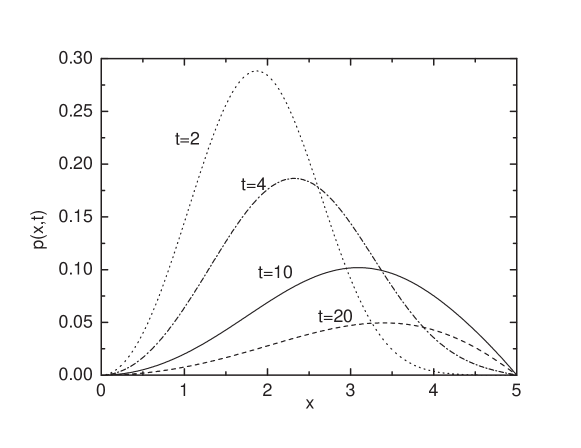
Figure 1: The solutions of Eq.(4) with boundary conditions (11) for $\theta=1$.

Having the distribution $p(x,t)$ calculated, we can determine the survival probability: the probability that the particle is still inside the interval $(0,L)$, i.e. it has not yet reach the absorbing barrier. It can be obtained by means of the formula $S(t)=\int_{0}^{L}p(x,t)dx$ and it determines the first passage time density distribution $f(t)=-dS(t)/dt$. The averaging over that distribution produces the MFPT:

$$T=\int_{0}^{\infty}tf(t)dt=\int_{0}^{L}dx\int_{0}^{\infty}p(x,t)dt.$$ (17)

In the case of our jumping process, the direct evaluation of the integral yields

$$S(t)=\frac{2x_{0}}{\sqrt{L}}\sum_{n}\frac{J_{1/(\theta+2)}\left(\frac{\gamma_{n}}{L^{(\theta+2)/2}}x_{0}^{(\theta+2)/2}\right)}{\gamma_{n}J_{-(\theta+1)/(\theta+2)}(\gamma_{n})}\exp\left(-(\frac{\sigma(\theta+2)}{2\sqrt{2}}\frac{\gamma_{n}}{L^{(\theta+2)/2}})^{2}t\right)$$ (18)

where we utilized simple properties of the Bessel function. To obtain the MFPT we need to integrate $S$ over time:

$$T=\int_{0}^{\infty}S(t)dt=\frac{8x_{0}L^{\theta+3/2}}{\sigma^{2}(\theta+2)}\sum_{n}\frac{J_{1/\theta+2}\left(\frac{\gamma_{n}}{L^{(\theta+2)/2}}x_{0}^{(\theta+2)/2}\right)}{[J^{\prime}_{1/\theta+2}(\gamma_{n})]\gamma_{n}^{3}}.$$ (19)

Fig. 2 presents the survival probability for some values of $\theta$, both positive and negative, calculated from Eq.(18). For the problem without absorbing barriers, the case with $\theta<0$ corresponds to the superdiffusion, whereas with $\theta>0$ – to the subdiffusion. The figure shows that the tails are always exponential. Moreover, $S(t)$ rises with $\theta$ for any $t$, as expected. For large values of $\theta$, beginning of the curve is flat which means that trajectories can hardly escape at short time due to the strong trapping. Since $S(t)$ becomes actually exponential, the MFPT is finite for all $\theta$ (see Eq.(19)), also for those which correspond to the subdiffusion. This result is in contrast to that of the decoupled CTRW which predicts divergence of the MFPT in the subdiffusive case [7]. More precisely, the decoupled CTRW in the subdiffusive case is non-Markovian and it assumes the waiting time distribution in the power law form. Then the mean time of a single jump is infinite. For the problem with the absorbing barriers, one can derive a formula for MFPT directly from the waiting time distribution and the MFPT appears infinite. For the process presented in this paper, the waiting time distribution is exponential and the subdiffusion results from the $x-$dependence of its coefficient, i.e. from nonhomogeneity of the medium. Introduction of that dependence has important physical implications. As regards the application to the heat conduction problem, the subdiffusive thermal conductivity becomes possible also for the systems which are not perfect thermal insulators and then more realistic.

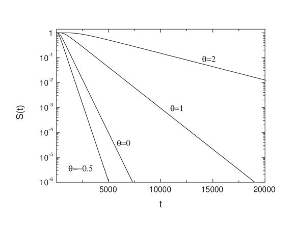
Figure 2: The survival probability calculated from Eq.(18) for the values of $\theta$ which corresponds to the superdiffusion ($\theta<0$), normal diffusion ($\theta=0$), and subdiffusion ($\theta>0$).

4 Lévy flights between the absorbing barriers

In this section we analyse the jumping process for the system restricted by two absorbing barriers for which the jumping size distribution is given by the Lévy distribution. We calculate the probability density distributions and the MFPT as a function of both the Lévy index $\mu$ and the parameter $\theta$.

The MFPT problem for the Lévy flights on the bounded domain, both with and without a potential, is studied extensively in recent years; beside the MFPT, the first passage time distribution has been evaluated as a function of the parameters of the Lévy distribution, which, in general, can be asymmetric. Since the analytical approach is very difficult in this case, most of the studies rely on the Monte Carlo simulations [22, 23, 24]. Nevertheless, recently an analytical solution to the fractional equation with the boundary conditions, which describes the Lévy flights in a homogeneous medium ($\theta=0$), has been found [25].

The Lévy distribution represents the general stable distribution and in that sense it is a generalization of the Gaussian. It accounts for processes for which the second moment of the probability density distribution diverges: the standard central limit theorem does not apply in this case. Phenomena which exhibit distributions with long tails are frequently encountered in nature. They are typical for systems of high complexity, in particular biological [26], social, and financial ones. Therefore, the theory of the Lévy flights is widely applicable to problems from various branches of science and technology.

One can expect that presence of the barriers will influence the stochastic dynamics particularly strong in the case of the Lévy processes. If the interval length $L$ is small compared to the width parameter $\sigma$ of the jump length distribution, the power-law tails of the distribution will not manifest themselves. In particular, all moments become finite.

We assume the jump length distribution in the form

$$Q(x)=\sqrt{2/\pi}\int_{0}^{\infty}\exp(-\sigma^{\mu}k^{\mu})\cos(kx)dk,$$ (20)

as well as the Poissonian waiting time distribution (1). We determine the probability density distribution $p(x,t)$ by means of the Monte Carlo method. The Lévy-distributed jump-size density has been generated by using the algorithm from Ref. [27]. The time evolution of individual trajectories, which start with the same initial condition, has been performed by sampling consecutive values of the jumping size and the waiting time interval from the densities $Q(x)$ and $P_{P}(t)$, respectively. The final results have been obtained by averaging over those individual trajectories. Fig.3 presents the time evolution of $p(x,t)$ for both positive and negative $\theta$. Similarly as in the case of the Fokker-Planck equation, the distributions terminate abruptly at the barrier position and they shrink with time due to the absorption. The initial delta function at $x=2$ is visible up to a long time.

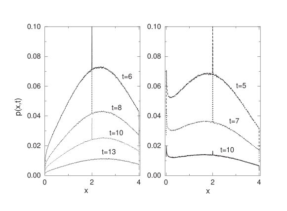
Figure 3: The time evolution of probability density distribution for $Q(x)$ in the form of the Lévy distribution (20) with the parameters $\mu=1.5$ and $\sigma=1$, calculated for two values of $\theta$: $\theta=0.2$ (left part) and $\theta=-0.1$ (right part). The vertical lines near the absorbing barrier $x=4$ represent very fast fall of the distributions due to absorption.

In the case of the process presented in Fig.3 the width parameter $\sigma$ of the driving distribution $Q(x)$ is large, compared to the interval size $L$, and the results are not sensitive to its tails. On the other hand, in the limit of large $\bar{L}=L/\sigma$ one can expect that $p(x,t)$ converges to the distribution which corresponds to the process without absorbing barriers. In this case, the resulting distribution should not depend on $\sigma$ and the asymptotics should be completely determined by $\mu$. Indeed, Fig.4 demonstrates that for $\sigma=0.003$ the tail approaches the form $\sim x^{-1-\mu}$, before it is cut abruptly at the barrier position. For the slightly larger value of this parameter, $\sigma=0.004$, the power-law asymptotics fails to appear. The tails of $p(x,t)$ become $\sigma$-dependent for relatively large $\sigma$ because the importance of the tails of $Q(x)$ gradually declines with $\sigma$.

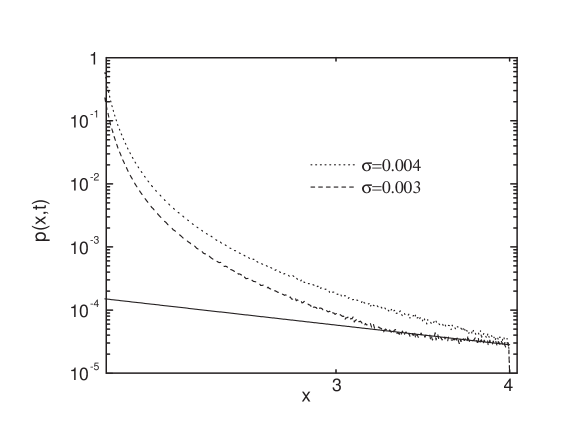
Figure 4: The log-log plot of the tails of probability density distribution $p(x,t)$, calculated with $\theta=0.2$ and $\mu=1.5$, for two values of the width parameter $\sigma$. The solid line denotes the function $\sim x^{-5/2}$.

The same procedure allows us to determine MFPT: the average time $T$ the edge of the interval, i.e. either 0 or $L$, is reached. The dependence of MFPT on both $\mu$ and $\sigma$ is presented in Fig.5 for the case $\theta=0$. In general, $T$ rises with $\mu$ because then the probability of large jumps falls. Since that effect results from the power-law tails, it is weak (the curves are flat) if only the central part of the distribution – similar for all $\mu$ – is involved, i.e. for large $\sigma$. On the other hand, small values of $\sigma$ result in a strong dependence $T(\mu)$, which becomes exponential for $\sigma=0.003$. This shape persists for even smaller $\sigma$.

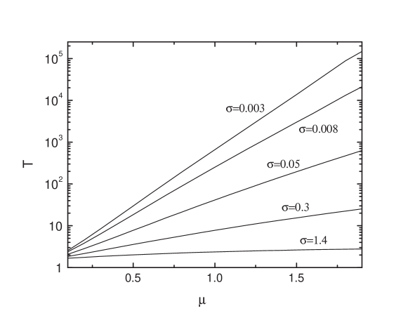
Figure 5: The MFPT as a function of the parameter $\mu$ calculated for $\theta=0$ and some values of $\sigma$.

The parameter $\theta$ is crucial to the speed of the transport; in absence of the absorbing barriers, the cases with large values of $\theta$ correspond to the slow diffusion. It happens because the traps at large distances becomes more effective when $\theta$ increases and the transport is hampered due to the long waiting times. Consequently, one can expect that the MFPT will rise with $\theta$. This conclusion is illustrated in Fig.6. Growth of the function $T(\theta)$ is especially pronounced for large values of $\mu$ (close to Gaussian case $\mu=2$) because then the average jump length is relatively small and a large number of jumps is needed to reach the barrier. Transition from the negative to positive values of $\theta$ – which corresponds to the change of kind of diffusion in the problem without absorbing barriers – is smooth for all $\mu$. The latter conclusion holds also for $\mu=2$, according to the Eq.(19).

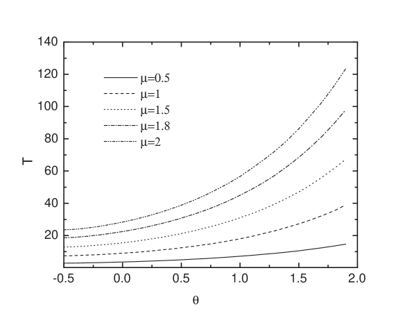
Figure 6: The MFPT as a function of the parameter $\theta$, calculated with $\sigma=0.3$, for some values of $\mu$.

5 Summary and discussion

We have analysed the one-dimensional, step-wise jumping process which is defined on the finite interval, bounded by two absorbing barriers. Since the waiting time distribution involves the variable, position-dependent coefficient, the inhomogeneity of the medium has been taken into account. That, power-law, dependence is a reason of the anomalous behaviour: the diffusion can be both weaker and stronger than normal. The calculated MFPT is large for the subdiffusion and rises with the parameter $\theta$, nevertheless it always assumes a finite value. Physical reason behind the latter outcome – which can never be concluded from the traditional, uncoupled CTRW models of the subdiffusion – is the weakening of trapping with the increased distance and, as a result, the effective mean waiting time is finite. From the point of view of modelling of the anomalous heat conduction, the introduction of the $x$-dependent waiting time distribution allows us to describe the subdiffusive heat transport for realistic systems: for those which are not perfect insulators.

Restrictions imposed on the system by the existence of the absorbing barriers are pronounced if we allow for long jumps, i.e. if the jumping size distribution $Q(x)$ is of the Lévy form. The power law tails of that distribution can influence the probability density distribution of the process, $p(x,t)$, only if $Q(x)$ is narrow, compared to the distance between the barriers, i.e. to the system size. In that limit, the sections of $p(x,t)$ which are close to the barrier assume the power law shape in the same form as the tails for the problem without the barriers. Conversely, for the broad $Q(x)$ those tails are hardly visible and the MFPT is almost independent of the Lévy parameter $\mu$. The dependence of MFPT on the parameter $\theta$ is similar to that for the Gaussian $Q(x)$: large values of $\theta$, for which the transport is strongly hampered by the traps, result in large $T$. Nevertheless, it remains finite, for any $\mu$ and $\theta$.

References

- [1] C. Escudero, J. Buceta, F. J. de la Rubia, and Katja Lindenberg, Phys. Rev. E 69, 021908 (2004).
- [2] G. Abramson and V. M. Kenkre, Phys. Rev. E 66, 011912 (2002).
- [3] H. Risken, The Fokker-Planck Equation (Springer-Verlag, Berlin, 1996).
- [4] S. Lepri, R. Livi, and A. Politi, Phys. Rev. Lett. 78, 1896 (1997).
- [5] S. Denisov, J. Klafter, and M. Urbakh, Phys. Rev. Lett. 91, 194301 (2003).
- [6] P. Cipriani, S. Denisov, and A. Politi, Phys. Rev. Lett. 94, 244301 (2005).
- [7] S. B. Yuste and Katja Lindenberg, Phys. Rev. E 69, 033101 (2004).
- [8] R. Metzler, W. G. Glöckle, and T. F. Nonnenmacher, Physica A 211, 13 (1994).
- [9] R. Metzler and T. F. Nonnenmacher, J. Phys. A 30, 1089 (1997).
- [10] V. E. Tarasov, Chaos 15, 023102 (2005).
- [11] J.-P. Bouchaud and A. Georges, Phys. Rep. 195, 12 (1990).
- [12] S. Lepri, R. Livi, and A. Politi, Phys. Rep. 377, 1 (2003).
- [13] Kwok Sau Fa and E. K. Lenzi, Phys. Rev. E 71, 012101 (2005).
- [14] A. Kamińska and T. Srokowski, Phys. Rev. E 69, 062103 (2004).
- [15] B. O’Shaughnessy and I. Procaccia, Phys. Rev. Lett. 54, 455 (1985).
- [16] A. A. Vedenov, Rev. Plasma Phys. 3, 229 (1967).
- [17] H. Fujisaka, S. Grossmann, and S. Thomae, Z. Naturforsch. Teil A 40, 867 (1985).
- [18] V. M. Zolotarev, One-dimensional Stable Distribution (American Mathematical Society 1986).
- [19] T. Srokowski and A. Kamińska, Phys. Rev. E 74, 021103 (2006).
- [20] T. Srokowski, Phys. Rev. E 75, 051105 (2007).
- [21] E. Kamke, Differentialgleichungen, Lösungsmethoden und Lösungen, Band I (Geest&Portig K.-G., Leipzig, 1956).
- [22] B. Dybiec, E. Gudowska-Nowak and P. Hänggi, Phys. Rev. E 73, 046104 (2006).
- [23] M. Ferraro and L. Zaninetti, Phys. Rev. E 73, 057102 (2006).
- [24] S. L. A. de Queiroz, Phys. Rev. E 71, 016134 (2005).
- [25] A. Zoia, A. Rosso and M. Kardar Phys. Rev. E 76, 021116 (2007).
- [26] B. J. West and W. Deering, Phys. Rep. 246, 1 (1994).
- [27] J. M. Chambers, C. L. Mallows and B. W. Stuck, J. Am. Stat. Assoc. 82, 704 (1987)