On the dynamics of a twisted disc immersed in a radiation field

Abstract

We study the dynamics of a twisted tilted disc under the influence of an external radiation field. Assuming the effect of absorption and reemission/scattering is that a pressure is applied to the disc surface where the local optical depth is of order unity, we determine the response of the vertical structure and the influence it has on the possibility of instability to warping.

We derive a pair of equations describing the evolution of a small tilt as a function of radius in the small amplitude regime that applies to both the diffusive and bending wave regimes. We also study the non linear vertical response of the disc numerically using an analogous one dimensional slab model. For global warps, we find that in order for the disc vertical structure to respond as a quasi uniform shift or tilt, as has been assumed in previous work, the product of the ratio of the external radiation momentum flux to the local disc mid plane pressure, where it is absorbed, with the disc aspect ratio should be significantly less than unity. Namely, this quantity should be of the order of or smaller than the ratio of the disc gas density corresponding to the layer intercepting radiation to the mid plane density, $\lambda\ll 1$.

When this condition is not satisfied the disc surface tends to adjust so that the local normal becomes perpendicular to the radiation propagation direction. In this case dynamical quantities determined by the disc twist and warp tend to oscillate with a large characteristic period $T_{*}\sim\lambda^{-1}T_{K}$, where $T_{K}$ is some ’typical’ orbital period of a gas element in the disc. The possibility of warping instability then becomes significantly reduced.

In addition, when the vertical response is non uniform, the possible production of shocks may lead to an important dissipation mechanism.

1 Introduction

A significant number of X-ray binaries exhibit long-term periodicities on time-scales of  10-100 d. Examples are Her X-1, SS 433 and LMC X-4 see e.g. Clarkson et al. 2003. Precession and warping of a tilted accretion disc has been proposed as an explanation (Katz 1973; Petterson 1975) which has subsequently been found to have observational support (Clarkson et al. 2003). The effect of radiation pressure on a twisted tilted accretion disc was first considered by Petterson 1977a,b who noted that when radiation from the central source is absorbed at the disc surface and re-emitted, a potentially important torque will result. Iping & Petterson 1990 later suggested that such torques determined the shape of the disc and its precession rate. Pringle 1996 subsequently showed that an initially axisymmetric thin disc could be unstable to warping as a result of interaction with an external radiation field (see e.g. Maloney et a. 1998; Ogilvie & Dubus 2001 and Foulkes et al. 2006 for later developments).

The analysis considered the disc to behave as a collection of rings, which could interact by transferring angular momentum through the action of viscosity, but otherwise behaved as if they were rigid. In particular, the vertical displacement or tilt was assumed to be essentially uniform and independent of the vertical coordinate. Thus the pressure applied at the surface at optical depth unity is assumed to be effectively communicated through the disc vertical structure so as to give a near uniform response. In this paper we extend the theoretical treatment of the interaction of a disc with an external radiation field to take account of possible significant departures of the tilt or displacement from uniformity in the vertical direction. One of our objectives is to determine the conditions under which the assumption of a uniform response is valid, and then to estimate some of the consequences when they are not satisfied, including potential additional dissipation resulting from non linear effects such as the production of shock waves. The latter is done using a one dimensional slab analogue model with the required high resolution in the vertical direction.

Although we focus on the effects of a surface pressure induced by an external radiation field, very similar considerations are likely to apply when warps are induced by a surface pressure resulting from interaction with an external wind (e.g. Quillen, 2001) or surface forces produced by the interaction of the disc with an external magnetic field originating in the central star ( e.g. Pfeiffer & Lai, 2004).

We begin by considering the relevant issues using simple physical arguments. Following Pringle 1996 we consider a thin disc immersed in an external radiation field with mid plane initially coinciding with a Cartesian $(x,y)$ plane. It is supposed that the upper surface is parallel to the external rays so that there is initially no interaction with the radiation. The upper surface is then given a vertical elevation $h(r,\phi),$ where we now use polar coordinates $(r,\phi).$ As a result, a disc element with surface area $d{\cal A}$ absorbs momentum from the radiation field at a rate

$${\dot{\cal F}}=F_{0}d{\cal A}\left(r{\partial(h/r)\over\partial r}\right).$$ (1)

Here $F_{0}$ is the momentum flux at radius $r$ associated with the external radiation field. The factor in brackets gives the angle through which the local normal is rotated as a result of the perturbation (see Appendix A for more details). Assuming the absorbed momentum is reradiated isotropically above the disc by the surface layers at an optical depth of unity, there will be an applied pressure there of magnitude

$${\cal P}={2F_{0}\over 3}\left(r{\partial(h/r)\over\partial r}\right).$$ (2)

This external pressure, when applied to a complete elementary ring, produces a net torque per unit length of magnitude

$${d{\cal T}\over dr}={2\pi F_{0}\over 3}\left(r^{2}{\partial(h/r)\over\partial r}\right){\bf l},$$ (3)

where the complex vector ${\bf l}$ has components equal to $(i,1,0)$ in the Cartesian coordinate system. Here, in performing the azimuthal integration, we take into account that the azimuthal dependence of $h$ is through a factor of the form $\exp(-i\phi)$ and work with the radial amplitude from now on.

To find the consequent evolution of the disc, one requires the component of the angular momentum per unit length perpendicular to its unperturbed direction. This is given by

$${d{\cal J}/dr}=2\pi\Sigma r^{2}\Omega{\langle h\rangle}i{\bf l},$$ (4)

with $\Omega$ and $\Sigma$ being the near Keplerian local disc angular velocity and the disc surface density, respectively. $\langle h\rangle=\int d\zeta\rho h/\Sigma$ where $\zeta$ is a vertical coordinate and $\rho$ is the gas density.

For an elementary ring the condition that the rate of change of angular momentum equal the applied torque gives a tilt evolution equation of the form

$${\partial{\langle h\rangle}\over\partial t}=-i{F_{0}\over 3\Omega\Sigma}\left({\partial(h/r)\over\partial r}\right).$$ (5)

Assuming the vertical response is uniform, so that we can set $h={\langle h\rangle}\equiv r{\bf W}$, we obtain a description of warp evolution equivalent to Pringle 1996 when effects due to viscosity and bending wave propagation are neglected (see sections 5.1 and 6.5 below). This description indicates the possibility of instability to radiation pressure warping.

However, here we stress the fact that the averaged elevation $\langle h\rangle,$ enclosed in angled brackets, applies to the bulk of the inertia of the disc and can therefore be shown to be close to the elevation of the mid plane. On the other hand $h$ as used in the torque formula applies to the disc surface elevation. An important aspect of this paper is to distinguish these two elevations and investigate under what conditions they can be taken to be equal. This would be possible if the vertical structure responds as a rigid body to the external pressure forcing and we find the conditions for this to occur. The general requirement is found to be that the density at the surface of the disc where the pressure is applied should not be too small.

It is possible to estimate in a simple way when the vertical displacement response of the disc to the external pressure forcing becomes non uniform. Let us suppose that the external pressure ${\cal P}$ is applied at the surface layer where the density $\rho=\rho_{*}.$ The induced vertical displacement $h,$ now should be considered to be also a function of the vertical coordinate $\zeta.$

Assuming a linear response, which should be appropriate for sufficiently small elevations and, for simplicity an isothermal equation of state with sound speed $c_{s},$ it can be easily shown that in the upper layers of the disc where vertical motions dominate the Lagrangian pressure perturbation has the form determined by presence of $h$, $\Delta P=-\rho_{*}c_{s}^{2}{\partial h\over\partial\zeta}$, see equation (40) below. Equating this to the external pressure we have

$${\partial h\over\partial\zeta}=-{{\cal P}\over\rho_{*}c_{s}^{2}}.$$ (6)

If the vertical extent of the disc is $\zeta_{0},$ and $h$ varies on a radial scale comparable to $r,$ the characteristic change in $h$ induced over the vertical thickness is easily estimated to be

$$\Delta h\sim\zeta_{0}{{\cal P}\over\rho_{*}c_{s}^{2}}\sim{2F_{0}r\over 3\rho_{*}\Omega^{2}\zeta_{0}}\left({\partial(h/r)\over\partial r}\right),$$ (7)

where we use the approximate relation $c_{s}=\Omega\zeta_{0}.$

From the condition $\Delta h\sim h$, using (7) and estimating ${\partial h\over\partial r}\sim h/r$, it is clear that whether $h$ is uniform or not is governed by the the parameter $F_{0}r/(\rho_{*}\Omega^{2}\zeta_{0}^{3})(\zeta_{0}/r)^{2}=\lambda^{-1}\epsilon\delta^{2},$ with $\lambda=\rho_{*}/\rho_{c}$ and $\delta=\zeta_{0}/r$ so defining $\epsilon=F_{0}r/(\rho_{c}\Omega^{2}\zeta_{0}^{3}).$

For a uniform response, one requires that $\epsilon\delta^{2}\ll\lambda.$ This is equivalent to the requirement that the product of the ratio of the external radiation momentum flux to the local disc pressure with the disc aspect ratio should be significantly less than unity. We recall here that because of the geometrical configuration, the momentum flux locally reradiated by the disc is in general much less than the external momentum flux at that location.

In this paper we extend the treatment of disc warping induced by the action of an external pressure to include the effects of the response of the vertical structure particularly when this is non uniform as is the case when the above condition is not satisfied. In that case we find that the disc dynamics enters a different regime. This is such that the exposed surface tends to align so as to reduce the momentum absorption and hence the applied pressure. In the extreme limit of this regime the upper surface acts as if it is in contact with a rigid wall with the tendency to radiation warping instability tending to vanish. In this limit quantities characterising the disc twist and warp tend to oscillate at typical frequency $\sim\lambda\Omega$.

To illustrate these effects we derive a description of the one dimensional evolution of the disc inclination in radius and time that incorporates the effects of the vertical structure response, radiation torques and which applies both to the high viscosity regime, when the evolution is diffusive, and to the low viscosity regime when the evolution is wavelike. In all cases, the efficacy of surface radiation pressure driven instabilities is found to be reduced once the model parameters are such that the vertical response is significantly non uniform.

We go on to estimate conditions for the response to be nonlinear and investigate the development of shock waves in the response using a one dimensional slab analogue model which has the same characteristic behaviour of linear perturbations as the full disc model. We find that such shocks potentially provide an important dissipation mechanism.

The plan of this paper is as follows. In section 2 we describe some aspects of the thin disc model used. In section 3 we go on to introduce the twisted coordinate system used together with the notation convention, giving the basic equations in section 4. By integrating over the vertical direction we use these to derive a single equation governing the dynamics of a twisted disc in section 5. When the disc behaves like a set of rigid rings for which the vertical response is uniform, this equation can be used to give a complete specification of the warp evolution. We note that this provides an extension of previous formulations to be able to consider the case when warps propagate as waves rather than diffuse radially (e.g. Nelson & Papaloizou 1999).

In this Paper we use the twisted coordinate system formalism first introduced by Petterson 1977a, 1978 where the dynamical equations take the most simple form. When this formalism is adopted and an accurate description of all components of the equations of motion is needed as in the problem on hand we show that, in general, there is an ambiguity in choice of twisted coordinates with a set of these describing the same physical situation. As discussed in section 5 a choice of a most appropriate twisted coordinate system can be motivated by the condition that perturbations of all dynamical quantities determined by the disc twist and warp are small. The transformation law between different twisted coordinates corresponding to the same physical situation is derived in appendix C for an inviscid disc.

In order to obtain a complete description of the warp evolution when the vertical response is non uniform, we begin by obtaining a complete solution of the vertical problem for a polytropic model in section 6.1. This is used to obtain a pair of equations governing the radial warp evolution. We also indicate how the results can be extended to apply to more general models. We confirm the condition for the disc response to be like that of a series of rigid rings as $\lambda\gg\epsilon(\zeta_{0}/r)^{2}.$

We go on to perform a linear stability analysis of the radial evolution equations adopting a WKB approach in section 7 obtaining a maximum potential growth/decay rate in section 7.3. In section 8 we discuss and confirm the analogy between the response of the disc and the linear and non linear dynamics of a vertically stratified one dimensional slab. We consider the development of shock waves and the formation of a rarefied hot atmosphere in section 8.3 giving a crude estimate of the warp dissipation rate in section 8.4. Finally in section 9 we discuss and summarize our results.

2 A thin disc model

To begin we briefly summarize some of the properties of an unperturbed axisymmetric thin accretion disc model which are used in the discussion below.

However, the physical basis of our results does not depend on the detailed properties of this model which has been used for the purpose of making specific calculations. In order to make our treatment as simple as possible we use a highly simplified version of the Shakura $\&$ Sunyaev 1973 $\alpha$-disc model. We assume a polytropic equation of state for the disc gas

$$P=K(r)\rho^{\gamma}$$ (8)

where $P$ and $\rho$ are the gas pressure and density, $r$ is the radial coordinate and $\gamma$ is the assumed constant specific heat ratio. It is assumed that the ”polytropic constant” $K$ is, in general, a function of the radial coordinate, $r,$ but does not depend on the local vertical coordinate $\zeta$, see equations (14), (15) below for a definition of the coordinate system used in our study. The equilibrium variation of density and pressure with height follows from the equation of state (8) together with the equation of hydrostatic equilibrium

$${\partial P\over\partial\zeta}=c_{s}^{2}{\partial\rho\over\partial\zeta}=-\rho\Omega^{2}\zeta.$$ (9)

Here $c_{s}$ is the adiabatic sound speed, $\Omega=\sqrt{(GM)/r^{3}}$ is the Keplerian angular velocity and $M$ is the mass of a central object.

Integration of equation (9) gives

$$\rho=\rho_{c}(r)\left(1-\left({\zeta\over\zeta_{0}(r)}\right)^{2}\right)^{{1\over 1-\gamma}},\quad P=P_{c}(r)\left(1-\left({\zeta\over\zeta_{0}(r)}\right)^{2}\right)^{{\gamma\over 1-\gamma}},$$

$$\qquad\qquad\qquad\qquad\qquad\qquad c_{s}^{2}=\gamma{P_{c}\over\rho}\left(1-\left({\zeta\over\zeta_{0}(r)}\right)^{2}\right),$$ (10)

where $\rho_{c}$ and $P_{c}$ are the mid plane values of the density and pressure, respectively and $\zeta_{0}$ is the disc semi-thickness. These quantities are related to each other through

$$\Omega^{2}\zeta^{2}_{0}={2\gamma\over\gamma-1}{P_{c}\over\rho_{c}}.$$ (11)

As shown below, many of our equations take an especially simple form for the case $\gamma=5/3,$ accordingly we adopt this value below.

It is assumed below that the standard Navier-Stokes equations are valid as the dynamical equations of our problem with the viscosity law set up according to the standard prescription (Shakura $\&$ Sunyaev 1973 )

$$\nu=\alpha\Omega^{-1}P,$$ (12)

where $\nu$ is the kinematic viscosity. For simplicity we assume below that $\alpha$ is a small constant parameter and consider only leading terms in corresponding expansion series.

The radiation intercepted by the disc is considered to result in an external pressure applied to a surface near to the free surface of the disc. This surface is formally defined through the condition $\rho=\rho_{*}(\tau=1)$ where $\tau$ is the optical depth. It is assumed hereafter that the ratio of the density at this surface to the midplane density $\rho_{*}/\rho_{c}\ll 1$. Thus, we neglect the effect of heating of the upper disc layers by incident radiation. Also, for simplicity it is assumed that the radiation does not affect the structure of the unperturbed disc. This can be achieved by setting the disc semi-thickness to be proportional to the radial distance

$$\zeta_{0}=\delta r,$$ (13)

where $\delta\ll 1$ is the disc opening angle which is constant.

3 Coordinate system and notation convention

The dynamical equations governing a twisted disc take their simplest form in the so-called twisted coordinate system first introduced by Petterson 1977a. Since this system has been discussed extensively elsewhere (for details see e.g. Petterson 1977a; 1978), in this paper we give only some basic definitions and relations important for the future discussion.

In order to define the twisted coordinates let us consider a fixed Cartesian coordinate system $(x_{1},x_{2},x_{3})$ with origin at the central star and $(x_{1},x_{2})$ plane coinciding with the mid-plane of the unperturbed disc. We then perform two elementary rotations of the coordinate axes parametrised by the two Euler angles $\gamma$ and $\beta.$ The first rotation is of the $(x_{1},x_{2})$ axes through the angle $\gamma$ keeping the $x_{3}$ axis fixed. As a result of this rotation the $x_{1}$ and $x_{2}$ axes change their directions. The second rotation is of the $(x_{2},x_{3})$ axes in the plane perpendicular to the new fixed direction of the $x_{1}$ axis and is through the angle $\beta.$ The cylindrical coordinates $(r,\psi,\zeta)$ defined with respect to the rotated axes now determine the twisted coordinate system.

Formally, in the linear approximation that the inclination $\beta$ is small, the transformation to the twisted coordinate system $(r,\psi,\zeta)$ from the initial Cartesian coordinates $(x_{1},x_{2},x_{3})$ is given by

$$\left(\matrix{r\cos\psi\cr r\sin\psi\cr\zeta\cr}\right)=B(\beta,\gamma)\left(\matrix{x_{1}\cr x_{2}\cr x_{3}\cr}\right),$$ (14)

where $B$ is the rotation matrix

$$B(\beta,\gamma)=\left(\matrix{\cos\gamma&\sin\gamma&0\cr-\sin\gamma&\cos\gamma&\beta\cr\beta\sin\gamma&-\beta\cos\gamma&1}\right),$$ (15)

and $\beta(t,r)$ and $\gamma(t,r)$ are, in general, functions of $r$ and the time $t.$

Instead of the original Euler angles it is useful to introduce the combinations $\psi_{1}=\beta\cos\gamma$, $\psi_{2}=\beta\sin\gamma.$ Further, we define the angle $\phi=\psi+\gamma$ which is used to replace the angle $\psi.$ We are thus able to consider the case $\beta(r,t)=0$ for which the transformation (15) is degenerate. The rotation matrix giving the transformation from the twisted coordinates back to the Cartesian coordinates is given by transpose of $B$, $B^{T}$. The cylindrical coordinates $(r_{c},\phi_{c},z_{c})$ associated with the original Cartesian system are defined through: $x_{1}=r_{c}\cos\phi_{c}$, $x_{2}=r_{c}\sin\phi_{c}$ and $x_{3}\equiv z_{c}.$ From equations (14) and (15) we obtain

$$\sin\phi_{c}=\sin\phi-{\beta\zeta\over r}\cos\phi\cos(\phi-\gamma),$$ (16)

$$r_{c}=r-\beta\zeta\sin(\phi-\gamma),$$ (17)

and

$$z_{c}=\zeta+\beta r\sin(\phi-\gamma).$$ (18)

From equations (16) and (17) it follows that when $\zeta=0$ we have $\phi_{c}=\phi$ and $r_{c}=r.$ In addition, the difference $\phi_{c}-\phi$ is also first order in the small angle $\beta.$ Thus we can set $\phi_{c}=\phi$ in equations for quantities that are first order in $\beta.$

All vectors and tensors appearing in our calculations are projected onto a local orthonormal basis ${{\bar{e}}}_{r}$, ${{\bar{e}}}_{\psi}$, and ${{\bar{e}}}_{\zeta}$ (Petterson 1977a, 1978) where the bar is used to denote a vector quantity from now on. The explicit expressions for the above basis vectors are not important for our purposes and can be found elsewhere, see e.g. Petterson 1977a, 1978, Demianski $\&$ Ivanov 1997 hereafter DI. We note, however, that the basis can be uniquely defined by the requirement that ${{\bar{e}}}_{\zeta}$ is the coordinate vector such that ${{\bar{e}}}_{\zeta}\cdot\nabla\equiv{\partial\over\partial\zeta}$ for $\zeta\rightarrow 0.$ All other vectors can be found from the orthonormality conditions together with the requirement that the coordinate axes form a right handed system.

3.1 State variables

Since the coordinate lines of the twisted coordinate system are not orthogonal and both the coordinate lines and directions of the basis vectors depend on time and on the radial coordinate, differentiation of quantities is best performed with help of appropriate connection coefficients. Their explicit form can be found in Petterson 1977a, 1978 and DI. Also, we note that the projections of the velocity vector ${\bar{v}}$ onto the basis vectors are not in general proportional to the time derivatives of the appropriate coordinates of a particular fluid element, see Petterson 1978. Accordingly, we give relations between these components and the time derivative of the appropriate gas element coordinates where this is explicitly needed.

Writing them in the twisted coordinate system, in the approximation that the inclination angle is small enough that a linearization procedure in which quadratic and higher powers of $\beta$ can be neglected, the Navier-Stokes equations and the continuity equation then lead to:

1) a set of equations for unperturbed quantities $Q_{0}$ formally coinciding with the equations describing them for flat disc accretion.

2) A set of equations for quantities $Q_{1}$, which are non axisymmetric perturbations to $Q_{0}$ induced by deformation of the disc shape. The dependence of the latter quantities on $\phi$ is harmonic: $Q_{1}=Q_{1}^{(1)}\cos\phi+Q_{1}^{(2)}\sin\phi$

It is convenient to represent these perturbations as well as the angles $\beta$ and $\gamma$ using the complex quantities, ${\bf Q}$ and ${\bf W},$ which are defined through

$${\bf Q}=Q_{1}^{(1)}+iQ_{1}^{(2)},\quad{\bf W}=\beta e^{i\gamma}=\Psi_{1}+i\Psi_{2}.$$ (19)

Here we note that we adopt the convention that quantities in bold represent complex perturbations. This convention applies also to the components of a vector with vectors themselves denoted with an over bar. When real as in the perturbed equations of motion (23)-(29) given below, these are not in bold. Note also that for convenience we use $\rho_{1}$ and $\xi^{\zeta}$ to denote the complex density perturbation and vertical component of the Lagrangian displacement below, and these are not in bold.

4 Basic equations

As we mentioned above we write each of the variables entering the continuity and the Navier-Stokes equations as the sum of an unperturbed part, formally coinciding with a solution of the equations for axisymmetric thin disc accretion, and a perturbation. Accordingly, we have

$$v^{i}=v_{0}^{i}+v^{i}_{1},\quad\rho=\rho_{0}+\rho_{1},$$ (20)

for the components of velocity and the gas density respectively. But as the only non zero component of the unperturbed velocity is in the azimuthal direction and corresponds to Keplerian rotation which we deal with explicitly, we shall drop the subscript $1$ from the velocity perturbation.

The unperturbed gas density $\rho_{0}$ is given by equation (10). We assume that only circular Keplerian motion of the gas is present in the unperturbed state and accordingly have $v_{0}^{\phi}=r\Omega=\sqrt{{GM\over r}}$. Thus we neglect the radial component of the unperturbed velocity $v_{0}^{r}$ present in the thin disc mainly due to action of viscosity. This can be done in the limit of a sufficiently small value of $\alpha<1$.

Apart from two significant modifications, our equations for the perturbed quantities follow from the corresponding equations given in DI provided that terms involving quadratic and higher order corrections in the assumed small parameter $\alpha$ are discarded and that the gravitomagnetic force in the $\zeta$ component as well as relativistic post-Newtonian corrections to the $r$ and $\phi$-components of the Navier-Stokes equations are neglected.

The most important modification stems from the fact that in the present study an accurate description of vertical motions and displacements is needed and therefore, we take into account all contributions to the vertical velocity, ${v}^{\zeta}.$ These consist of the contribution determined by time-dependent evolution of the basis vector ${\bar{e}}_{\zeta}$ and the contribution determined by time dependent vertical displacements of gas elements in the disc. Accordingly, we have

$${v}^{\zeta}=r{\cal U}+v^{\zeta}.$$ (21)

where ${\cal U}=\dot{\beta}\sin\psi-\beta\dot{\gamma}\cos\psi=\dot{\Psi}_{1}\sin\phi-\dot{\Psi}_{2}\cos\phi$ and the dot stands for the time derivative. The relation of $v^{\zeta}$ to the corresponding component of the displacement vector ${\bar{\xi}},$ $\xi^{\zeta},$ is given by Petterson 1978

$$v^{\zeta}=\dot{\xi}^{\zeta}+\Omega{\partial\over\partial\phi}\xi^{\zeta}.$$ (22)

Only the first term in (21), which arises from the time dependence of the changing coordinate system, is normally taken into account in studies of twisted discs that use the formalism of the twisted coordinate system, see Hatchett at al 1981 and DI. However, the role of the second term, which describes the disc motion relative to the moving coordinates, is essential for our purposes.

We also take into account the time derivative of the perturbed density $\rho_{1}$ in the continuity equation and the time derivative of $v_{\zeta}$ in the $\zeta$-component of the Navier-Stokes equation. These terms are proportional to a small parameter $1/(\Omega t_{ev})$ where $t_{ev}$ is a characteristic evolution time of the twisted disc. That is for any perturbation quantity ${\bf Q},$ we can write $|{\dot{\bf Q}}/{\bf Q}|=O(1/(\Omega t_{ev})).$ However, even though they are small, in a formal sense, when compared with leading terms in a series expansion, when retained, they allow us to regularise some otherwise formally singular expressions, that arise when dealing with the particular problem of calculating the vertical displacements in the disc, see e.g. equation (50) below.

The perturbed Navier-Stokes equations can be divided into ’horizontal’ part incorporating the $(r)$ and $(\phi)$-components and ’vertical’ part corresponding to the $(\zeta)$ component. The horizontal part follows from the equations provided in DI when the relativistic corrections are neglected and the limit of small viscosity is adopted. The $(r)$-component can be written as

$$\rho_{0}(\dot{{{v}}^{r}}+\Omega({\partial\over\partial\phi}{v}^{r}-2{v}^{\phi}))=-\rho_{0}\Omega^{2}r\zeta{\cal W}-{{\partial}\over{\partial\zeta}}t^{r\zeta}.$$ (23)

where ${\cal W}=\beta^{\prime}\sin(\psi)-\beta\gamma^{\prime}\cos\psi=\Psi_{1}^{\prime}\sin\phi-\Psi_{2}^{\prime}\cos\phi$ and

$$t^{r\zeta}=-\eta{{\partial}\over{\partial\zeta}}{v^{r}}$$ (24)

is the $(r,\zeta)$-component of the viscosity tensor. In the expression for ${\cal W},$ a prime denotes differentiation with respect to $r.$

Differentiating the $(\phi)$-component of perturbed Navier-Stokes equations with respect to $(\phi)$ we obtain

$$\rho_{0}{{\partial}\over{\partial\phi}}{\dot{v^{\phi}}}+{\rho_{0}\Omega\over 2}\left({{\partial}\over{\partial\phi}}{v}^{r}-2{v}^{\phi}\right)=-{{\partial^{2}}\over{\partial\zeta\partial\phi}}t^{\zeta\phi},$$ (25)

where

$$t^{\phi\zeta}=-\eta{{\partial}\over{\partial\zeta}}{v}^{\phi}.$$ (26)

The set of equations (21) and (24) can be used in order to express the perturbed velocity components in terms of the quantity $\cal W$. As seen from equations (21) and (24), to the leading order in small parameters $\alpha$ ( or equivalently $\eta$) and $1/(\Omega t_{ev})$, the perturbed velocity components enter in both equations in the same combination

$${{\partial}\over{\partial\phi}}{v}^{r}-2{v}^{\phi}.$$ (27)

Therefore, these equations are degenerate to leading order and accordingly the next order corrections have to be retained (Papaloizou $\&$ Pringle 1983, hereafter PP). This leads to an inverse dependence of the ’horizontal’ part of the perturbed velocity on the small parameters such that both ${v^{r}}$ and ${v^{\phi}}$ are $\propto\min(\alpha^{-1},1/(\Omega t_{ev}))$ (see PP for details).

The $(\zeta)$-component of the Navier-Stokes equation is written in the form

$$\rho_{0}\left(\dot{v}^{\zeta}+\Omega{\partial\over\partial\phi}v^{\zeta}+2\Omega r{\partial\over{\partial\phi}}{\cal U}\right)=-\Omega^{2}\zeta\rho_{1}-{\partial\over\partial\zeta}P_{1},$$ (28)

where $\rho_{1}$ and $P_{1}$ are the perturbations of density and pressure, respectively. These are related through $P_{1}=c_{s}^{2}\rho_{1}$ with the sound speed given by equation (10).

The continuity equation is formally equivalent to perturbed continuity equation written for the case of a flat disc in cylindrical coordinate system

$$\dot{\rho}_{1}+\Omega{\partial\over\partial\phi}\rho_{1}+{{\rho_{0}}\over r}{{\partial}\over{\partial\phi}}{v}^{\phi}+{1\over r}{{\partial}\over{\partial r}}(\rho_{0}{v}^{r}r)+{{\partial}\over{\partial\zeta}}(\rho_{0}v^{\zeta})=0.$$ (29)

We recall that the relation between the velocity component $v^{\zeta}$ and the corresponding component of the Lagrangian displacement vector ${\bar{\xi}}$ is given by equation (22).

Apart from the terms proportional to $\cal W$ and $\cal U$ equations (23-29) are formally equivalent to the corresponding equations that would be written down directly in a fixed cylindrical coordinate system $(r,\phi,\zeta)$ (PP).

The term proportional to $\cal W$ in equation (23) is essentially a projection of the pressure gradient. Due to the presence of perturbations with odd symmetry with respect to $\zeta$ in twisted discs, surfaces of constant pressure do not in general coincide with the orbital planes of gas elements. Therefore, there is is a projection of the pressure gradient onto such an orbital plane which is described by this term, see Fig. 4 of Ivanov $\&$ Illarionov 1997 for graphic representation of this effect.

The term proportional to $2{\partial\over{\partial\phi}}{\cal U}$ in equation (28) is made up from two contributions. The first is related to the non-holonomic character of our basis vectors. As we have mentioned above in a non-stationary situation, this leads to a non-zero vertical velocity even for a gas element being at rest with respect to the twisted coordinate system, see equation (21) above. This fact was noted for the first time by Hatchett, Begelman $\&$ Sarazin 1981. The second contribution is determined by non-inertial effects. These are taken into account by an appropriate connection coefficient in the formalism developed by Petterson 1978. Both contributions have exactly the same form. This accounts for the factor $2$ in the expression $2{\partial\over{\partial\phi}}{\cal U}$ in equation (28).

The set of equations (23-29) can be brought into a simpler form with help of the complex notation introduced through equation (19) for the density perturbation and the perturbations to the velocity components. Also, we assume hereafter that all perturbed quantities depend on $\phi$ and time only through an exponential factor. Thus

$${\bf Q}\propto e^{-i\omega t-i\phi},$$ (30)

where the frequency $\omega$ is, in general, a complex constant.

Subtracting equation (25) from equation (23) and introducing the complex notation it is easy to see that the result contains the components of the velocity perturbation only in the combination ${\bf v}_{+}={{\bf v}}^{r}+2i{{\bf v}}^{\phi}$. The resulting equation can thus be represented as

$$i\omega\rho{\bf v}^{+}+{\partial\over\partial\zeta}\eta{\partial\over\partial\zeta}{\bf v}^{+}=i\rho\Omega^{2}r\zeta{\partial{\bf W}\over\partial r},$$ (31)

where we use equations (24) and (26) and set $\rho\equiv\rho_{0}$ from now on. The quantities ${{\bf v}}^{r}$ and ${{\bf v}}^{\phi}$ can be separately expressed in terms of ${\bf v}_{+}$ taking into account the fact that in the leading approximation in the small parameters we can equate expression (27) to zero and, accordingly, obtain

$${{\bf v}}^{r}-2i{{\bf v}}^{\phi}=0,\quad{{\bf v}}^{r}={1\over 2}{\bf v}^{+},\quad{{\bf v}}^{\phi}=-{i\over 4}{\bf v}^{+}.$$ (32)

Now we can express ${{\bf v}}^{r}$ and ${{\bf v}}^{\phi}$ in terms of ${\bf W}$ with help of equations (31) and (32). To do this we remark that the $\zeta$ dependence is dealt with by noting that $\eta\propto P$ and the solution is such that both ${{\bf v}}^{r}$ and ${{\bf v}}^{\phi}$ are $\propto\zeta.$ We then use the resulting expressions to eliminate these velocity components in the continuity equation (29) so obtaining

$$(\omega+\Omega){\bf\rho}_{1}=-i\left(\rho{\bf A}\zeta+{{\partial}\over{\partial\zeta}}(\rho{\bf v}^{\zeta})\right),$$ (33)

where

$${\bf A}={GM\over r^{1/2}}\rho^{-1}{{\partial}\over{\partial r}}\left({\rho r^{-3/2}\over{\hat{\omega}}}{\partial{\bf W}\over\partial r}\right),$$ (34)

and

$$\hat{\omega}=\omega+i\alpha\Omega.$$ (35)

Finally, equations (28) and (22) can be brought in the form

$$-i\rho(\omega+\Omega){\bf v}^{\zeta}=2i\rho\Omega\omega r{\bf W}-\Omega^{2}\zeta{\bf\rho}_{1}-{{\partial}\over{\partial\zeta}}c_{s}^{2}{\bf\rho}_{1},$$ (36)

and

$${\bf v}^{\zeta}=-i(\omega+\Omega){\bf\xi}^{\zeta}.$$ (37)

5 Derivation of a single equation describing the dynamics of a twisted disc

At first let us point out that the hydrodynamical equations as written in a twisted coordinate system cannot in principle provide a single dynamical equation for ${\bf W}$ without some additional considerations. Indeed, since the Euler angles $\beta$ and $\gamma$ are considered as dynamical variables in this formalism, the total number of dynamical variables is always larger by two than the number of equations actually needed to determine the dynamics of the system.

For example, in the case of a baratropic equation of state $P=P(\rho),$ there are six dynamical variables used in the description of the problem, these being the three components of velocity, and the density together with the two Euler angles. However the number of dynamical equations available is four, these being the three components of the Navier-Stokes equations, and the continuity equation. Since the number of equations is smaller than the number of variables, there are in principal, different sets of variables ${\bar{v}}(t,r)$, $\rho_{1}(t,r)$ and ${\bf W}(t,r)$ describing the same dynamical system and connected to each other by certain transformation laws. These transformation laws can be easily found from the condition that the velocity and density fields measured in some inertial coordinate system remain unchanged when the set of dynamical variables associated with the twisted coordinate system is transformed. Explicit expressions for these transformation laws are given in Appendix C. It is interesting to note that the dynamical variables in the inertial coordinate system play the role of gauge independent quantities and the laws of transformation between different sets of variables in the twisted coordinate system may be regarded as gauge transformations. This situation has many analogies in different physical systems, say in systems governed by General Relativity, such as e.g. , the theory of small cosmological perturbations, see e.g. Landau $\&$ Lifshitz 1975.

In order to begin the process of obtaining a single equation describing the dynamics of a twisted disc referred hereafter as a ’dynamical equation’ we substitute the density perturbation given by equation (33) into the ’vertical’ equation (36) thus having

$${{\partial}\over{\partial\zeta}}\left(c_{s}^{2}\rho_{0}{{\partial}\over{\partial\zeta}}{\bf v}^{\zeta}\right)+2\rho_{0}\Omega\omega{\bf v}^{\zeta}=-2\rho_{0}\Omega^{2}\omega r{\bf W}-\rho_{0}\Omega^{2}{\bf A}\zeta^{2}-{{\partial}\over{\partial\zeta}}(c_{s}^{2}\rho_{0}{\bf A}\zeta),$$ (38)

where we use the hydrostatic balance equation (9) and approximate $\Omega+\omega\approx\Omega$ in the first term on the right hand side. Equation (38) plays an important role in our analysis. A dynamical equation follows from (38) provided that appropriate boundary conditions at the disc surface are specified.

5.1 A simple approach to the derivation of a dynamical equation

Before discussing an approach to the problem which fully takes into account the vertical structure of the disc, we would like to show how to obtain a governing dynamical equation from equation (38) in a straightforward way. Although this approach is incomplete it allows us to obtain a dynamical equation which is approximately correct provided that the ratio of the density where the external pressure is applied to the central density, $\lambda=\rho_{*}/\rho_{c}$, is not too small.

To do this we integrate equation (38) over $\zeta$ taking into account the fact that the last term on the right hand side vanishes when $\zeta\rightarrow\pm\zeta_{0}$ and can be discarded. We thus obtain

$$\left(c_{s}^{2}\rho{{\partial}\over{\partial\zeta}}{\bf v}^{\zeta}+c_{s}^{2}\rho{\bf A}\zeta\right){\huge|}^{\zeta\rightarrow\zeta_{0}}_{\zeta\rightarrow-\zeta_{0}}+2\Omega\omega\int^{+\zeta}_{-\zeta}\rho{\bf v}^{\zeta}d\zeta=$$

$$\qquad\qquad\qquad\qquad\qquad-2\Sigma\Omega^{2}\omega r{\bf W}-{GM\Omega^{2}\over 2r^{1/2}}{{d}\over{dr}}\left({\Sigma H^{2}r^{-3/2}\over\hat{\omega}}{{d}\over{dr}}{\bf W}\right),$$ (39)

where $\Sigma=\int^{+\zeta_{0}}_{-\zeta_{0}}d\xi\rho_{0}$ is the surface density and a typical disc height $H$ is defined by condition $H^{2}=\int^{+\zeta_{0}}_{-\zeta_{0}}d\zeta\zeta^{2}\rho_{0}/\Sigma$.

It can be easily shown that the surface terms on the left hand side are, in the low frequency limit, proportional to the Lagrangian pressure perturbation, $\Delta P=(dP_{0}/d\zeta)\xi^{\zeta}+P_{1}$. Introducing the complex notation and taking into account that in the low frequency limit, we can write from (37) that ${\bf\xi}^{\zeta}\approx i\Omega^{-1}{\bf v}^{\zeta},$ we obtain

$$\Delta{\bf P}\approx i{dP_{0}\over d\zeta}\Omega^{-1}{\bf v}^{\zeta}+c_{s}^{2}{\bf\rho}_{1}\approx-i\Omega^{-1}\left(c_{s}^{2}\rho{{\partial}\over{\partial\zeta}}{\bf v}^{\zeta}+c_{s}^{2}\rho{\bf A}\zeta\right),$$ (40)

where we make use of equation (33) and use the hydrostatic balance condition (9).

The Lagrangian pressure perturbation must be equal to the radiation pressure at the surface corresponding to an optical thickness expected to be of order unity. As we discuss in Appendix A we can assume that the radiation pressure acts only on the upper surface of the disc ( i.e. where $\zeta\rightarrow+\zeta_{0}$). We set, accordingly, the surface term corresponding to the lower surface of the disc to zero, and express the term corresponding to the upper surface in equation (39) with help of equation (40) through the radiation pressure term ${\bf F}_{+}$ given by equation (109) of Appendix A to obtain

$$\omega r{\bf W}+{F_{0}\over 3\Sigma\Omega}{d\over dr}(i{\bf\xi}^{\zeta}/r-{\bf W})+{GM\over 4\Sigma r^{1/2}}{{d}\over{dr}}\left({\Sigma H^{2}r^{-3/2}\over\hat{\omega}}{{d}\over{dr}}{\bf W}\right)=0,$$ (41)

where we neglect the second term of the left hand side of (39) proportional to $\omega$ in order to get (41). This procedure is justified below, see Section 6.4 where we derive a similar equation in a more rigorous way.

Also, let us stress that the $(\zeta)$-component of the displacement vector is assumed to be evaluated at the surface of the unperturbed disc where the optical thickness $\tau$ is of the order of unity, and let us recall that $F_{0}$ is the radiation momentum flux per unit area perpendicular to the radial direction, see Pringle 1996.

The density $\rho_{*}(\tau\approx 1)$ where the external radiation pressure is applied, is assumed to be always much smaller than the mid plane density $\rho_{c}$.

We comment that in the absence of radiation pressure, equation (41) describes the linear dynamics of a free warped disc. When $\alpha=0,$ this is wavelike, the waves being non dispersive and having local speed $\Omega H/2$, see Nelson & Papaloizou 1999, Papaloizou & Lin 1995, Nelson & Papaloizou 2000. Furthermore we comment, without giving details, that equation (41) may also be derived following the approach discussed in those papers, so confirming the analysis based on the adoption of a twisted coordinate system presented here.

The radiation pressure term involves the combination ${\bf\xi}^{\zeta}/r+i{\bf W}.$ This can be regarded as being the angular displacement of the surface of the disc. It is composed of two parts. The first $\xi^{\zeta}/r$ represents the displacement of the surface of the disc relative to the midplane. The second term $i{\bf W}$ can be viewed as representing the displacement of the midplane and is described by the twisted coordinate system. When the disc behaves like a rigid ring, the contribution of ${\bf\xi}^{\zeta}$ is small.

5.2 The small parameter $\lambda=\rho_{*}/\rho_{c}$

The small parameter $\lambda=\rho_{*}/\rho_{c}$ should be compared with other small parameters of the problem in order to specify the different possible regimes of dynamical evolution of the disc. In particular, as we show below it is important to compare it with the local growth rate, in units of $\Omega,$ associated with any possible instability of the disc that is driven by radiation pressure, ${\tilde{\omega}}_{r}.$

As mentioned in the introduction and elaborated further below, we will see, when $\lambda>{\tilde{\omega}}_{r},$ we can neglect ${\bf\xi}^{\zeta}$ in the expression ${\bf\xi}^{\zeta}/r+i{\bf W}$ entering in (41). Physically this corresponds a situation when the surfaces of constant density in the disc are approximately parallel to each other and remain at an approximately constant distance apart. In that case, for the purpose of calculation of the radiation pressure term, the disc may be considered as being composed of rigid rings having different inclinations and precession angles and the analysis undertaken in previous studies (e.g. Pringle 1996) applies. Neglecting the displacement ${\bf\xi}^{\zeta}$ in (41), we see that this equation gives the evolution of ${\bf W}$ without the need for additional considerations. For the case $\alpha>\delta$ the frequency $\omega$ may be neglected in the expression $\hat{\omega}=\omega+i\alpha\Omega$ and equation is reduced to a form analogous to that obtained by Pringle 1996. In this case Pringle 1996 indicated that the disc may be unstable in linear theory provided that the radiation pressure term is sufficiently large.

In the opposite limit $\delta>\alpha,$ equation (41) describes wave-like propagation of twisted disturbances of the disc (see Nelson & Papaloizou 1999, Papaloizou & Lin 1995, Nelson & Papaloizou 2000) as indicated above, modified by the presence of the radiation pressure term.

5.3 The polytropic model and the dynamical equation in a ’standard’ form

For the polytropic equation of state we can bring equation (41) to a further reduced form. In this case one can obtain from equation (10)

$$\Sigma=\sqrt{\pi}({\Gamma({\gamma\over\gamma-1})\over\Gamma({\gamma\over\gamma-1}+{1\over 2})})\rho_{c}\zeta_{0},\quad H^{2}={(\gamma-1)\over(3\gamma-1)}\zeta_{0}^{2},$$ (42)

where $\Gamma(x)$ is the gamma function.

Before derivation of the general dynamical equation let us now temporary assume that the disc parameters are such that $\lambda>\delta^{2}/\alpha$ and the term proportional to ${\bf\xi}^{\zeta}$ in (41) can be neglected and obtain an equation analogous to what has been obtained by Pringle (1996) for the polytropic model. In this case we can use equation (42) and rewrite equation (41) in the form

$$\omega r{\bf W}-{\Gamma({\gamma\over\gamma-1}+{1\over 2})\over 3\sqrt{\pi}\Gamma({\gamma\over\gamma-1})}\zeta_{0}\tilde{F}_{0}{{d}\over{dr}}{\bf W}+{(\gamma-1)\over 4(3\gamma-1)}{1\over\zeta_{0}\rho_{c}r^{3/2}}{{d}\over{dr}}\left({\zeta_{0}^{3}\rho_{c}r^{-3/2}\over\hat{\omega}}{{d}\over{dr}}{\bf W}\right)=0,$$ (43)

where and introduce the dimensionless radiation pressure parameter

$$\tilde{F}_{0}={F_{0}\over\rho_{c}\Omega^{2}\zeta_{0}^{2}}$$ (44)

defined as the ratio of the radiation momentum flux $F_{0}$ to a characteristic gas pressure in the mid plane of the disc. In general, the condition $\tilde{F}_{0}\ll 1$ should be fulfilled for a simple description of the evolution of a twisted disc to be valid. Let us note that when $\gamma=5/3$ the numerical factor in the second term on the left hand side of (43) is equal to ${8\over 9\pi}$ and the numerical factor in the last term is equal to ${1\over 24}$.

Equation (43) describes the ’standard’ dynamics of a twisted disc immersed in a radiation field.

6 The self-consistent approach

Now let us take into account the contribution of all the terms in equation (41). In order to do that we need to relate the term in this equation involving the $(\zeta)$ component of the Lagrangian displacement vector to ${\bf W}.$ Also, the term $2\Omega\omega\int^{+\zeta}_{-\zeta}\rho{v}^{\zeta}d\zeta$ was discarded without justification in order to go from equation (39) to equation (41). We provide a formal justification for this below. In order to find the vertical component of velocity, and accordingly, the vertical displacement we solve equation (38) considering the right hand side of this equation to be a source term. From the appropriate solution of this equation, we show that the dynamical equation has indeed the form of equation (41) to leading order in our small parameters $\alpha$ and $1/(\Omega t_{ev})$ and we also specify the form of the vertical displacement at the surface where the external pressure applies.

6.1 Solution of the vertical problem for the polytropic model

In order to find a solution of (38) it is convenient to separate the vertical velocity ${\bf v}^{\zeta}$ into two parts such that ${\bf v}^{\zeta}={\bf v}^{\zeta}_{0}+{\bf v}_{1}^{\zeta}.$

Here the first part of the decomposition, ${\bf v}^{\zeta}_{0},$ is a particular solution of (38) with boundary conditions at the disc surfaces which apply when they are free and which are regular in the limit of vanishing density. They are such that in that limit, the Lagrangian perturbation of the pressure given by equation (40) should approach zero at the disc surfaces $\zeta=\pm\zeta_{0}.$

The second part of the decomposition, ${\bf v}_{1}^{\zeta},$ is a solution of the homogeneous part of equation (38):

$${{\partial}\over{\partial\zeta}}\left(c_{s}^{2}\rho{{\partial}\over{\partial\zeta}}{\bf v}_{1}^{\zeta}\right)+2\rho\Omega\omega{\bf v}_{1}^{\zeta}=0.$$ (45)

This solution will be used in order to satisfy the boundary conditions

$$\Delta{\bf P}(\rho=\rho_{*},\zeta\rightarrow+\zeta_{0})={\bf F}_{+}(\rho=\rho_{*},\zeta\rightarrow+\zeta_{0}),\quad\Delta{\bf P}(\rho=\rho_{*},\zeta\rightarrow-\zeta_{0})=0,\quad$$ (46)

where the Lagrangian perturbation of pressure is given by equation (40). We comment that expressions such as $\zeta\rightarrow\pm\zeta_{0}$ are used below to apply to the surface where $\rho=\rho_{*},$ the latter being the small density where the external pressure is applied, rather than at strictly zero density.

Firstly we derive an expression for the quantity ${v}^{\zeta}_{0}$. To do this we transform the right hand side of equation (38) with help of equations (10) and (11) to the form

$${\bf S}\equiv-2\rho\Omega^{2}\omega r{\bf W}-\rho\Omega^{2}{\bf A}\zeta^{2}-{{\partial}\over{\partial\zeta}}(c_{s}^{2}\rho{\bf A}\zeta)=-\rho\Omega^{2}(\omega r{\bf W}+(\gamma-1){GM\over 4r^{1/2}}{\bf B}),$$ (47)

where

$${\bf B}=\zeta_{0}^{2}\rho_{c}^{-1}{d\over dr}\left(\rho_{c}{\bf N}\right)-3x^{2}\zeta_{0}^{{2\gamma\over\gamma-1}}\rho_{c}^{-1}{d\over dr}\left(\zeta_{0}^{-{2\over\gamma-1}}\rho_{c}{\bf N}\right),$$ (48)

$x=\zeta/\zeta_{0}$ and ${\bf N}=r^{-3/2}(d{\bf W}/dr)/\hat{\omega}$. Note that we do not assume that the disc opening angle is constant when deriving the relations (47) and (48) and these are valid for any dependence of $\zeta_{0}$ on $r.$

The calculation of ${\bf v}^{\zeta}_{0}$ is greatly facilitated by noting that the source term ${\bf S}/\rho$ has a quadratic dependence on $x.$ Is is also easy to see by direct substitution that a solution for the vertical velocity ${\bf v}^{\zeta}_{0}$ with the same quadratic dependence on $x$ can be readily found in the form:

$${\bf v}^{\zeta}_{0}={\bf b}_{1}+{\bf b}_{2}x^{2},$$ (49)

where expressions for the quantities ${\bf b}_{1}$ and ${\bf b}_{2}$ directly follow from equation (38) and the form of the source term (47)

$${\bf b}_{1}=-r\Omega{\bf W}-{(\gamma-1)\over(3\gamma-1)}{GM\over 4r^{1/2}}{\tilde{\omega}}^{-1}\zeta_{0}^{-1}\rho_{c}^{-1}{d\over dr}\left(\zeta_{0}^{3}\rho_{c}{\bf N}\right),$$ (50)

and

$${\bf b}_{2}=-{3\over 4}{(\gamma-1)\over(3\gamma-1)}{GM\over r^{1/2}}\zeta_{0}^{{2\gamma\over\gamma-1}}{d\over dr}\left(\zeta_{0}^{-{2\over\gamma-1}}\rho_{c}{\bf N}\right),$$ (51)

where we introduce the dimensionless frequency $\tilde{\omega}=\omega/\Omega$ and assume that it is small: $|\tilde{\omega}|\ll 1$. In this limit it is easy to see that the quantity ${\bf b}_{2}$ is $\sim\tilde{\omega}$ times smaller than ${\bf b}_{1}$. It is, therefore, neglected later on, and we assume that

$${\bf v}^{\zeta}_{0}\approx{\bf b}_{1}$$ (52)

in our future analysis.

6.2 The solution of the homogeneous problem

Now let us find the homogeneous component ${\bf v}_{1}^{\zeta}$. It turns out that the solutions of equation (45) take on a very simple form when $\gamma=5/3.$ In that case the solutions can be expressed in terms of elementary functions. Therefore, we shall specialise to this case in the main text of the paper from now on. However, the final description of the system we obtain has wider applicability (see below). The form of the solutions of the homogeneous problem corresponding to general values of $\gamma,$ which can be used to construct the full solution in that case is relegated to Appendix B.

When $\gamma=5/3$ it is convenient to introduce new variables $\theta$ and ${\bf Y}$ according to the prescription

$$\zeta=\zeta_{0}\sin\theta,\quad{\bf v}^{\zeta}={\bf Y}/\cos^{3}\theta.$$ (53)

It is obvious from equation (53) that $\theta=0$ and $\theta=\pi/2$ correspond to the disc midplane $\zeta=0$ and to the free surface $\zeta=\zeta_{0}$, respectively. It follows from equation (10) that the density is proportional to $\cos^{3}\theta$ and accordingly the variable $\bf Y$ is proportional to $\zeta$-component of the gas momentum per unit volume.

In terms of the variables defined through (53), equation (45) takes the form

$${d^{2}\over d\theta^{2}}{\bf Y}+2\tan\theta{d\over d\theta}{\bf Y}+3(1+2\tilde{\omega}){\bf Y}=0.$$ (54)

It can be verified by direct substitution that the two independent solutions of (54) are

$${\bf Y}_{1}=(\kappa+1)\cos(\kappa-1)\theta+(\kappa-1)\cos(\kappa+1)\theta,\quad{\bf Y}_{2}=(\kappa+1)\sin(\kappa-1)\theta+(\kappa-1)\sin(\kappa+1)\theta,$$ (55)

where $\kappa=\sqrt{4+6\tilde{\omega}}$. Note that the solutions (55) are valid for any value of $\tilde{\omega}$. For our purposes, however, only the case $|\tilde{\omega}|\ll 1$ is significant and we accordingly set $\kappa=2+{3\over 2}\tilde{\omega}$ and take into account only zeroth and first order terms when summing series in ascending powers of $\omega$.

Thus the general solution of equation (38) can be expressed as a linear combination of these independent solutions in the form

$${v}^{\zeta}=(C_{1}{\bf Y}_{1}+C_{2}{\bf Y}_{2})/\cos^{3}\theta+{v}^{\zeta}_{0},$$ (56)

where ${v}^{\zeta}_{0}$ is given by equation (49) with $\gamma=5/3$ and the arbitrary constants $C_{1}$ and $C_{2}$ can be chosen to satisfy the boundary conditions (46).

6.3 A specific gauge freedom associated with the twisted coordinate system

Following the simple approach of section 5.1, a dynamical equation for the quantity ${\bf W}$ can be obtained from equation (38) by integration over $\zeta$ provided that certain terms are discarded. However, in a more exact approach, it is easy to see that this equation cannot be used for determining the evolution of ${\bf W}$ without invoking some additional considerations. As we have mentioned above this situation comes about because there is some degree of arbitrariness associated with the specification of the twisted coordinate system used in our study.

The resulting gauge freedom may be used in order to put constraints on some dynamical variables by choosing the most appropriate gauge from physical point of view. In our case it seems reasonable to look for a gauge where the vertical component of velocity ${\bf v}^{\zeta}$ has a small absolute value. This could be specified by imposing the requirement that

$${v}^{\zeta}(\zeta=0)=0.$$ (57)

As we will see below the condition (57) together with equation (38) fully specify all dynamical variables and allow us to obtain a single equation determining the dynamical evolution of ${\bf W}.$

6.4 Derivation of the dynamical equation

In order to find the dynamical equation we calculate the coefficients $C_{1}$ and $C_{2}$ entering (56) with help of equations (40), (46) and (109). Then application of the gauge condition (57) will give us the dynamical equation.

We note that only the homogeneous part ${\bf v}^{\zeta}_{1}$ of the vertical velocity can lead to a non vanishing Lagrangian pressure perturbation in the limit of zero density when $\zeta\rightarrow\pm\zeta_{0}.$ Thus this component of the solution dominates near the surface. Using equations (40), (46) and (109), in the limit of small surface density, $\rho_{*},$ we get

$${\partial\over\partial\zeta}{\bf v}^{\zeta}_{1}(\zeta\rightarrow+\zeta_{0})=-{2\over 3}{F_{0}\over c_{s}^{2}\rho_{*}}\Omega r{d\over dr}\left({{\bf v}^{\zeta}_{1}\over\Omega r}+{\bf W}\right),\quad{\partial\over\partial\zeta}{\bf v}^{\zeta}_{1}(\zeta\rightarrow-\zeta_{0})=0,$$ (58)

where we assume that all quantities are evaluated at $\rho=\rho_{*}.$

Differentiating expression (56), using (55) remembering that $\zeta=\zeta_{0}\sin\theta$ and considering the limit $\zeta\rightarrow\pm\zeta_{0}$ and accordingly $\theta\rightarrow\pm\pi/2$ we approximately have

$${\partial\over\partial\zeta}{\bf v}^{\zeta}_{1}(\zeta\rightarrow\pm\zeta_{0})\approx{3\over\zeta_{0}\cos^{5}\theta}(\mp{3\over 2}\pi\tilde{\omega}C_{1}+2C_{2}).$$ (59)

The second condition in (58) tells that $C_{2}=-{3\over 4}\pi\tilde{\omega}C_{1}$. Using this fact we obtain from equations (52), (55), (56) and (59) in the same limit

$${\partial\over\partial\zeta}{\bf v}^{\zeta}(\zeta\rightarrow+\zeta_{0})\approx{\partial\over\partial\zeta}{\bf v}^{\zeta}_{1}(\zeta\rightarrow+\zeta_{0})\approx-{9\pi\tilde{\omega}\over\zeta_{0}\cos^{5}\theta}C_{1},$$ (60)

and

$${\bf v}^{\zeta}={\bf v}^{\zeta}_{0}+{\bf v}^{\zeta}_{1}\approx{\bf b}_{1}+C_{1}(4-{3\pi\tilde{\omega}\over\cos^{3}\theta})={\bf b}_{1}+C_{1}(4-{3\pi\tilde{\omega}\over\lambda}),$$ (61)

where we recall that $\lambda\equiv\rho_{*}/\rho_{c}=\cos(\theta)$ such that the coordinate $\theta$ corresponds to the density level where $\rho=\rho_{*}.$

Using equations (10) and (11) with $\gamma=5/3$ we can represent the factor in the front of the radial derivative on the right hand side of equation (58) in the form

$${2\over 3}{F_{0}\over c_{s}^{2}\rho_{*}}\Omega r={2\tilde{F}_{0}\over\cos^{5}\theta}\Omega r.$$ (62)

Finally, substituting equations (60) and (61) in equation (58) and taking into account (62) we obtain an equation for the quantity $C_{1}$

$$\epsilon\delta^{2}\Omega r^{2}{d\over dr}\left({\tilde{\omega}C_{1}\over\lambda\Omega r}-{1\over 3\pi}({\bf b}_{1}+4C_{1}+{\bf W})\right)+{3\over 2}\tilde{\omega}C_{1}=0,$$ (63)

where we introduce an important parameter

$$\epsilon={r\over\zeta_{0}}\tilde{F}_{0}={rF_{0}\over\rho_{c}\Omega^{2}\zeta^{3}_{0}}.$$ (64)

This parameter determines strength of dynamical effects caused by the radiation pressure acting on the disc. When $\epsilon>1$ these effects may be significant. Physically, the inequality $\epsilon>1$ means that the ratio of the momentum flux carried by radiation, $F_{0}$, to the characteristic mid plane gas pressure in the disc is larger than the disc opening angle.

Now let us consider the gauge condition (57). From this condition and the expression (49) it follows that

$$C_{1}{\bf Y}_{1}(\theta=0)=-{\bf b_{1}},$$ (65)

where we use the variable ${\bf Y}_{1}$ defined in equations (53) and (55). Taking into account that ${\bf Y}_{1}(\theta=0)=4$ and, accordingly ${\bf b}_{1}+4C_{1}=0$ in equation (63) and using the explicit form for the quantity ${\bf b}_{1}$ given in equation (50) with $\gamma=5/3$ we obtain

$$C_{1}={1\over 4}\left(r\Omega{\bf W}+{GM\over 24r^{1/2}}{\tilde{\omega}}^{-1}\zeta_{0}^{-1}\rho_{c}^{-1}{d\over dr}(\zeta_{0}^{3}\rho_{c}{\bf N})\right).$$ (66)

Equations (63) and (66) form a complete system for describing the disc dynamics. Substituting $C_{1}$ given by equation (66) into equation (63) we can obtain a single third order equation for the quantity ${\bf W}$. However, we find it more convenient to retain the pair of equations obtained directly from (63) and (66) to describe the disc dynamics.

6.5 Description of the dynamical system

In order to bring this pair of equations into a simpler form, we introduce a new dimensionless variable ${\bf x}={4\tilde{\omega}\over\Omega r}C_{1}$. Using ${\bf x}$ to replace $C_{1}$ in equations (63) and (66) we obtain

$${3\over 2}{\bf x}=\epsilon\delta^{2}r\left({4\over 3\pi}{d\over dr}{\bf W}-{d\over dr}(\lambda^{-1}{\bf x})\right)\equiv{\epsilon\delta^{2}\rho_{c}\zeta_{0}r\over 2\Sigma}\left({d\over dr}{\bf W}-{d\over dr}(2\Sigma(\rho_{c}\zeta_{0}\lambda)^{-1}{\bf x})\right),$$ (67)

and

$${\bf x}-\tilde{\omega}{\bf W}={(GM)^{1/2}\over 24\zeta_{0}\rho_{c}}{d\over dr}\left({\zeta^{3}_{0}\rho_{c}r^{-3/2}\over\hat{\omega}}{d\over dr}{\bf W}\right)\equiv{(GM)^{1/2}\over 4\Sigma}{{d}\over{dr}}\left({\Sigma H^{2}r^{-3/2}\over\hat{\omega}}{{d}\over{dr}}{\bf W}\right),$$ (68)

where we have used the explicit expression for the quantity ${\bf N}$ defined through equation (48) and recall that $\hat{\omega}=\omega+i\alpha\Omega=\Omega(\tilde{\omega}+i\alpha)$.

It is easy to see that equation (41) follows from form equations (67) and (68) provided that the $(\zeta)$-component of the Lagrangian displacement vector in equation (41) is replaced by

$${\bf\xi}^{\zeta}=-{3\pi i\over 4}\lambda^{-1}r{\bf x}.$$ (69)

In order to be able to neglect this term in equation (67), we require that $|{\bf x}|\ll|\lambda{\bf W}|.$ When this is satisfied, ${\bf x}$ can be determined after neglecting the first term in this equation, and assuming that ${\bf W}$ varies on a length scale comparable to $r,$ with the result that ${\bf x}\sim\epsilon\delta^{2}.$ Thus a description assuming that the vertical response of the disc is rigid can be recovered only when the disc parameters are such that $\lambda\gg\epsilon\delta^{2}.$ This is precisely the condition we obtained from a simple argument given in the introduction.

In the opposite limit the contribution proportional to ${d\over dr}(\lambda^{-1}{\bf x})$ should not be neglected in equation (67) when the effects of the radiation pressure are significant. Then as $\lambda\rightarrow 0,$ this equation gives

$${\bf x}={4\over 3\pi}\lambda{\bf W}.$$ (70)

Using the above to eliminate ${\bf x}$ in equation (68) we obtain an equation describing stable radially propagating disturbances which attain a frequency given by ${\tilde{\omega}}={4\over 3\pi}\lambda$ in the limit of zero radial wave number (see also the discussion below).

We comment here that although we used a polytropic model to derive equations (67) and (68) and continue with the immediate discussion, the indicated equivalent description of the dynamical system, which uses $\Sigma$ and $H$ with the numerical factor $3\pi/4$ replaced by $2\Sigma/(\rho_{c}\zeta_{0}),$ contains no explicit dependence on the local details of the model, other than through the product of the height at which the external pressure is applied and the value of the density there, $\Sigma$ and $H.$ This shows that our formalism has a more general applicability and we have verified this to be the case by obtaining the equivalent representation, quite generally, using an alternative analysis that does not use twisted coordinate systems, see e.g. Nelson & Papaloizou 1999, Papaloizou & Lin 1995 Nelson & Papaloizou 2000.

7 Qualitative analysis of the dynamical equation

7.1 Local analysis

In general, equations (67) and (68) should be solved numerically, for a specified disc model. However, this is beyond the scope of the present paper. Here we follow Pringle 1996 and adopt the usual local approximation scheme in which it is assumed that the radial dependence of all variables is $\propto e^{ikr}$ and that the radial wave-number $k$ is such that $|kr|\gg 1.$ Note however, that although details must depend on global issues and boundary conditions so that one has to proceed with caution, we may also expect that this analysis gives reasonable order of magnitude estimates even when $|kr|\sim 1$.

In addition, for simplicity we shall also continue to consider the polytropic model as the essential physics is contained therein, while bearing mind that results, when expressed only in terms of the local disc model parameters, $\Sigma,H,$ and $\rho_{*}\zeta_{0},$ can be straightforwardly applied to other models on the basis of the discussion given in section 6.5 above.

Setting ${\bf x},{\bf W}\propto e^{ikr}$ in equations (67) and (68) we obtain

$$\left(1+{2i\over 3}{\epsilon\delta^{2}\over\lambda}\tilde{k}\right){\bf x}={8i\over 9\pi}\epsilon\delta^{2}\tilde{k}{\bf W},$$ (71)

and

$${\bf x}=\left(\tilde{\omega}-{\delta^{2}\over 24}{\tilde{k}^{2}\over(\tilde{\omega}+i\alpha)}\right){\bf W}$$ (72)

respectively, where $\tilde{k}=kr$ is the dimensionless wave number. One can use equations (71) and (72) to obtain dispersion relation $\tilde{\omega}=\tilde{\omega}(\tilde{k}).$ However, as we have to consider several limiting cases for which there is qualitatively different dynamics, the general form has limited usefulness.

7.1.1 Dynamics of a twisted disc without external radiation pressure: Viscous and wave regimes

At first let us recall the basic dynamical properties of the standard twisted disc where radiation pressure effects are absent. In this case the dispersion relation can be easily obtained from equation (72) together with the condition ${\bf x}=0.$ We then obtain

$$\tilde{\omega}={1\over 2}(-i\alpha\pm\sqrt{\delta^{2}\tilde{k}^{2}/6-\alpha^{2}}).$$ (73)

The behaviour of the disc is qualitatively different in the two limiting cases of sufficiently large and sufficiently small $\alpha$ parameter (PP, Papaloizou $\&$ Lin 1995). For the case of a large $\alpha$ the ’slow’ mode corresponding to the the positive imaginary part in (73) determines the disc dynamics and the dispersions relation can be approximately written as

$$\tilde{\omega}\approx-i\tilde{\omega}_{\nu},\quad\tilde{\omega}_{\nu}={\delta^{2}\tilde{k}^{2}\over 24\alpha}.$$ (74)

Remembering that according to our convention all quantities are proportional to $e^{-i\omega t}\approx e^{-\omega_{\nu}t}$ we conclude that in this case, twisted perturbations of the disc decay. In the limit of small $\alpha$ it is easy to see that twisted perturbations propagate over the disc with a speed of the order of a typical sound speed with little dissipation and we have

$$\tilde{\omega}\approx\pm\tilde{\omega}_{s}-i\alpha/2,\quad\tilde{\omega}_{s}={\delta|\tilde{k}|\over 2\sqrt{6}}.$$ (75)

From the condition $\tilde{\omega}_{\nu}<\tilde{\omega}_{s}$ one can see that the ’viscous’ regime of evolution of the disc is realised when

$$\alpha>{\delta|\tilde{k}|\over 2\sqrt{6}}.$$ (76)

For the case of a ’global’ perturbation with $|\tilde{k}|\sim 1$ the above condition is approximately reduced to requirement that the viscosity parameter $\alpha$ is larger than the disc opening angle $\delta$.

7.1.2 The effects of radiation pressure for relatively large $\alpha$

Now let us consider effects induced by external radiation pressure. At first let us assume that the condition (76) is fulfilled. In this case we have from equation (72) that approximately

$${\bf x}\approx(\tilde{\omega}+i\tilde{\omega}_{\nu}){\bf W}.$$ (77)

Substituting equation (77) in (71) we obtain

$$\tilde{\omega}={1\over(1+{4\over 9}\left({\tilde{\omega}_{r}\over\lambda}\right)^{2})}\left({16\over 27\pi\lambda}\tilde{\omega}_{r}^{2}+i{8\over 9\pi}\tilde{\omega}_{r}\right)-i\tilde{\omega}_{\nu},$$ (78)

where we now define the time scale characterising influence of the radiation pressure, ${\tilde{\omega}}_{r}^{-1},$ such that

$$\tilde{\omega}_{r}=\epsilon\delta^{2}\tilde{k}.$$ (79)

The dimensionless time scale ${\tilde{\omega}}_{r}^{-1}$ is that associated with the radiation pressure driven instability considered by Pringle 1996.

It is clear from equation (78) that the character of the dynamical evolution in fact depends on a comparison of $\tilde{\omega}_{r}$ to $\lambda=\rho_{*}/\rho_{c}.$ As $\tilde{\omega}_{r}=\epsilon\delta^{2}{\tilde{k}},$ this leads directly to the condition $\epsilon\delta^{2}\ll\lambda$ being required for the assumption that the vertical response of the disc is that of a rigid body to be valid for disturbances with radial scale comparable to $r.$ That condition was also derived on general grounds in section 6.5 and from simple arguments in the introduction and is explored further below.

First let us assume the case $\tilde{\omega}_{r}\ll\lambda$. In this limit the factor in the front of the first brackets in (78) is equal to one and because by necessity $\lambda<1$, the first term in the brackets can be neglected, and therefore $\tilde{\omega}$ is purely imaginary such that

$$\tilde{\omega}=i({8\over 9\pi}\tilde{\omega}_{r}-\tilde{\omega}_{\nu}).$$ (80)

This gives either growth or decay of the perturbation depending on whether the sign of the expression in the brackets is positive or negative. Since $\tilde{\omega}_{r}$ is proportional to $\tilde{k}$ it can be, in principal, positive when $\tilde{k}>0$. Thus one can infer instability of the disc as has been done by Pringle 1996. The quantity $\lambda$ drops out and the disc behaves as a collection of rigid rings. The corresponding stability criterion can be obtained from the condition that the absolute value of the first term in the brackets is larger than the second term and therefore

$$\epsilon>\epsilon_{crit}={3\pi\over 64}{|\tilde{k}|\over\alpha}.$$ (81)

Note that the numerical factor, $\sim 0.1,$ in the expression for $\epsilon_{crit}$ depends on the vertical structure of the disc. It seems reasonable to assume, however, that it is always smaller than one for any possible vertical distribution of pressure and density.

Let let us now consider the limit $\tilde{\omega}_{r}\gg\lambda$. In this limit the character of the disc evolution changes drastically. This is essentially because the vertical motion can no longer be treated as uniform as would occur for a series of rigid rings. Instead of potential growth of disc perturbations, we find mainly decaying oscillatory dynamics. The corresponding dispersion relation reads

$$\tilde{\omega}={4\over 3\pi}\lambda+i({2\over\pi}{\lambda^{2}\over\tilde{\omega}_{r}}-\tilde{\omega}_{\nu}).$$ (82)

As seen from (82) the real part of the frequency does not depend on the magnitude of the radiation pressure. The imaginary part can be either negative or positive. The values of the terms in the brackets, being always negative in the limit of very small $\lambda$ or very large $\tilde{\omega}_{r}$ and thus very large $F_{0},$ lead to damping in those limits. In any event we might also expect that the oscillations in the disc inclination could result in strong self-shielding of the disc which can inhibit the growth of the inclination angle.

7.1.3 The effects of radiation pressure for small $\alpha$

Let us now consider the opposite case of a small viscosity parameter $\alpha$ such that the inequality (76) is not satisfied. In this case, provided that the value of radiation flux is smaller than the typical mid plane pressure of the gas, a simple analysis shows that the effect of radiation pressure is to give a correction to the dispersion relation (75).

We begin by pointing out that equation (72) in this limit can be brought to the form

$${\bf x}\approx{1\over\tilde{\omega}}(\tilde{\omega}^{2}-{\delta^{2}\tilde{k}^{2}\over 24}+i{\alpha\delta^{2}\tilde{k}^{2}\over 24\tilde{\omega}}){\bf W},$$ (83)

where the last term in the bracket is a small correction. After substitution of (83) in equation (71) we can look for solution for the dispersion relation in the form; $\tilde{\omega}=\pm\omega_{s}-i\alpha+\tilde{\omega}_{1}$. It is easy to see that the correction $\tilde{\omega}_{1}$ has the form

$$\tilde{\omega}_{1}={4\over 9\pi}{\tilde{\omega}_{r}\over(i+{2\over 3}\tilde{\omega}_{r}/\lambda)}.$$ (84)

It is clear from (84) than we always have $|\tilde{\omega}_{1}|<{4\over 9\pi}\tilde{\omega}_{r}$. In addition we note that

$$|\tilde{\omega}_{r}/\tilde{\omega}_{s}|\sim\epsilon\delta.$$ (85)

As follows from the definition of the parameter $\epsilon$ (see equation (64)), the right hand side of (85) is smaller than unity provided that the radiation flux is smaller than the disc midplane pressure. Assuming that this is valid the disc dynamics, in the case of the small $\alpha,$ is mainly determined by propagation of waves with a speed of the order of the sound speed as in the case without radiation pressure. As in the case of very small $\lambda$ considered above, we again get damping in that limit. It also seems reasonable to suppose that in this situation, fast oscillations of the inclination angle would lead to a strong self-shielding of the disc thus inhibiting possible instabilities.

7.2 Physical character of the disc dynamics in the regime where $\lambda\ll\tilde{\omega}_{r}$

As discussed above, when $\lambda\ll\tilde{\omega}_{r}$ the character of the disc dynamics differs drastically from that of a set of rigid rings. The disc then tends to oscillate at the frequency $\tilde{\omega}\approx{4\over 3\pi}\lambda$, see equation (82) and the discussion in section 6.5. Since this regime has not been discussed elsewhere we briefly describe its main features.

Assuming the disc to be in this regime, as indicated in section 6.5, we can neglect unity in the brackets on the right hand side of equation (71) and obtain a simple relation between ${\bf x}$ and ${\bf W}$ such that

$${\bf x}\approx{4\lambda\over 3\pi}{\bf W}.$$ (86)

Now we use equation (86) and equation (69) together with equation (109) of Appendix A to see that the radiation pressure term ${\bf F}_{+}\rightarrow 0$ when $\lambda/\tilde{\omega}_{r}\rightarrow 0$.

Therefore, in this limit the disc tends to evolve in such a way that its surface becomes almost parallel to the initial or radial direction thus strongly decreasing the amount of any increase in the amount of intercepted radiation as a result of the perturbation. The disc gas does not cross this surface and therefore, in this limit, the radiation pressure effectively provides an impenetrable wall at the density $\rho_{*}$ thus prohibiting the gas motion in vertical direction. However, when there is no influence of the radiation pressure on the lower disc boundary, as mentioned already in section 6.5, stable radially propagating warp like disturbances can still still exist.

7.3 Maximal potential growth/decay rate

An interesting consequence of the effects described above is that, when equation (78) is considered, there is an extremum of the imaginary part of $\tilde{\omega}$, $\tilde{\omega}_{I}$ as a function of $\tilde{\omega}_{r}$. The extremum is attained when $\tilde{\omega}_{r}=\tilde{\omega}_{r}^{e}=\pm{3\over 2}\lambda$ and the corresponding value of $\tilde{\omega}_{I}$ is equal to

$$\tilde{\omega}_{I}^{e}=\pm{2\over 3\pi}\lambda-\tilde{\omega}_{\nu}.$$ (87)

Thus for any value of the external radiation pressure and corresponding positive/negative $\omega_{r}$ corresponding to the instability/decay of the disc perturbations, the growth/decay rate cannot exceed the value given by equation (87) with the signs $(+)$ and $(-)$ corresponding to instability and decay, respectively.

When the effect of the external radiation pressure is significant, the second term on the right hand side of (87) can be neglected and we have a very simple expression for the maximal absolute value of the potential growth/decay rate

$$|\tilde{\omega}_{I}^{e}|={2\over 3\pi}\lambda.$$ (88)

7.4 Conditions on disc model parameters for potential instability

As indicated above, the disc dynamics in the presence of the radiation field is more complex in the case of a relatively large $\alpha$ for which inequality (76) is fulfilled. Then, different dynamical regimes are possible depending on the parameters of the unperturbed disc model as well as the magnitude of the external radiation flux. Here we estimate the characteristic parameter values that separate the different dynamical regimes assuming that inequality (76) is valid.

According a the linear theory of twisted disc perturbations that makes use of a local WKB analysis, instability associated with the effect of radiation pressure appears to be unaffected by the disc density $\rho_{*}$ at the location it is applied when $|\tilde{\omega}_{r}|\ll{3\over 2}\lambda$. When this condition is not satisfied, the disc dynamics is strongly affected by effects associated with the non-rigid body character of the response of the disc vertical structure and the potential instability may be either inhibited or absent.

The above inequality leads to an upper limit for the value $\epsilon$ and, accordingly, on the value of the radiation momentum flux $F_{0}$

$$\epsilon<\epsilon_{*}={3\over 2}{\lambda\over\delta^{2}|\tilde{k}|}.$$ (89)

On the other hand the quantity $\epsilon$ should be larger than $\epsilon_{crit}$ given by equation (81). Therefore, instability seems to be possible only for a certain range of values of the radiation momentum flux. From the condition $\epsilon_{crit}<\epsilon_{*}$ we find a condition on the disc parameters for the instability to be possible in the form

$${\lambda\alpha\over\delta^{2}}>{\pi\over 32}|k|\approx 0.1|k|.$$ (90)

Assuming that this estimate is approximately valid even when $|\tilde{k}|\sim 1$ we obtain a lower bound for the value of the density ratio $\lambda$ from (90)

$$\lambda\equiv{\rho_{*}\over\rho_{c}}>\lambda_{crit}={10^{-4}\delta^{2}_{(-2)}\over\alpha_{(-1)}},$$ (91)

where $\delta_{(-2)}=\delta/10^{-2}$ and $\alpha_{(-1)}=\alpha/10^{-1}$. When the density ratio is very small and such that $\lambda<\lambda_{crit},$ the simple theory indicates that the disc is likely to be stable for the whole range of possible values of the radiation flux $F_{0}.$

7.5 Some conditions for non-linearity

We can obtain a value $F_{0}=F_{*}$ of the radiation momentum flux corresponding to the characteristic value $\epsilon_{*}$ separating two possible regimes of evolution of the disc in the presence of radiation pressure. By making use of equation (64) we find

$$F_{*}\approx{\lambda\over\delta}P_{c},$$ (92)

where $P_{c}=\rho_{c}\Omega^{2}\xi_{0}^{2}$ estimates the gas pressure in the disc mid plane. As mentioned above, in a situation where flaring of the disc is present, the magnitude of the radiation momentum flux should be smaller than $P_{c}$ in order for our simple theory to be approximately correct. This sets an upper bound for the value of $\lambda,$ such that $\lambda<\delta.$ Assuming that the radiation momentum flux, $F_{0},$ is near to $F_{*},$ the expression (92) leads to a stringent constraint on the value of the inclination angle $\beta.$ In order for the linear theory to be valid, a characteristic value of the radiation pressure in the disc $F\sim F_{0}r(d\beta/dr)$ should be smaller than the value of the gas pressure at the surface where the radiation pressure is applied, $P_{*}\equiv P(\rho_{*})\approx P_{c}\lambda^{5/3}$ for the polytropic model with $\gamma=5/3.$

From the condition $F<P_{*},$ assuming that $\beta$ changes on scale comparable to the radius, we obtain a condition for linear theory to be valid in the form

$$\beta<\beta_{*}=\lambda^{2/3}\delta\ll 1.$$ (93)

Note, however, that this constraint has a significant dependence on the vertical structure of the disc. Thus, for an isothermal disc where $P\propto\rho$ the small parameter $\lambda^{2/3}$ in (93) would be absent.

It is also interesting to note that for a polytropic disc, similar considerations lead to a strong constraint on the value of $\beta$ when the radiation flux $F_{0}$ is of the order of $F_{crit}$ corresponding to onset of a radiation pressure induced instability in the disc. In this case we can repeat the above argument but using the value $\epsilon_{crit}$ given by equation (81) with $\tilde{k}=0$ instead of $\epsilon_{*}$.

Proceeding this we find that linear theory would be valid only if

$$\beta<\beta_{crit}=10\lambda^{5/3}\alpha/\delta.$$ (94)

Substituting typical values $\delta=10^{-2}$ and $\alpha=10^{-1}$ and assuming that $\lambda\sim 10^{-3}$ we get $\beta_{crit}=10^{-3}.$ Thus, for unperturbed disc models with strong density and temperature drops toward the surface boundary of the disc, the linear theory of perturbations is, strictly speaking, valid only for quite small values of the inclination angle.

7.6 The one dimensional vertically stratified slab analogue

As we discuss in more detail in the next section there is an analogy between the motion in this regime and that occurring in the simple hydrodynamic problem of free one-dimensional oscillations of a vertically stratified column of gas, with equation of state (8), gravitational acceleration $g=-\Omega^{2}\zeta,$ lower free boundary, and an upper rigid boundary at some density $\rho_{*}\ll\rho_{0}$. The unperturbed distributions of pressure and density are given by equation (10). Assuming that perturbed quantities depend on time through a factor $\propto e^{-i(\Omega+\omega)t}$ the free oscillations of the gas column are described by equation (45) and therefore expressions (55) and (56) with the response ${\bf{v}}^{\zeta}_{0}=0$ provide the solutions of the free problem for a polytrope with $\gamma=5/3.$ As above we shall focus on that case below.

If we assume that such a column is rotating around a central body with angular frequency $\Omega$ and $m=1,$ the frequency of oscillations observed in a non rotating frame will be equal to $\omega.$ As we will see later the smallest eigen value $\omega,$ for the normal mode oscillations of this problem, is precisely equal to ${4\lambda\over 3\pi}\Omega$ - the frequency of the disc oscillations, when the radial wavelength is very long, and it is in the regime $\lambda\ll\tilde{\omega}_{r}$.

8 Linear and non linear dynamics of the vertically stratified slab

When the condition $\tilde{\omega}_{r}\gg\lambda$ is fulfilled, internal non uniform vertical motions determine the disc dynamics. As we have mentioned in the previous section, the dynamics of the disc in the long radial wavelength limit is quite similar to the dynamics of a perturbed vertically stratified one-dimensional gas column with equation of state given by (8) and gravitational acceleration $g=-\Omega^{2}\zeta.$

Contrary to the disc case, the one dimensional problem can be easily studied, both analytically and numerically. The results can be used to check the validity of some of our assumptions leading to conclusions about the disc dynamics. They can also provide some understanding of the disc dynamics in the non-linear regime when the external pressure perturbation is of the order of disc pressure at the density level where the external forcing is applied.

It turns out that the analogy between the disc problem and the one dimensional column problem is practically exact in linear perturbation theory, provided that we consider perturbations of the column subject to the upper boundary condition

$$\Delta P\equiv P-P_{0}=a({P_{e}\over\Omega\zeta_{0}})v,$$ (95)

where $P_{0}$ is the equilibrium distribution of pressure given by equation (10), $v$ is the gas velocity in the vertical direction, $P_{e}$ is the externally applied pressure and $a$ is a dimensionless parameter. But note that if unphysical behaviour is to be avoided with this boundary condition, we require $a<0,$ see below. All upper boundary quantities are assumed to be evaluated at some coordinate $\zeta_{*}$ corresponding to the density $\rho_{*}\equiv\rho(\zeta=\zeta_{*})\ll\rho_{c}.$ Note that in the limit $a\rightarrow\infty,$ we must have $v(\zeta=\zeta_{*})=0$ in order to have a finite pressure at the boundary. Then the condition (95) reduces to a rigid wall condition. The lower boundary remains free.

We go on to consider the dynamics of the vertically stratified column in detail, both analytically and numerically. As in the disc case we set $\gamma=5/3.$

8.1 The eigenvalues for the linear modes of the one dimensional slab

Let us assume that the perturbed quantities depend on time through a factor $\propto e^{-i\sigma t}$. In this case the free oscillations of the gas column are described by equation (45) for any value of $\sigma$ provided that we substitute the factor $\sigma^{2}-\Omega^{2}$ for the factor $2\Omega\omega$ in the second term on the left hand side. Clearly, the solutions to the problem can be found from equations (53) and (55) with the parameter $\kappa$ expressed in terms of $\sigma$ as $\kappa=\sqrt{1+3{\sigma^{2}\over\Omega^{2}}}$.

8.1.1 The case of two free boundaries

If we assume that velocities are regular at both boundaries, taken to be where the density vanishes, this regularity condition determines a set of eigenvalues with frequencies $\sigma_{n}\geq\Omega$. The set of $\sigma_{n}$ as well as the associated eigen functions can be easily determined from (55).

It is important for our discussion that the mode corresponding to the smallest eigenvalue, $\sigma=\Omega,$ has a velocity that is independent of $\zeta.$ . Therefore this mode describes a uniform translation of the column as a whole.

8.1.2 The case of an upper rigid boundary

When we adopt the boundary condition (95) together with the regular boundary condition at $\zeta\rightarrow-\zeta_{0},$ the eigen frequency of the shift mode acquires a small correction $\Omega\rightarrow\Omega+\omega$. The resulting mode may be called as a ’modified shift’ mode. As we mentioned above one can consider the column to be rotating around some centre with angular frequency $\Omega$. In the non-rotating frame, the shift mode of the free system describes a stationary displacement of the column as a whole, while for the case with a rigid boundary, the modified shift mode corresponds an oscillation of the column with characteristic time scale $\sim 1/\omega$.

The change to the eigenfrequency, $\omega,$ can be readily be determined by applying the boundary condition (95) to the solution given by equation (55) under the assumption that $|a|$ and $\lambda=\rho_{*}/\rho_{c}\ll 1$.

This is found to be approximately given by

$$\tilde{\omega}=-{(i-{a\over 5\lambda})\over(1+{1\over 25}({a\over\lambda})^{2})}{4a\over 15\pi},$$ (96)

where we recall that $\tilde{\omega}=\omega/\Omega$. It follows from (96) that when $a>0$ the perturbations of the column decay with time. The condition $a<0$ leads to instability. Making the identification $\tilde{\omega}_{r}\equiv-{3\over 10}a$ we see that equation (96) is precisely equivalent to equation (78) with $\tilde{\omega}_{\nu}=0.$ Therefore, the linear dynamics of the gas column with boundary condition (95) should capture the form of the vertical motions relevant to the disc dynamics.

We see from equation (96) that the real and imaginary parts of $\tilde{\omega}$, namely $\omega_{R}$ and $\omega_{I}$ are functions of only one variable $y=a/\lambda.$ Thus we have

$${\omega_{R}\over\lambda}={4\over 75\pi}{y^{2}\over(1+{1\over 25}y^{2})},\quad{\omega_{I}\over\lambda}=-{4\over 15\pi}{y\over(1+{1\over 25}y^{2})}.$$ (97)

Thus, all models with different $a$ and $\lambda$ but the same ratio of these quantities have the same value of $\omega$ expressed in units of $\lambda$ . As seen from equation (97) the absolute value of $\omega_{I}$ has a maximum when $y=5$ with $|\omega_{I}|={2|a|\over 15\pi}.$ This corresponds to the condition (88).

8.2 Non linear numerical solutions for the vertically stratified slab

In our numerical work we use the simple Lagrangian staggered leap frog scheme described in Richtmyer $\&$ Morton 1967 for an ideal gas with $\gamma=5/3.$ We use 400 grid points in the vertical direction uniformly distributed with respect to the vertical coordinate in the static initial state. Artificial viscosity is used in order to handle possible shocks and it is checked that our results are essentially independent on the value of the artificial viscosity coefficient. In order to check the scheme we compared the eigenvalues for the free problem $\sigma_{n}$ and the Rankine-Hugoniot relations for shocks with what is obtained in numerical computations. In both cases we obtained good agreement between analytical and numerical approaches.

In our computations we use the dimensionless time $\tau=\Omega t.$ The density $\rho$, pressure $p$, velocity $v$ and position of a gas element are assumed to be expressed in units of $\rho_{c}$, $P_{c}$, $\Omega\zeta_{0}$ and $\zeta_{0}$, respectively. These normalisations are used to determine the normalisations of all other quantities that make them dimensionless. For example the thermal energy per unit area of the unperturbed disc, $E_{th}={2\over\gamma-1}\int^{\zeta_{0}}_{0}d\zeta p$. Following our procedure, this quantity is expressed in units of $P_{c}\zeta_{0}.$ Thus we have $E_{th}={5\pi\over 48}\approx 0.33$ for $\gamma=5/3$ in these units.

8.2.1 Numerical check of the eigenvalues and structure of the linear eigenmodes

In order to check the validity of the linear theory we consider the case $a>0$ corresponding to decay of warp like perturbations. The case $a<0$ leads to a model with unphysical behaviour because it is such that, not only the modified shift mode, but also the higher order acoustic modes are unstable. The growth rates of the latter are always larger than that of the modified shift modes leading them to dominate the evolution.

For $a>0,$ we start our computations with initial state having the density and pressure distributions corresponding to hydrostatic equilibrium and a very small uniform vertical velocity $v=10^{-4}$. We evolve the system for a very long time $\tau\sim 10^{3}-10^{4}.$ Then we determine power spectra for the state variables and use them to locate the peak corresponding to the modified shift mode. It is confirmed that the associated spectral feature or line has a Lorentz profile. The location of the maximum determines the real part of the eigen frequency $\tilde{\omega}_{R}$, and the width of the line determines $\tilde{\omega}_{I}$.

We consider four different values of $\lambda=0.032,0.056,0.084,0.11$ and seven different values of $a$ for a given value of $\lambda,$ such that $a=80\lambda/2^{k},$ where the integer $k=1,2..7.$ When $a$ is smaller than $5\lambda$ - the value corresponding to the maximal value of $\omega_{I}$ we expect the column dynamics to be similar to the disc dynamics in the regime described by Pringle 1996. In this case the values of velocity and the Lagrangian displacement should not depend significantly on $\zeta$ and the column response to the external pressure is similar to that of a rigid body. However, when $a>5\lambda,$ we expect the behaviour to be similar to the disc dynamics in the regime described in section 7.2. In this regime the upper disc surface behaves as if it is in contact with rigid wall while the regions beneath participate in stable oscillations. In this case velocities and displacements should have a strong dependence on $\zeta$ near the upper surface of the column. In a case of a very large $a$ velocities and displacements should be close to zero at $\zeta\approx\zeta_{0}$.

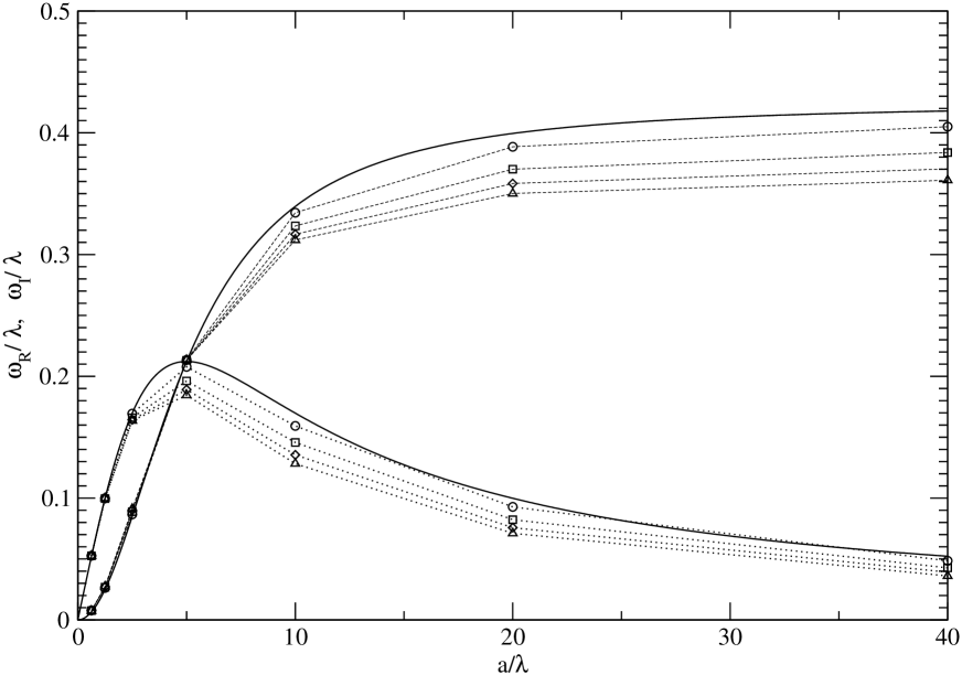
Figure 1: Numerically obtained values of the real and imaginary parts of the eigen frequency, $\omega_{R}$ and $\omega_{I}$ divided by the parameter $\lambda$ as functions of the ratio $a/\lambda$. Solid curves represent analytical results given by equation (97). Dashed and dotted curves represent numerical values of $\omega_{R}$ and $\omega_{I}$, respectively. The various symbol styles indicate different values of $\lambda.$ These are such that smaller values of $\lambda$ lie closer to the analytically determined curves.

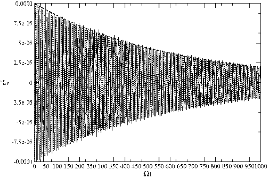
Figure 2: The time dependence of the displacement vector evaluated near the upper boundary of the gas column calculated for models with $\lambda=0.032$. The solid (dotted) curve corresponds to $a=1.26$ ($a=0.02$). Note that both curves practically coincide. The dashed curve represents the exponential dependence of the amplitude of the oscillations on time, being $\propto e^{-\omega_{I}t},$ calculated with the analytically determined value of $\omega_{I}=1.65\cdot 10^{-3}$.

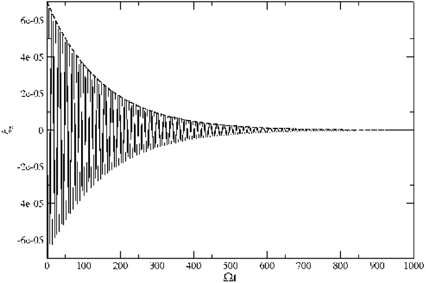
Figure 3: As Figure 2 but with $a=0.16$. This value of $a$ gives the maximal decay rate when $\lambda=0.032$.

The results of our computations are plotted in Figures 1-4. In Figure 1 we show the numerically obtained dependencies of $\omega_{R}/\lambda$ (the dashed curves ) and $\omega_{I}/\lambda$ (the dotted curves) on $a/\lambda$ for the set of parameters described above. Specific symbols are associated with particular values of $\lambda.$ Circles, squares, diamonds and triangles represent the specific values of $\lambda$ we used in increasing order. Solid curves correspond to the analytically determined dependencies given by equation (97). One can see that the agreement between the analytic and numerical results is good for the smallest value of $\lambda=0.032.$ However, the curves deviate more significantly as $\lambda$ is increased. This departure from a dependence of $\omega/\lambda$ only on $a/\lambda$ may be explained as an effect due to the increasing importance of of higher order terms in the power series representation of $\omega/\lambda$ as a function of $\lambda,$ for fixed $a/\lambda,$ that were not taken into account in equations (60) and (61).

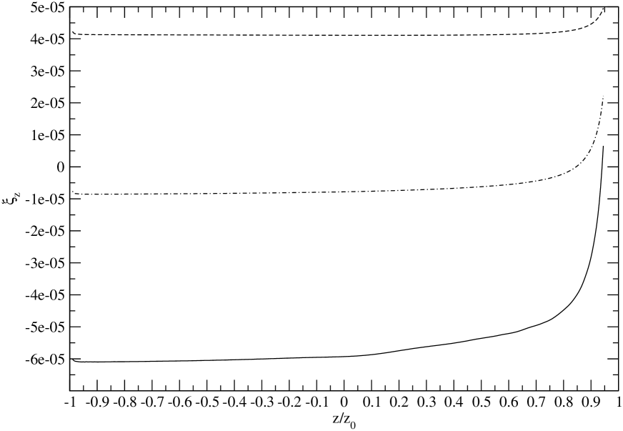
Figure 4: The dependence of the displacement vector on the vertical coordinate $\zeta,$ at a typical time, for $\lambda=0.032$ and different values of $a.$ The solid, dot-dashed and dashed curves correspond to $a=1.26,0.16$ and $0.02$ respectively.

Figure 2 shows the displacement vector evaluated near the boundary $\zeta=\zeta_{0}$ as a function of time for $\lambda=0.032$ with $a=1.26$ (solid curve ) and $a=0.02$ ( dotted curve). Regardless of the fact that these values of $a$ differ, their analytically calculated decay rates are practically the same and such that $\omega_{I}\approx 1.65\cdot 10^{-3}$. As expected the temporal behaviour of the displacement vector is almost indistinguishable for these two cases. The dashed curve indicates the exponential dependence on time, calculated in this case, using the decay rate $\omega_{I}=1.65\cdot 10^{-3}.$ It is evident that agreement between the analytical and numerical results is good.

Figure 3 is similar to Figure 2 but the dependence of the displacement vector on time is shown for $a=0.16.$. Because $a/\lambda=5$ this value of $a$ corresponds to the maximal decay rate when $\lambda=0.032.$ In this case it is given by $\omega_{I}\approx 6.7\cdot 10^{-3}.$ Note again the very good agreement between the theoretical and numerical results.

In Figure 4 we show the dependence of the displacement vector on $\zeta$ calculated at the same time for $a=1.26$ - solid curve, $a=0.16$ - dot-dashed curve and $a=0.02$ -dashed curve. One can see from this Figure that the displacement corresponding to the small value of $a$ is practically independent of $\zeta.$ But for the large value of $a$ it has a prominent increase toward the upper boundary of the column. Also, note that in the latter case the value of displacement vector near the upper boundary is close to zero. Thus, although the time dependence of the displacement vectors corresponding to the cases of large and small $a$ is practically the same, the spacial dependence of these quantities is quite different.

8.2.2 Non linear calculations

Table 1: The initial amplitude of velocity profiles, $C$, the maximal value of the relative pressure difference $(P-P_{0})/P_{0}\equiv\Delta P/P_{0}$ calculated for the first pulsational period and the difference between the final and initial values of the thermal energy per unit area, $\Delta E_{Th}$, for the different models used in the computations. Note that quantities are expressed as multiples of the dimensional units defined in the text.

	$1$	$2$	$3$	$4$	$5$	$6$	$7$	$8$
$C$	$10^{-3}$	$5\cdot 10^{-3}$	$10^{-2}$	$2\cdot 10^{-2}$	$4\cdot 10^{-2}$	$8\cdot 10^{-2}$	$1.6\cdot 10^{-1}$	$3.2\cdot 10^{-1}$
$\Delta P/P_{0}$	$4\cdot 10^{-2}$	$0.2$	$0.4$	$1$	$2.5$	$7$	$20$	$80$
$\Delta E_{Th}$	$9\cdot 10^{-8}$	$1.4\cdot 10^{-6}$	$5.4\cdot 10^{-6}$	$2\cdot 10^{-5}$	$8.6\cdot 10^{-5}$	$4.4\cdot 10^{-4}$	$2\cdot 10^{-3}$	$9\cdot 10^{-3}$

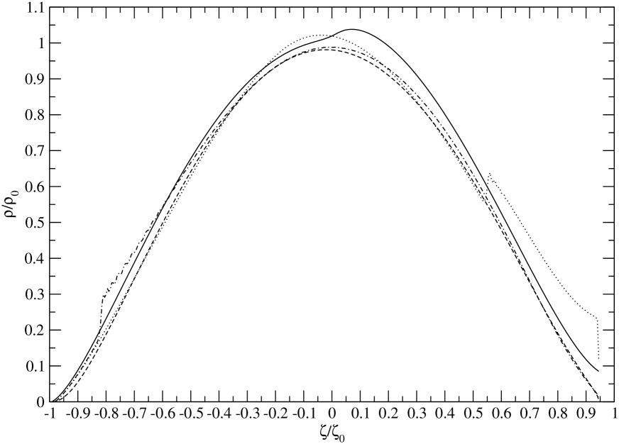
Figure 5: The dependence of density $\rho$ on $\zeta$ at four different times for model $7,$ which is characterised by the relative pressure amplitude $C=0.16$. The solid, dashed, dotted and dash-dotted curves correspond to the times $\tau=2.5,5,7.5$ and $10$, respectively.

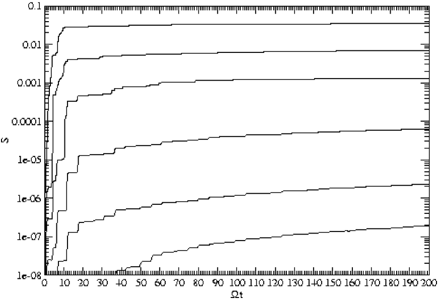
Figure 6: The dependence of the entropy per unit area, $S,$ for the six models $(3-8).$ As the entropy increases while moving from the lowermost to uppermost curve, the models range from $3-8$ with increasing values of the initial amplitude $C$.

In order to determine how our results depend on the initial velocity amplitude, we consider the case for which the upper boundary of the column is a rigid wall, resulting in the condition that $v(\zeta=\zeta_{*})=0$. From our previous discussion it follows that this occurs when the parameter $a$ is sufficiently large. The uniform initial velocity profile used in our previous numerical calculations is not compatible with this boundary condition. Therefore, we use a different initial form for the velocity

$$v=C\cos({\pi\over 2}{\zeta\over\zeta_{*}}).$$ (98)

Since the non-linear effects are expected to operate on a short dynamical time scale of order of a few periods $P=2\pi\Omega^{-1}$ we follow the evolution for relatively small times $\tau_{end}=200.$

When the rigid wall boundary condition is applied and the linear theory is valid, the column dynamics is determined by the linear superposition of strictly periodic oscillations. Departures from this type of motion are determined by non-linear effects. One of the most important for our purposes is the possibility of shock formation near the upper boundary. When such shocks propagate through the column they irreversibly heat up the gas thus causing dissipation of the motion induced in the column.

The strength of non-linear effects is obviously proportional to the induced amplitude $C.$ In the first row of Table 1 we show the eight values of $C$ used in our computations and the corresponding models, enumerated by numbers from one to eight. In all cases we assume that the rigid boundary is situated at the value of $\zeta_{*}$ corresponding to $\lambda=0.032$.

A useful measure of non-linearity of the system is the ratio of the difference between the pressure at the upper boundary and its equilibrium value $\Delta P=P-P_{0},$ to $P_{0}$. For definiteness we estimate the maximal values of this quantity during the first non-linear pulsation and display them in the second row of Table 1. As seen from this Table when $\Delta P/P_{0}<1,$ this quantity has an approximate linear dependence on $C,$ while for larger values this dependence is somewhat steeper. The third row represents the difference between the thermal energy (per unit area) at the end of the computations at $\tau_{end}=200$ and its initial value $E_{th}\approx 0.33$, in units of $P_{c}\zeta_{0}$. As expected this quantity is approximately proportional to the square of $C$.

8.3 Shock development and the formation of a rarefied hot atmosphere

When $\Delta P/P_{0}<1$ the dynamics of the model is well described by the linear theory. In the opposite case, non-linear effects are substantial. The system exhibits a complicated pulsational behaviour and strong shocks are observed. This regime is illustrated in Figure 5 where the results of calculations for model $7,$ with large initial amplitude $C=0.16,$ are presented. We show the density profiles at four different times $\tau=2.5$ ( solid curve ), $\tau=5$ (dashed curve ), $\tau=7.5$ ( dotted curve ) and $\tau=10$ ( dot dashed curve ). The density distribution at $\tau=2.5$ is quite similar to the equilibrium density distribution. When $\tau=5$ and $\tau=7.5$ shocks are observed propagating from the upper boundary in the direction of negative $\zeta$. These shocks heat the gas up, thus dissipating kinetic energy. Also note the density drop at the upper boundary when $\tau=5$ and $\tau=10$. We have checked that this density drop has a persistent character and the density at the boundary at $\tau=\tau_{end}$ is significantly smaller than the initial density while the pressure does not exhibit such a significant change.

Thus, the presence of shocks in the system leads to formation of a hot rarefied region near the rigid boundary. It is not clear however, how this effect would operate in twisted discs. In the latter case the boundary is defined by the condition that the optical thickness is one. The position of this boundary may move when any density redistribution becomes significant. In our case with fixed upper boundary location, the presence of this hot low density region leads to the suppression of shock formation after a time corresponding to a few orbital periods, an effect that may not occur if the upper boundary moved in such a way as to maintain the relative pressure variations.

The effect in our case is illustrated in Figure 6 where we show the dependence of entropy per unit area, $S=\int d\zeta\rho\log(p/\rho^{\gamma})$ as a function of time for the models with indices larger than $2$, in the natural units $\rho_{c}\zeta_{0}.$ Curves attaining larger values correspond to larger amplitudes. One can see from this Figure that when the initial amplitude is sufficiently large, i.e. $C\geq 0.04$ and accordingly $\Delta P/P_{0}\geq 2.5,$ half of the entropy change is roughly determined for $\tau<10-15.$ (i.e. approximately during the first two orbital periods). Then shock production becomes less efficient due to the mechanism discussed above.

8.4 Estimate of dissipation time scale

As mentioned above, it is not clear to what extent the dynamics of the column in the strongly non linear regime is similar to the non-linear dynamics of twisted discs. One can assume, e.g. that in twisted discs, the boundary where external radiation pressure applies follows a certain density level. In this situation it seems reasonable to assume that the shock formation might persist at a rate similar to what is observed at initial times $\tau<10$. In this case the disc perturbations could be damped on a time scale $t_{nl}$ which can be roughly estimated from the results presented in Figure 1.

For model $7,$ assuming the thermal energy production is of the order of $\Delta E_{th}=0.002,$ we can estimate the non linear decay time as $t_{nl}\sim 10(E_{th}/\Delta E_{th})\Omega^{-1}\sim 1.5\cdot 10^{3}\Omega^{-1}$ where we recall that $E_{th}\approx 0.3$ in our units. Thus, under these assumptions the perturbations may decay in approximately $200$ orbital periods. This rate is characteristically the internal energy content within one surface scale height per orbital period and becomes noticeable when the relative pressure variation $\Delta P/P_{0}$ near the upper boundary exceeds $\sim 2.5.$

Let us stress, however, that although indicative, because of an obvious sensitive dependence on the density structure near the boundary, such an estimate cannot be rigorously justified within our model. Clearly more comprehensive future investigations are needed.

9 Discussion and Conclusions

In this paper we have presented a self-consistent calculation of the response of a twisted disc to the action of a radiation pressure force acting in upper layers of the disc. This is assumed to be due to the interception and subsequent reradiation of radiation from a central source. The radiation pressure force is assumed to be applied at a single density level $\rho_{*}$ corresponding to optical thickness unity. The degree of twist and warping is assumed to be small enough that linear theory can be used to calculate the response.

The analysis of Pringle 1996 modelled the disc as a set of concentric rigid rings in a state of Keplerian rotation. These were assumed to communicate with each other through the exchange angular momentum because of the action of viscous forces. Up to now there has been no consideration of effects arising from the response of the disc vertical structure to the externally applied pressure.

In this paper we have considered the warping and twisting of an accretion disc taking account the response of the disc vertical structure to an external radiation field assuming that the effect of self-shielding of radiation by the global twisted disc is not significant. We developed a description of the evolution of the disc in terms of a pair of equations governing the one dimensional evolution of the inclination as a function of radius and time (see section 6 and equations (41), (67) and (68)). This description extends earlier ones, so that the influence of radiation pressure on discs for which warps occur in the low viscosity bending wave regime, as well as the higher viscosity diffusive regime, may be considered.

We found several qualitatively different dynamical regimes that may be realised in astrophysical discs. These are related to whether the character of the response of the disc vertical structure causes significant departures from what would be obtained for a rigid body.

9.1 Conditions for a quasi-rigid response

We found that to avoid such departures, the momentum flux due to radiation from the central source $F_{0},$ should be smaller than a critical value, $F_{*},$ given by $F_{*}=(\lambda/\delta)P_{c},$ where $\delta=\zeta_{0}/r$ is the disc aspect ratio, $P_{c}$ is the disc mid plane pressure and it has been assumed that the the ratio $(\lambda/\delta)$ is small (see sections 6.5 and 7.1.2). Then, when $F_{0}>F_{crit}\approx 0.1(\delta/\alpha)P_{c},$ warping instability of the disc becomes a possibility ( eg. Pringle, 1996).

Thus for radiation driven warping of a disc that behaves like an ensemble of rigid rings, we find two requirements, namely that $F_{*}>F_{crit},$ together with $F_{0}<F_{*}.$ These conditions together imply that the ration of the surface to mid plane density should be sufficiently large and such that $\lambda>\lambda_{crit}\approx 0.1\delta^{2}/\alpha.$

9.2 Large external radiation momentum flux

In the opposite limit of large $F_{0}>max(F_{*},F_{crit}),$ consideration of the disc structure in the vertical direction is essential as the vertical displacement ceases to be uniform. The perturbed gas motion in the disc is mainly determined by the vertical component of velocity and the perturbed quantities tend to oscillate at a characteristic frequency $\omega=(\rho_{c}\zeta_{0}/2\Sigma)\lambda\Omega$, with $\Omega$ being the local Keplerian angular velocity. In this situation, vertical motion tends to be suppressed by the external pressure field on the irradiated side of the disc while warping motions persist in the bulk of the disc and on the shielded side of the disc (see sections 6.5 and 7.2).

The disc surface intercepting the radiation tends to align parallel to the radiation rays, thus decreasing the amount of intercepted radiation, while the inclination angles associated with the disc mid plane and the opposite free boundary of the disc oscillate, being approximately equal to each other. In this limit the upper surface of optical thickness one plays the role of an impenetrable wall. Thus the development of instability of the inclination angle due to radiation pressure effects (e.g. Pringle 1996) would be inhibited in this limit.

In principle, the presence of warping motions in this regime would be associated with variability on a large characteristic time scale $T_{ch}\sim\lambda^{-1}T_{K}$, where $T_{K}$ and $\lambda$ are some ’typical’ values of the orbital period and the density ratio.

9.3 Limits on the WKB growth rate

Following Pringle 1996 we have considered possible instabilities using a WKB approach. As this neglects potentially important global effects and boundary conditions results are not definitive, nonetheless they should give a good indication of when instability could be possible.

We find that when $F_{0}<F_{*}$ the growth rate increases with $F_{0}$ while in the formal limit $F_{0}\rightarrow\infty$ it approaches zero. Thus in the linear theory there is an upper limit for the growth rate of the instability of the inclination angle which is always $\leq(\rho_{c}\zeta_{0}/\Sigma)\lambda\Omega$ in the absence of viscosity (see section 7.3). When present, viscosity acts to damp any instability at a rate $0.1\delta^{2}\Omega/\alpha,$ leading again to the condition $\lambda>\lambda_{crit}\approx 0.1\delta^{2}/\alpha$ for radiation warping instability to be feasible.

9.4 Conditions for non-linearity

Our results described above rely upon the applicability of linear perturbation theory. As discussed in section 7.5, the breakdown of linear theory is expected when the Lagrangian change of pressure induced in the surface layers becomes of the order of the unperturbed pressure even though the change of inclination angle could be very small. The corresponding constraints on the inclination angle are especially strong for disc models with a significant drop of temperature toward the boundaries of the disc.

9.5 Non linear calculations for the one dimensional slab analogue

A direct numerical approach to the issues discussed above is not yet feasible due to three-dimensional nature of the problem and the many physical processes involved. However, when vertical motions dominate, the problem becomes analogous to the one dimensional problem of vertical motions induced in a stratified gas column orbiting around a central source with Keplerian angular velocity.

As discussed in Section 8 the one dimensional slab gives the same fundamental period of oscillation as obtained from the full disc theory when an appropriate boundary condition on the upper surface of the column is specified. The dependence of the eigenfrequency on theoretical parameters as well as the effective presence, in the limit of small $\lambda,$ of an impenetrable wall at the upper surface of the column have been checked numerically. Where they can be compared, agreement between our analytical and numerical results is very good.

We also used the one dimensional model in order to investigate possible consequences of non-linear behaviour in the system. To do this we studied the motion of the slab ensuing from the imposition of a vertical velocity profile with varying amplitude. We found that when the ratio of the Lagrangian pressure perturbation to the local value of the pressure at the upper boundary of the disc, $\Delta P/P_{*}$, becomes larger than $1-10,$ strong shocks propagating downward into the column are observed (see section 8.3). In principle, these shocks may lead to non-linear dissipation of energy stored in the vertical motion and in section 8.4 we made a very crude estimate of a possible time scale of $200$ orbits for $\Delta P/P_{*}\sim 10$. However, this result must be checked in framework of a more sophisticated numerical approach which takes into account physical processes neglected in this study, most notably the effects of radiation transfer in the upper layers of the column.

9.6 Issues for future consideration

In a fully self-consistent study the dynamical effects of radiation pressure must be studied together with effects determined by the radiation heating of the disc atmosphere. This can be done in the most convenient way within the framework of the one dimensional model discussed above.

In a realistic disc model, where effects due to the flaring of the disc lead to the interception and scattering of radiation in the disc photosphere, when axisymmetric and unperturbed, radiation heating can significantly influence on or even determine the value of the density ratio $\lambda.$

This parameter, being the ratio of the density at the absorbing surface to the mid plane density defines the boundary between different dynamical regimes for a twisted disc. In this connection it is interesting to note that in certain vertical models of X-ray heated accretion discs, the ratio $\lambda$ can be quite small, being of order of $10^{-4}-10^{-5}$, e.g. Jimenez-Garate et al 2002. In such models the new dynamical effects discussed in this Paper would certainly play an important role.

Appendix A Expression for radiation pressure acting on the disc surface

Expressions for the radiation pressure acting on a surface element of a twisted disc (or, alternatively an expression for the corresponding torque acting on a disc annulus of radius $r$) have been derived by a number of authors, e.g. Petterson 1977b, Pringle 1996, Ogilvie $\&$ Dubus 2001, under different approximations. However, these authors assume that the disc consists of rigid rings of different radii having differing inclinations and orientations with respect to a fixed Cartesian coordinate system, when deriving the corresponding expressions. This assumption is essentially equivalent to the statement that all vertical motions can be accounted for by a rigid tilt and it precludes internal vertical motions that vary with the vertical coordinate.

As discussed in the main text, this is not strictly valid, as in general such motions occur. Accordingly, the density surfaces corresponding to an optical thicknesses of order of unity where the radiation pressure force is applied are not everywhere parallel to the surface locally corresponding to the disc mid-plane and the expression for the radiation pressure acting on the disc must be, accordingly modified.

In general, an expression describing the surfaces of constant optical thickness can be easily obtained from the transformation law from the Cartesian coordinate system to the twisted coordinate system written for a gas element situated near the surface of the disc

$$x=r\cos\phi\pm\beta\zeta_{0}\sin\gamma,\quad y=r\sin\phi\mp\beta\zeta_{0}\cos\gamma,$$ (99)

and

$$z=\pm\zeta_{0}+\xi^{\zeta}(\zeta\rightarrow\zeta_{0})+r\beta\sin(\phi-\gamma),$$ (100)

where the upper (lower) sign corresponds to the upper (lower) disc surface. Let us recall that we assume that the inclination angle $\beta$ is small and derive all equations in the linear approximation for the angle $\beta$ and the Lagrangian displacement vector $\bar{\xi}$.

The unit vector perpendicular to the disc surface is given by the standard expression

$$\bar{n}={\partial\bar{R}\over\partial r}\times{\partial\bar{R}\over\partial\phi}{\rm{\huge{/}}}\left|{\partial\bar{R}\over\partial r}\times{\partial\bar{R}\over\partial\phi}\right|,$$ (101)

where $\bar{R}$ is the radius vector with components $(x,y,z)$.

We make the standard assumption that the radiation propagates radially before being intercepted by the disc and neglect the effect of self-shielding. In this case an amount of radiation intercepted by the disc and subsequently reradiated away is proportional to cosine of angle between the radius vector and the normal to the disc, $\cos\Xi\equiv\bar{{n}}\cdot\bar{{R}}/|\bar{{R}}|$. For the upper branch of the surface a simple calculation gives

$$\cos\Xi=-r{\partial\over\partial r}{(\zeta_{0}+\xi^{\zeta})\over r}-r{\cal}{\cal W},$$ (102)

where we recall that ${\cal W}=\beta^{{}^{\prime}}\sin\psi-\beta\gamma^{{}^{\prime}}\cos\psi=\Psi_{1}\sin\phi-\Psi_{2}\cos\phi$. As we discuss in the main text, in this paper, for simplicity, we neglect the effect of disc flaring and accordingly set ${\partial\over\partial r}({\zeta_{0}\over r})=0$ in equation (102).

The upper (lower ) branch of the disc surface is able to intercept the radiation of a central source only when $\cos\Xi<0$ ( $\cos\Xi>0$). Therefore the radiation pressure, $F$, applied to the disc surface has the form

$$F_{\pm}=\mp\Theta(\mp\cos(\Xi)){2\over 3}F_{0}\cos(\Xi),$$ (103)

where $\Theta(x)$ is the step function, the signs $(+)$ and $(-)$ stand for the upper and lower branches of the disc surface, respectively,

$$F_{0}={L\over 4\pi cr^{2}}$$ (104)

is the momentum flux per unit of surface carried by the radiation emitted by the central source, and $L$ is the luminosity of the source. The factor $(2/3)$ accounts for (assumed ) isotropic character of the disc reradiation.

In order to have the same symmetries as the surface pressure term (103) the $\zeta$-component of the displacement vector, $\xi^{\zeta}$, and, accordingly, the $\zeta$-component of velocity perturbation, $v^{\zeta}$, must satisfy

$$\xi^{\zeta}(\zeta,\phi)=-\xi^{\zeta}(-\zeta,\phi+\pi),\quad v^{\zeta}(\zeta,\phi)=-v^{\zeta}(-\zeta,\phi+\pi).$$ (105)

On the other hand, for a given value of $\phi$, $v^{\zeta}$ may be separated on even and odd components: $v^{\zeta}=v_{e}^{\zeta}+v_{o}^{\zeta}$ and both components should be taken into account in order to satisfy the appropriate boundary conditions at $\zeta\rightarrow\pm\zeta_{0}$. However, the latter requirement poses a problem with the symmetry law (105). Indeed, while the even part of $v^{\zeta}$, $v_{e}^{\zeta}$, agrees with (105) the odd one is not and the standard separation of the velocity perturbations into even and odd parts although being respected by the perturbed equations of motion, is not, strictly speaking, compatible with the symmetries provided by the boundary conditions. This problem can be circumvented with the help of the assumption that the normal decomposition into even and odd parts in $\zeta$ of the perturbed vertical velocity is replaced by

$$v^{\zeta}=v^{\zeta}_{e}-sign(\sin(\phi-\phi_{1}))v^{\zeta}_{o},$$ (106)

where $v^{\zeta}_{e}$ and $v^{\zeta}_{o}$ have even (odd ) properties with respect to the reflection $\zeta\rightarrow-\zeta$. Since the surface radiation pressure vanishes when $\cos\Xi=0$ or equivalently $\sin(\phi-\phi_{1})=0$ and, accordingly, we have $v^{\zeta}_{o}=0$ at the corresponding values of $\phi=\phi_{1}$ and $\phi=\phi_{1}+\pi$ the velocity anzatz (106) is self-consistent. Also, it agrees with the symmetries determined by equation (103) and it has local simmetries respected by the equations of motion.

Above and in the main text we always consider the angle $\phi$ to be in a segment $[\phi_{1}..\phi_{1}+\pi]$ defined by the condition $\sin(\phi-\phi_{1})>0.$ With help of this convention we can treat our dynamical variables as having the standard even and odd symmetries with respect to reflection $\zeta\rightarrow-\zeta.$ Continuation of these variables into the segment defined by condition $\sin(\phi-\phi_{1})<0$ can be made with the help of the expression (106). In the case when $\sin(\phi-\phi_{1})>0$ it follows from equations (102) and (103) that we have

$$F(\rho=\rho_{*},\zeta\rightarrow\zeta_{0})\equiv F_{+}={2\over 3}F_{0}r{d\over dr}\left({\xi^{\zeta}\left(\rho_{*}\right)\over r}+{\cal W}\right),$$ (107)

and

$$F(\rho=\rho_{*},\zeta\rightarrow-\zeta_{0})\equiv F_{-}=0,$$ (108)

where we recall that the density $\rho_{*}$ corresponds to the surface of an unperturbed disc with optical thickness $\tau\approx 1.$ Taking into account that we can write $F_{+}=F_{+}^{1}\cos\phi+F_{+}^{2}\sin\phi$ and $\xi^{\zeta}=\xi_{1}^{\zeta}\cos\phi+\xi_{2}^{\zeta}\sin\phi$, we can represent equation (107) in a convenient complex form

$${\bf F}_{+}={2\over 3}F_{0}r{d\over dr}\left({\bf\xi}^{\zeta}/r+i{\bf W}\right),$$ (109)

where ${\bf F}_{+}=F_{+}^{1}+iF_{+}^{2}$, ${{\xi}}_{\zeta}=\xi_{1}^{\zeta}+i\xi_{2}^{\zeta}$ and ${\bf W}=\beta e^{i\gamma}=\Psi_{1}+i\Psi_{2}$. Obviously, we also have ${\bf F}_{-}=0$.

Appendix B Solution of equation (45) for the case of arbitrary $\gamma$

When the parameter $\gamma>1$ is not specified, the homogeneous equation (45) can be reduced to a simpler form with help of equations (10) and (11). We get

$$(1-x^{2}){d^{2}\over dx^{2}}{\bf v}-{2\gamma x\over\gamma-1}{d\over dx}{\bf v}+{4\over\gamma-1}\tilde{\omega}{\bf v}=0,$$ (110)

where $x=\xi/\xi_{0}$. A general solution of (110) has the form

$${\bf v}=(1-x^{2})^{-{1\over\gamma-1}}\left(C_{1}F({1\over 2}-\alpha,{1\over 2}-\beta,{1\over 2},x^{2})+C_{2}xF(1-\alpha,1-\beta,{3\over 2},x^{2})\right),$$ (111)

where $F(\alpha,\beta,\delta,x)$ is the hyper-geometric function and

$$\alpha,\beta={\gamma+1\over 4(\gamma-1)}(1\pm\sqrt{1+{64(\gamma-1)\over(\gamma+1)^{2}}\tilde{\omega}}).$$ (112)

. When $\tilde{\omega}\ll 1$ we have

$$\alpha\approx{\gamma+1\over 2(\gamma-1)}+{8\over\gamma+1}\tilde{\omega},\quad\beta\approx-{8\over\gamma+1}\tilde{\omega}.$$ (113)

Appendix C The gauge transformations

As we pointed out in the main text different twisted coordinate systems can describe the same physical situation provided that they are connected by a certain family of transformations (gauge transformations) which maintain fixed distributions of physical quantities characterising the system (density and velocity fields in the case of a baratropic gas) in a non rotating (say, cylindrical) coordinate system with origin located at the central source. These transformation laws can be found by considering transformations from the cylindrical to the twisted coordinates. We derive them here assuming, for simplicity, that the equation of state is baratropic and the gas is inviscid. The latter assumption allows us to neglect the presence of the radial component of velocity in an unperturbed background state.

We begin by considering the transformation of density. Let the density $\rho$ be represented in the cylindrical and twisted coordinate systems as

$$\rho=\rho_{0}(r_{c},z_{c})+\rho_{1}^{c}(r_{c},z_{c})=\rho_{0}(r,\zeta)+\rho_{1}(r,\zeta),$$ (114)

where the background part $\rho_{0}$ has the same functional dependence on the cylindrical and twisted coordinates. The cylindrical and twisted coordinates are related to each other by transformations (16)-(18). Substituting these transformations in equation (114) we obtain

$$\rho_{1}^{c}(r,\zeta)=\rho_{1}(r,\zeta)+D\beta\sin(\phi-\gamma),$$ (115)

where

$$D=\left(\zeta{\partial\over\partial r}-r{\partial\over\partial\zeta}\right)\rho_{0}.$$ (116)

By construction the quantity $\rho_{1}^{c}$ is not changed after a gauge transformation. Therefore, it may be classified as a ’gauge independent’ quantity. The result (115) can be represented in a compact form with help of the complex notation introduced in equation (19)

$${\bf\rho}_{1}^{c}={\bf\rho}_{1}+iD{\bf W}.$$ (117)

In an absolutely analogous way we can find the law of transformation of velocity perturbations. We have

$${\bf v}^{\phi_{c}}={\bf v}^{\phi}+\zeta(i(r\Omega)^{{}^{\prime}}{\bf W}-\dot{\bf W}),$$ (118)

$${\bf v}^{z_{c}}={\bf v}^{\zeta}+ir\dot{\bf W}+r\Omega{\bf W},$$ (119)

and

$${\bf v}^{r_{c}}={\bf v}^{r}-i\zeta\dot{\bf W}-\zeta\Omega{\bf W}.$$ (120)

Here the quantities ${\bf v}^{\phi_{c}}$, ${\bf v}^{z_{c}}$ and ${\bf v}^{r_{c}}$ represent the velocity perturbations in the cylindrical coordinate system. They are gauge independent by construction. The quantities ${\bf v}^{\phi}$, ${\bf v}^{\zeta}$ and ${\bf v}^{r}$ represent the time derivative of the corresponding coordinates of a comoving gas element. As we discussed above these quantities do not coincide with the projections of velocity onto the orthonormal basis used in the formalism exploiting the twisted coordinate system. The relations between these projections and the time derivatives of the coordinates can be easily found from the results provided in the Appendix of Petterson 1978, his equations (A3). They can be written in the form

$$\hat{\bf v}^{\phi}={\bf v}^{\phi}-\zeta\dot{\bf W},\quad\hat{\bf v}^{\zeta}={\bf v}^{\zeta}+ir\dot{\bf W},\quad\hat{\bf v}^{r}={\bf v}^{r}-i\zeta\dot{\bf W},$$ (121)

where it is implied that the background parts of the $(\zeta)$ and $(r)$-components of velocity can be neglected. Substituting equations (121) in equations (118)-(120) we find

$${\bf v}^{\phi_{c}}=\hat{\bf v}^{\phi}+i\zeta(r\Omega)^{{}^{\prime}}{\bf W},$$ (122)

$${\bf v}^{z_{c}}=\hat{\bf v}^{\zeta}+r\Omega{\bf W},$$ (123)

and

$${\bf v}^{r_{c}}=\hat{\bf v}^{r}-\zeta\Omega{\bf W}.$$ (124)

Now let us suppose that there are two twisted coordinate systems with two different ${\bf W}_{1}$ and ${\bf W}_{2}$ describing the same physical system. That means that the quantities characterising the density perturbation and perturbations of the velocity field in the fixed cylindrical system must be the same when expressed in terms of Euler angles and corresponding perturbations belonging to the different twisted coordinate systems. From this requirement and equations (117) and (122)-(124) it follows that the differences in the corresponding to these systems perturbations of density and velocity components must be proportional to the difference between ${\bf W}_{1}$ and ${\bf W}_{2}$, $\delta{\bf W}={\bf W}_{1}-{\bf W}_{2}$,

$$\delta{\bf\rho}_{1}=-iD\delta{\bf W},$$ (125)

$$\delta\hat{\bf v}^{\phi}=-i\zeta(r\Omega)^{{}^{\prime}}\delta{\bf W},$$ (126)

$$\delta\hat{\bf v}^{\zeta}=-r\Omega\delta{\bf W},$$ (127)

and

$$\delta\hat{\bf v}^{r}=\zeta\Omega\delta{\bf W}.$$ (128)

Equations (125)-(128) define the gauge transformations between two twisted coordinate system for an inviscid disc. Viewed in these terms, the generalisation to the case of a viscid disc is straightforward provided that the background part of the $(r)$-component of velocity is taken into account.

One can also check that equations (125)-(128) provide an exact solution of the equations of motion and the continuity equation for an inviscid disc being written in a twisted coordinate system, for an arbitrary dependence of ${\bf W}$ on $t$ and $r$. This solution describes the so-called trivial modes corresponding to an unperturbed disc. In this case the density and velocity fields in the cylindrical coordinate system remain equal to their unperturbed values while the dynamics in the twisted coordinates is such that perturbations of density and velocity defined with respect to the twisted coordinates are exactly compensated by those associated with time dependent Euler angles.

It is important to stress that our dynamical equations (23) and (25) as well as the continuity equation (29) are not invariant under the transformations generated by (125)-(128) even when the term determined by viscosity are discarded. This is due to the fact that certain terms are neglected in these equations. These terms provide only next order corrections in our expansion series in small parameters when the gauge (57) is fixed. On the other hand the combination ${\bf\xi}^{\zeta}/r+i{\bf W}$ entering in the expression (109) determine an invariant quantity - the angle between the normal to the disc surface and the radial direction. This combination must be the same in all twisted coordinate systems connected by transformations (125)-(128). Using equations (37) and (121) it is easy to see that this combination is proportional to

$$\hat{\bf v}^{\zeta}+r\Omega{\bf W}.$$ (129)

From equation (127) it follows that the expression (129) is, indeed, a gauge invariant quantity.

References

- (1) Clarkson, W. I., Charles, P. A., Coe, M. J., Laycock, S., 2003, MNRAS, 343, 1213
- (2) Demianski, M., Ivanov, P. B., 1997, AA, 324, 829
- (3) Foulkes, S. B., Haswell, C. A., Murray, J. R., 2006, MNRAS, 285, 1399
- (4) Hatchett, S. P., Begelman, M. C., Sarazin, C. L., 1981, ApJ, 247, 677
- (5) Ivanov, P. B., Illarionov, A. F., 1997, MNRAS, 285, 394
- (6) Iping, R. C., Petterson, J. A., 1990, A&A, 239, 221
- (7) Jimenez-Garate, M. A., Raymond, J. C., Liedahl, D. A., 2002, ApJ, 581, 1297
- (8) Katz, J. I., 1973, Nature, 246, 87
- (9) Landau, L. D., Lifshitz, E. M., 1975, ’The classical theory of fields’, Oxford: Pergamon Press, 4th rev. Eng. ed.
- (10) Maloney, P. R., Begelman, M. C., Nowak, M. A., 1998, ApJ, 504, 77
- (11) Nelson, R. P., Papaloizou, J. C. B., 1999, MNRAS, 309, 929
- (12) Nelson, R. P., Papaloizou, J. C. B., 2000, MNRAS, 315, 570
- (13) Ogilvie, G. I., Dubus, G., 2001, MNRAS, 320, 485
- (14) Papaloizou, J. C. B., Lin, D. N. C., 1995, ApJ, 438, 841
- (15) Papaloizou, J. C. B., Pringle, J. E., 1983, MNRAS, 202, 1181
- (16) Petterson, J. A., 1975, ApJ, 201, L61
- (17) Petterson, J. A., 1977, ApJ, 214, 550 (a)
- (18) Petterson, J. A., 1977, ApJ, 216, 827 (b)
- (19) Petterson, J. A., 1978, ApJ, 226, 253
- (20) Pfeiffer, H. P., Lai, D., 2004, ApJ, 604, 766
- (21) Pringle, J. E., 1996, MNRAS, 281, 357
- (22) Quillen, A. C., 2001, ApJ, 563, 313
- (23) Richtmyer, R. D., Morton, K. W., 1967, ’Difference methods for initial-value problems’, Interscience publishers, John Wiley Sons, New York London Sydney, 2d ed.
- (24) Shakura, N. I., Sunyaev, R. A., 1973, AA, 24, 337