Memory Effects in the Standard Model for Glasses.

Abstract

The standard model of glasses is an ensemble of two-level systems interacting with a thermal bath. The general origin of memory effects in this model is a quasi-stationary but non-equilibrium state of a single two-level system, which is realized due to a finite-rate cooling and very slow thermally activated relaxation. We show that single particle memory effects, such as negativity of the specific heat under reheating, vanish for a sufficiently disordered ensemble. In contrast, a disordered ensemble displays a collective memory effect [similar to that described by Kovacs for glassy polymers], where non-equilibrium features of the ensemble are monitored via a macroscopic observable. An experimental realization of the effect can be used to further assess the consistency of the model.

Introduction. Low temperature properties of glassy and amorphous materials have been an active field of research for more than 30 years anderson ; see review for a review. Experiments have shown that many characteristics of amorphous materials, e.g., the temperature dependence of the specific heat, are universal but different frome those of crystals. This evidence has captivated much interest in the attempt of producing a coherent theoretical picture anderson ; review . The two-level system (TLS) model was one of the first models to fit the experiments. It soon showed to be very successful in describing the low-temperature properties of glasses, e.g., the linear temperature dependence of the specific heat, and gained for itself the definition of “Standard Model” for glasses review . With time this model was improved to account for more features of amorphous solids review and found applications in describing low-temperature features of proteins frau . A drawback of the model is that there is an excessive freedom in choosing the distribution of the ensemble parameters.

Memory effects arise in the model when due to cooling down to low temperatures the thermal activation is impeded huang . Thus the relaxation time increases to an extent that for realistic observation times each TLS is frozen in a non-equilibrium, quasi-stationary state, which—in contrast to its equilibrium analog—depends on the history of the relaxation huang . Most visible effects of this non-equilibrium appear during the subsequent reheating, when due to thermal reactivation the single system specific heat becomes negative amjp . We shall show however that this single particle memory effects do not survive the averaging over a sufficiently disordered ensemble. In contrast, we propose to implement a memory effect, where due to the disorder in the ensemble, locally non-equilibrium features of the system are monitored via a macroscopic (disorder averaged) observable. This effect resembles the one implemented by Kovacs for glassy polymers kovacs . Once the shape of the effect is sensitive to dynamic (relaxation) and static (disorder) features of the model, its experimental verification would constitute a way to further assess the consistency of the model. Analogs of the Kovacs effect were recently studied for several models of glasses kov .

Figure 1: Upper level occupation $n$ vs. dimensionless temperature $T/V$ for a single TLS with $\varepsilon/V=0.2$. Thick curve: $n_{eq}$. The pairs of normal curves refer to cooling (upper curves) and reheating (lower curves) with dimensionless rate (from top to bottom) $\sigma=0.01,\,0.001,\,0.0001$.

The standard model of glasses amounts to independent particles, each one moving in an asymmetric double-well potential with $\varepsilon$ and $V$ being the energy difference between the wells and the barrier height, respectively anderson ; review . Each particle couples to a thermal bath. The positive variables $\varepsilon$ and $V$ change from one particle to another, so that to become observables the single-particle characteristics, such as energy or specific heat, should be averaged over the joint distribution $P(\varepsilon,V)$ of $\varepsilon$ and $V$. The form of $P(\varepsilon,V)$ is well accounted for in literature review :

$$P(\varepsilon,V)=p_{\varepsilon}(\varepsilon;\varepsilon_{\rm max},\varepsilon_{\rm min})\,\,p_{V}(V;V_{\rm min},V_{\rm max}),$$ (1)

where $p_{\varepsilon}$ and $p_{V}$ are flat distributions with $\varepsilon_{min}<\varepsilon<\varepsilon_{\rm max}$ and $V_{min}<V<V_{\rm max}$.

There are two regimes in the motion of the single system. i) The thermally activated regime is realized when the bath-particle coupling is sufficiently large. At each moment of time the particle is then effectively in one of the wells, making sudden jumps between them. The classical two-state approach is thus a good description of this regime. ii) For low temperatures and weak particle-bath couplings only the lowest two energy levels of the quantum double well Hamiltonian are relevant and the problem reduces to a quantum TLS coupled to a bath review . Here we study only the classical regime.

Figure 2: Specific heat $C$ for a single TLS vs. dimensionless temperature $T/V$ and $\varepsilon/V=0.2$. Thick curve: equilibrium $C$. Normal curves: $C$ during protocol (4) with (from left to right) $\sigma=0.0001,0.001,0.01$. Dashed curves: the continuation of each previous cooling protocol by heating with the same $\sigma$ (with opposite sign), starting at $T/V=10^{-4}$, i.e. when $n$ has already relaxed to its zero temperature value.

Let $n$ and $1-n$ be the probabilities for the particle to be in the higher and lower well, respectively. Within the thermally activated dynamics one has:

$$\dot{n}=\gamma_{0}e^{-\beta(V+\varepsilon)}(1-n)-\gamma_{0}e^{-\beta V}\,n,$$ (2)

where $e^{-\beta(V+\varepsilon)}$ and $e^{-\beta V}$ are the rates of the inter-well motion, $T=1/\beta$ is the bath temperature, and where $\gamma_{0}$ is the attempt frequency. Eq. (2) is solved as

$$n_{t}=e^{-\frac{t}{\tau}}(n_{0}-n_{eq})+n_{eq},\quad\tau=e^{\beta V}/[\gamma_{0}(1+e^{-\beta\varepsilon})],$$ (3)

where $\tau$ is the relaxation time and $n_{eq}(\beta)=1/({\rm e}^{\beta\varepsilon}+1)$ the equilibrium value of $n$ reached for $t\gg\tau$. At low temperatures the relaxation time $\tau$ becomes very large, since there is no enough energy for thermal activation. In this regime a freezing temperature $T^{*}$ can be defined (see review ) below which $n$ is essentially frozen-in at $T=T^{*}$.

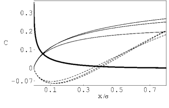
Figure 3: Specific heat $C$ versus $x/\sigma={\sigma}^{-1}e^{-V/T}$ for a single TLS with $\varepsilon/V=0.2$. Thick curve: equilibrium $C$. Normal (dashed) curves: $C$ got via cooling (reheating) protocol (4). From top to bottom: $\sigma=15\times 10^{-6},10^{-4},0.001$.

Cooling. Assume that the bath temperature is cooled according to the following non-linear protocol:

$$\beta_{t}\equiv 1/T_{t}=\beta_{0}+\omega t$$ (4)

where $\omega>0$ is the dimensional cooling rate. This protocol is reasonable for low $T$, since it satisfies the third law, not allowing cooling to $T=0$ in a finite time. Expectedly, for a small rate $\omega$ and a high temperature $T_{t}$, $n$ sticks to its equilibrium value $n_{eq}(\beta_{t})$ while for lower $T_{t}$ there will not be sufficient time to reach this value, since $\tau$ increases; see Fig. 1. We rewrite (2) as:

$$\sigma\frac{{\rm d}n}{{\rm d}x}=(x^{\mu}+1)n(x)-x^{\mu},~{}~{}~{}\sigma\equiv\frac{\omega V}{\gamma_{0}},~{}~{}~{}\mu\equiv\frac{\varepsilon}{V},$$ (5)

where the variable $x_{t}\equiv\exp(-\beta_{t}V)$ is introduced and $\sigma$ is the dimensionless cooling rate. The solution of (5) is:

$$n(x) = n(x_{0})\exp{[\frac{x-x_{0}}{\sigma}+\frac{x^{\mu+1}-x_{0}^{\mu+1}}{\sigma(\mu+1)}]}$$ (6)

$$+ \int_{x}^{x_{0}}\frac{{\rm d}z}{\sigma}\,z^{\mu}\,\exp{[\frac{x-z}{\sigma}+\frac{x^{\mu+1}-z^{\mu+1}}{\sigma(\mu+1)}]},$$

where $x_{0}\equiv\exp(-V/T_{0})$. Note from (6) that the memory about the initial condition $x_{0}$ is eliminated for $x_{0}\gg\sigma$. If this is satisfied and if $\sigma$ is small, the integral in (6) is approximated as [$a(z)\equiv z^{\mu}$, $b(z)\equiv z+z^{\mu+1}/(\mu+1)$]:

$$\int_{x}^{x_{0}}{\rm d}z\,a(z)\,e^{-\frac{b(z)}{\sigma}}\simeq\frac{\sigma a(x)}{b^{\prime}(x)}e^{-b(x)/\sigma}.$$ (7)

Eqs. (6, 7) leads to the equilibrium value of $n$: $n(t)=x^{\mu}/(1+x^{\mu})=n_{eq}(\beta(t))$ This, however, holds under neglection of terms $a^{\prime}(x)(z-x)$ and $b^{\prime\prime}(x)(z-x)^{2}$ in (7). Thus for the validity of the approximation we need: $a(x)b^{\prime}(x)\gg\sigma a^{\prime}(x)$ and $b^{\prime\prime}(x)\sigma\ll[b^{\prime}(x)]^{2}$, which amounts to $\sigma\mu x^{\mu-1}\ll(1+x^{\mu})^{2}$, and $\sigma\mu\ll x(1+x^{\mu})$. For $\mu<1$ and $x<1$ we write the relevant conditions as

$$x\gg\sigma\mu\qquad{\rm or}\qquad T\gg V/[-\ln(\sigma\mu)].$$ (8)

For any finite $\sigma\mu$ this condition breaks down for low temperatures $x\to 0$. For these temperatures, $x\ll\sigma\mu$, we obtain a non-equilibrium, stationary (time-independent) value for $n$ by putting in (6) $x=0$. If in addition $x_{0}\gg\sigma$, we put in (6) $x_{0}=\infty$ and get for $\sigma^{\mu}\ll 1$:

$$n(0)=\int_{0}^{\infty}\frac{z^{\mu}{\rm d}z}{\sigma}e^{-\frac{z}{\sigma}-\frac{z^{\mu+1}}{\sigma(\mu+1)}}=\sigma^{\mu}\Gamma(1+\mu)+{o}(\sigma^{\mu}).$$ (9)

Compared to $n_{eq}$, the non-equilibrium $n$ in (9) depends on the dynamical quantities such as the attempt frequency $\gamma_{0}$ and the barrier height $V$: $n$ is smaller for a slower cooling; see Fig. 1.

Note that the asymmetry $\mu\not=0$ between the wells is crucial for $n(0)\not=n_{eq}$. For $\mu\to 0$ we get from the integral in Eq. (9) almost equilibrium result: $n(0)=1/2+(\mu/4)\ln[\exp(\gamma_{E})\sigma/2]+{\cal O}(\mu^{2})$, where $\gamma_{E}$ is Euler’s gamma.

Specific heat—or the response of the energy $\varepsilon n$ on the temperature change—provides more visible effects of the memory on the relaxation history. Using (5) the equilibrium and the non-equilibrium specific heat are:

$$C_{eq}=\varepsilon\,{\rm d}n_{eq}/{\rm d}T=\mu^{2}(\ln x)^{2}x^{\mu}[1+x^{\mu}]^{-2}$$ (10)

$$C=\varepsilon\,\dot{n}\,({\rm d}t/{\rm d}T)=\mu\sigma^{-1}x(\ln x)^{2}\,[(x^{\mu}+1)n(x)-x^{\mu}].$$

Since $C_{eq}$ is zero both for high and low temperatures, it displays a maximum at some intermediate temperature; see Fig. 2. Under cooling from some high temperatures according to (4), the specific heat $C_{c}$ shows signs of freezing: it is smaller than $C_{eq}$, saturates quicker to zero, and has a smaller maximum. Let us now terminate the cooling at some temperature $T_{l}$ which is low enough so that the energy $\varepsilon n$ relaxed to its stationary value (9). Now heat up the bath using the same protocol (4) with $T_{0}=T_{l}$ and $\omega<0$, and the same dimensionless rate $|\sigma|$.

In contrast, the specific heat under heating $C_{h}$ is seen to be negative for sufficiently small temperatures amjp . This is related to the decrease of the upper-level occupation $n$ under reheating; see Fig. 1. Moreover, $C_{h}\approx-C_{c}$ at these temperatures: the system keeps memory of the cooling stage and still decreases its energy after thermal reactivation. Once $C_{h}$ reaches its negative minimum, it quickly increases to the positive maximal value that can be larger than the maximum of $C_{eq}$: the reheating can bring in more thermal instability; see Fig. 2. For higher temperatures both $C_{c}$ and $C_{h}$ tend to $C_{eq}$.

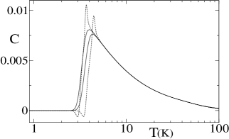
Figure 4: Average specific heat $C$ versus time $t$ in cooling from $T_{0}=100K$ (normal curve) to $T_{l}=0.9K$ and reheating (dashed curve), with two different cooling rates: $\omega=10^{-4}(Ks)^{-1}$ (curves on the left) and $\omega=10^{-3}(Ks)^{-1}$ (curves on the right). The probability of the disorder is given by (1) with $0\,K<\varepsilon<5\,K$ and $100{\rm\,K}<V<400{\rm\,K}$. $\gamma_{0}=10^{12}{\rm s}^{-1}$, as for experiments by A. Nittke et al. in review .

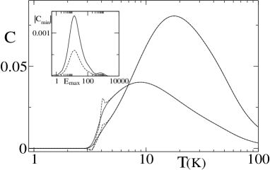
Figure 5: The same protocol as in Fig. 4, but with stronger disorder: $0{\rm\,K}<\varepsilon<20{\rm\,K}$ and $0{\rm\,K}<\varepsilon<40{\rm\,K}$ (larger curve); $\omega=10^{-3}(Ks)^{-1}$. In the insert the dependence of the minimum negative specific heat as a function of the width of the energy distribution is displayed for $100{\rm\,K}<V<400{\rm\,K}$ and $100{\rm\,K}<V<800{\rm\,K}$ (dashed line). $E_{min}=0$.

The negativity of $C_{h}$ shows that the quasi-stationary state of the TLS cannot be viewed as effective equilibrium, as far as the reheating is concerned. In order to make the meaning of this result more clear, we note that in the slow limit, where one decreases $|\sigma|$ and simultaneously increases the time $T$ remains constant, we expect convergence to equilibrium. Indeed, the temperature region where $C_{h}$ is negative, shrinks to zero as $\sim\ln(1/|\sigma|)$ [see (8)], but the magnitude of the negative minimal value of $C_{h}$ in this region does not depend much on $\sigma$. This is seen upon plotting $C_{h}$ versus $x/\sigma=\sigma^{-1}\exp(-V/T)$; see Fig. 3. However the negativity of $C_{h}$, and the very difference between $C_{h}$ and $C_{c}$, is sensitive to the values $\varepsilon$ and $V$ of the single-system motion.

Thus, upon averaging over the disorder —as given by (1) with experimental values for the parameters of $P(\varepsilon,V)$— the single-system memory effects gradually disappear; see Figs. 4, 5. Even though each TLS remains non-equilibrium, $C_{h}$ tends to $C_{c}$ eliminating the difference between cooling and heating. The same holds for the energy $\varepsilon n$.

We shall now discuss another method for displaying this non-equilibrium feature. In contrast to the above features which are essentially single-system and tend to disappear in the presence of disorder, the new method is based on the presence of an ensemble.

Temperature shift protocol. Motivated by Kovacs experiment kovacs , we perform the following protocol:

1. Consider an ensemble of non-interacting TLSs characterized by a distribution $P(\varepsilon,V)$. The ensemble is equilibrated at a given high temperature $T_{0}$.

2. Between times $t=0$ and $t_{c}$ the bath is cooled down following (4). The cooling is terminated at a low temperature $T_{l}$ so that the ensemble averaged energy $\langle\varepsilon n\rangle\equiv\int\varepsilon\,{\rm d}\varepsilon\,{\rm d}V\,P(\varepsilon,V)n(\varepsilon,V)$ reached a stationary value. This determines the time $t_{c}$. Note that $\langle\varepsilon n\rangle$ is observable in experiments using, e.g., heat release measurements review . Now $\langle\varepsilon n\rangle$ equals its equilibrium value:

$$\langle\varepsilon\,n\rangle|_{t=t_{c}}=\left\langle\varepsilon\,[\,e^{\beta_{f}\varepsilon}+1\,]^{-1}\right\rangle\equiv\langle\varepsilon\,n_{eq}\rangle.$$ (11)

This condition defines the temperature $T_{f}=1/\beta_{f}$. If most of the TLSs in the ensemble happen to be described at $t=t_{c}$ by a single temperature, then this temperature will be close to $T_{f}$ by definition. $T_{f}$ turns out to be of the same order of the average freezing temperature $\langle T^{*}\rangle$.

3. We want to monitor to what extent the state of the ensemble at $t=t_{c}$ is really close to some internal equilibrium. To this end, the bath temperature is suddenly switched to $T_{f}$, and the resulting evolution of $\langle\varepsilon n\rangle$ is monitored. Due to the sudden switching, the evolution is obtained averaging Eq. (3) at the bath temperature $T_{f}$, and with initial state (11):

$$\Delta\varepsilon\equiv\langle\varepsilon n_{t}\rangle-\langle\varepsilon n_{eq}\rangle=\langle\varepsilon e^{-\frac{t-t_{c}}{\tau}}(n-1/(e^{\beta_{f}\varepsilon}+1))\rangle.$$ (12)

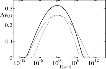
Figure 6: $\Delta\varepsilon$ versus time $t$ for the disordered ensemble with probability distribution given by (1). The cooling protocol (4) started from $T_{0}=100{\rm\,K}$ to $T_{l}=3K$, with $\omega=10^{-3}\,({\rm\,K}{\rm s})^{-1}$. Thick curve (stronger disorder): $0{\rm\,K}<\varepsilon<100{\rm\,K}$, $100{\rm\,K}<V<800{\rm\,K}$, $T_{f}=16.6{\rm\,K}$. Normal curve: $0{\rm\,K}<\varepsilon<50{\rm\,K}$, $100{\rm\,K}<V<800{\rm\,K}$ $T_{f}=15.3{\rm K}$. Dashed curve (weaker disorder): $0{\rm\,K}<\varepsilon<50{\rm\,K}$, $100{\rm\,K}<V<400{\rm\,K}$, $T_{f}=8.8{\rm\,K}$.

It is seen from (12) that by our construction $\Delta\varepsilon$ should be zero both at $t=t_{c}$ and for a very large $t-t_{c}$. It will stay zero for all times $t>t_{c}$, if the state of (almost) each TLS in the ensemble is described by the same temperature (which need not be equal to that of the bath). Yet another case, where $\Delta\varepsilon$ is constant for $t>t_{c}$ is when there is no disorder in the ensemble. Thus, the change of $\Delta\varepsilon$ depends both on the disorder and on a non-equilibrium state at $t=t_{c}$. The behavior of $\Delta\varepsilon$ for experimentally meaningful parameters is shown in Fig. 6. Since the change of $\Delta\varepsilon(t)$ is finite, a sizable fraction of the ensemble is at $t=t_{c}$ far from a local equilibrium. To gain more understanding, consider the simplest ensemble, which is an equal-weight mixture of two TLSs with parameters $(\varepsilon_{1},V_{1})$ and $(\varepsilon_{2},V_{2})$. Eq. (12) implies

$$2\Delta\varepsilon=\varepsilon_{1}(e^{-\frac{t-t_{c}}{\tau_{1}}}-e^{-\frac{t-t_{c}}{\tau_{2}}})[\,n(\varepsilon_{1},V_{1})-1/(e^{\beta_{f}\varepsilon_{1}}+1)],$$

where $\tau_{i}=\exp(\beta_{f}V_{i})/[\gamma_{0}(1+\exp(-\beta_{f}\varepsilon_{i}))]$ for $i=1,2$ are the relaxation times (see (3)), $n(\varepsilon_{1},V_{1})$ is given by (9), and where the temperature $\beta_{f}$ is defined as in (11) summing over the two TLSs ensemble. For the considered simplest ensemble, $\Delta\varepsilon$ is positive for $t>t_{c}$. This is because the slowest system—e.g., system $1$, if $\tau_{1}>\tau_{2}$—has its non-equilibrium upper-level probability $n(\varepsilon_{1},V_{1})$ larger than the final equilibrium one $[e^{\beta_{f}\varepsilon_{1}}+1]^{-1}$. In other words, the slowest system is further from the equilibrium. The behavior of $\Delta\varepsilon(t)$ for an experimentally relevant disorder distributions (1) is displayed in Fig. 6. The fact that $\varepsilon(t)\geq 0$ implies the same explanation as above: the slow TLSs are further from equilibrium. Two important (and for the present effect general) facts seen in Fig. 6 is that the stronger disorder leads to i) larger value of $T_{f}$ and ii) larger maximum of $\Delta\varepsilon$.

In conclusion, we studied memory effects in the Standard Model for glasses. This model, besides describing low-temperature properties of many amorphous materials review , has important applications in NMR and protein physics frau . It is known from previous works huang ; amjp that when a single TLS is cooled down to low temperatures, the relaxation increases due to impeding of the thermal activation, and the system appears in a quasi-stationary, non-equilibrium state. In contrast to equilibrium, this state depends on the detailed features of the relaxation, such as the barrier height or the cooling rate and upon reheating manifests itself via a negative specific heat amjp .

We confirmed the latter results by showing that the negative magnitude of the reheating specific heat is almost insensitive to the decreasing of the cooling-reheating rate. Next we showed that the single-particle non-equilibrium (memory) effects disappear for a disordered ensemble. Since only the latter is experimentally meaningful, one should question whether the single-particle memory effects can be observed at all. Our main result is that motivated by Kovacs experiments in kovacs , we designed a protocol which is able to reflect the non-equilibrium features of a disordered ensemble. The effect is sensitive to the details of the disorder and, if realized experimentally, it can assess the consistency of the model. We have also found two universal features of the effect: i) it is more visible for a stronger disorder and ii) its sign is determined by the fact that slower elements of the ensemble are further from equilibrium.

A.E.A. was supported by Volkswagenstiftung and partially by FOM/NWO.

References

- (1) P.W. Anderson, B.I. Halperin and C. M. Varma, Phil. Mag. 25, 1 (1972). W. A. Phillips, J. Low. Temp. Phys. 7, 351 (1972).
- (2) Tunnelling Systems in Amorphous and Crystalline Solids, ed. by P.Esquinazi (Springer-Verlag Berlin, 1998).
- (3) H. Frauenfelder et al., Rev. Mod. Phys. 71, S419 (1999).
- (4) A. J. Kovacs, Adv. Polym. Sci. 3, 394, (1963).
- (5) L. Berthier and J-P. Bouchaud, Phys Rev. B 66, 054404 (2002); L. F. Cugliandolo, G. Lozano and H. Lozza, Eur. Phys. J. B 41, 87 (2004); S. Mossa and F. Sciortino, Phys Rev. Lett. 92, 045504 (2004); G. Aquino , L. Leuzzi and T. M. Nieuwenhuizen, Phys. Rev. B 73, 094205 (2006)
- (6) M. Huang and J.P. Sethna, Phys. Rev. B 43, 3245 (1991). J.J. Brey and A. Prados, Phys. Rev. B 43, 8350 (1991). D.A. Parshin and A. Wurger, Phys. Rev. B 46, 762 (1992).
- (7) J. Bisquert, Am. J. Phys. 73 (2005).