\title{Entropy, dimension, and state mixing in a class of time-delayed
dynamical systems}
\author{D. J. Albers}
\email{albers@cse.ucdavis.edu}
\affiliation{Max Plank Institute for Mathematics in the Sciences,
Leipzig 04103, Germany}

\author{Fatihcan M. Atay}
\email{atay@member.ams.org}
\affiliation{Max Plank Institute for Mathematics in the Sciences,
Leipzig 04103, Germany}

\date{\today}
\keywords{Chaos, high dimensions, structural stability,
Lyapunov exponents, delay, entropy,
Kaplan-Yorke dimension}
\pacs{05.45.-a, 89.75.-k, 05.45.Tp, 02.30.Ks, 05.45.Jn, 05.45.Pq}

\begin{abstract}%
  Time-delay systems are, in many ways, a natural set of dynamical
  systems for natural scientists to study because they form an
  interface between abstract mathematics and data. However, they are
  complicated because past states must be sensibly incorporated into
  the dynamical system. The primary goal of this paper is to begin to
  isolate and understand the effects of adding time-delay coordinates
  to a dynamical system. The key results include (i) an analytical
  understanding regarding extreme points of a time-delay dynamical
  system framework including an invariance of entropy and the variance
  of the Kaplan-Yorke formula with simple time re-scalings; (ii)
  computational results from a time-delay mapping that forms a path
  between dynamical systems dependent upon the most distant and the
  most recent past; (iii) the observation that non-trivial mixing of
  past states can lead to high-dimensional, high-entropy dynamics that
  are not easily reduced to low-dimensional dynamical systems; (iv)
  the observed phase transition (bifurcation) between low-dimensional,
  reducible dynamics and high or infinite-dimensional dynamics; and
  (v) a convergent scaling of the distribution of Lyapunov exponents,
  suggesting that the infinite limit of delay coordinates in systems
  such are the ones we study will result in a continuous or (dense) point
  spectrum.%
\end{abstract}%

\maketitle

I Introduction

Experimental, scientific data for which time is an independent parameter is collected in the form of a scalar or vector time-series. The vector time-series rarely measures all of the independent coordinates required for a full specification of the system; the scalar time-series data never will. Nevertheless, that even a scalar time-series can be used to represent and reconstruct the original dynamical or natural system from which the data originated was a problem addressed well by Takens takensstit , Packard et al. geo_of_time_series , and Sauer et al. embedology . That there exist mappings that can reconstruct the dynamical system from observed time-series has also been shown (e.g., Hornik et al. hor2 ), even if the actual reconstruction has proven difficult sprott_book ; kantz_book . Nevertheless, it is usually time-delay dynamical systems that are of prime interest for practical analysis of natural systems because they are often the dynamical systems closest to real data. In this paper, we study discrete-time dynamical systems wth time delays. There are, of course, many formulations of time-delay dynamical systems; we wish to target and isolate the effects associated with adding time-delay coordinates using the simplest possible construction (for an alternative, see manffra_kantz , doyne_dds , or clint_dde ). To achieve this end, we have structured this paper so as to study various extremes that are complimented with results for intermediate cases. In particular, we consider the dynamics of an iterated map and its mixing with a single delay from the distant past. Moreover, to isolate and demonstrate the diversity among the different mappings, we consider two maps whose parameter spaces are diametrically opposed — the logistic map, which has dense stable periodic orbits for positive parameter values for which it remains bounded; and the tent map, which has a unique Sinai-Ruelle-Bowen (SRB) measure youngSRB over a large portion of its parameter space. It is worth noting that despite this difference, these maps are conjugate to one another at least one parameter value. A fundamental computational analysis of delay dynamical systems as they are used to approximate delay differential equations, and the characteristics of the diagnostics we will also study is presented in Ref. doyne_dds , which provides the best computational background for the study we will present in this paper.

We begin introducing time-delay systems in section II and the associated diagnostics in section III. With this groundwork laid, we begin the analysis in section IV with an analytical study of both the dynamics and the diagnostics of two extremes — (scalar) mappings dependent only on the most recent time-step and mappings dependent only on a single time-step from the distant past. Said differently, we study the dynamics and isolate the effects on various standard diagnostics of a simple time-rescaling where there is no mixing of states at different times. While we will claim some circumstances where the delay dynamical systems we study approximate infinite-dimensional, continuous spectrum systems, we are also interested in isolating the effects of rescaling time and adding delay coordinates. In the circumstance when time is rescaled, we show that the metric entropy is invariant to the time-rescaling, the largest Lyapunov exponent follows a simple rescaling that is a function of the time-delay, and the Kaplan-Yorke dimension formula can produce deceiving results. (It is known that as the delay is increased, Kaplan-Yorke dimension increases linearly; we will provide insight into why this is so.) The section V intermediate cases follow via a computational study that forms a bridge between the normal and the time-rescaled maps. As past states are mixed, for similar reasons that allow for the time-series embedding theorems to function, the dynamics become much more complicated and are not easily reduced to low-dimensional dynamical systems. Moreover, as the states are mixed, the results can depend on the parity of the number of delays and often depend profoundly on the chosen map. Aside from studying the effects of adding delay coordinates, it will also prove important to study the variation that exists over different explicit mappings. To isolate the effects of adding delays from the effects dependent on a particular mapping, we consider, as previously mentioned, two practical extrema among mappings — the tent and logistic maps. These maps represent “functional extrema” in the sense that the tent map has a unique SRB measure for a large, hole-free, open set of parameter values; whereas the logistic map has stable, hyperbolic, periodic dynamics for a dense set of parameter values graczyk_paper . Thus, the tent map is extremely dynamically stable in the sense that chaotic dynamics is maintained when parameters are changed. This is in contrast to the logistic map which, upon parameter variation, bears witness to catastrophic changes in dynamical behavior realized via the dense stable periodic orbit structure in parameter space. Nevertheless, we will observe that adding time-delays decreases, in a broad sense, the existence of periodic windows even for maps that have dense stable periodic windows in their parameter space. Moreover, high-entropy, high-dimensional geometric structure is observed for non-trivial mixing of previous states.

II Framework

We address issues related to dynamical systems where the present (time-delay-vector) state

$$\mathbf{x}_{t}=(x_{t},x_{t-1},x_{t-2},\cdots,x_{t-\tau})$$

is dependent upon past states with mappings of the form:

$$\mathbf{x}_{t+1} =\mathbf{F}(\mathbf{x_{t}})$$

$$=(F(x_{t},\dots,x_{t-\tau}),x_{t},x_{t-1},\cdots,x_{t-\tau+1})$$

where $\mathbf{F},F\in C^{r}$ ($r>0$), $\tau\in\mathbb{N}$, $\mathbf{x_{t}}\in\mathbb{R}^{\tau+1}$, and $x_{t}\in\mathbb{R}$ is always bounded. There exist an infinite number of ways to combine current and previous states, for instance by a simple summation of previous states represented by:

$$x_{t+1}=F(x_{t},\dots,x_{t-\tau})=\sum_{i=0}^{\tau}\beta_{i}f_{i}(x_{t-i})$$ (1)

where $\beta_{i}\in\mathbb{R}$ and $f\in C^{r}$ ($r>0$). One can further restrict to the case where $f_{i}$ is identical for all $i$. One nontrivial example worth mentioning where the $f_{i}$’s are not identical, but where $F$ remains a linear combination of previous states, is the standard delayed feedback case which can be arrived at by setting $f_{0}$ to a $C^{r}$ map, $(1-\beta_{\tau})f$, and $f_{\tau}=\beta_{\tau}x_{\tau}$ (see logistic_delayed_feedback for more information on this particular formulation). Note that all of the above time-delay dynamical systems are $d=\tau+1$ dimensional.

In this paper we concentrate on the case

$$x_{t+1}=(1-\beta)f(x_{t})+\beta f(x_{t-\tau})$$ (2)

for some given $f:\mathbb{R}\rightarrow\mathbb{R}$, where $\tau\in\mathbb{Z}^{+}$ is the time delay and the scalar $\beta\in[0,1]$ is a measure of the relative effect of the past on the evolution. With $\beta=0$ we have the evolution generated by the simple iteration rule

$$x_{t+1}=f(x_{t})$$ (3)

which corresponds to the standard map with no delays (ND), whereas when $\beta=1$ we obtain what we will call a pure delay (PD) system

$$x_{t+1}=f(x_{t-\tau}).$$ (4)

A primary question we will address is the nature of the change in dynamics of (2) between these two extreme (ND and PD) cases as $\beta$ is varied. For $\beta\in(0,1),$ (2) has a $(\tau+1)$-dimensional state space in the coordinates $\mathbf{x}_{t}=(x_{t},x_{t-1},\dots,x_{t-\tau}),$ so it is convenient to view also the extreme cases as $(\tau+1)$-dimensional. The system (2) thus provides a simple background for investigating the effect of past information on the dynamics.

An important motivation for studying the system (2) comes from synchronization of networks. Indeed, the so-called coupled map lattice Kaneko-book93 in the presence of transmission delays takes the form Atay-PRL04

$$x_{t+1}^{i}=f(x_{t}^{i})+\frac{\beta}{k_{i}}\sum a_{ij}(f(x_{t-\tau}^{j})-f(x_{t}^{i})),\qquad i=1,\dots,N.$$ (5)

Here $x_{t}^{i}$ is the state at time $t$ of the $i$th member (node) of a network of $N$ coupled dynamical systems, each of which follows the evolution rule (3) in isolation, but interacts with its neighbors when coupled to the network. The scalar $\beta$ represents the coupling strength. The scalars $a_{ij}$ are 1 whenever $i$ and $j$ are neighbors and zero otherwise, and $k_{i}=\sum_{j}a_{ij}$ is the degree of node $i$, i.e., its number of neighbors. The nonnegative integer $\tau$ represents the time delay in the information transmission between the neighbors of the network. It has been shown that the system (5) can synchronize, i.e., $|x_{t}^{i}-x_{t}^{j}|\rightarrow 0$ as $t\rightarrow\infty$ for all $i,j$, even in the presence of a positive transmission delay Atay-PRL04 . Then (5) asymptotically approaches a synchronous solution where $x_{t}^{i}=x_{t}$ for all $i$. It is easy to see then that the synchronous solution $x_{t}$ satisfies (2). In other words, (2) describes the dynamics of the synchronous solutions of coupled map lattices in the presence of transmission delays. It has been shown that the presence of delays greatly enriches the synchronous dynamics, whereas in the undelayed case the dynamics of the synchronized network and the isolated units are identical Atay-PRL04 ; Atay-Complexity04 . We investigate further aspects of this observation in the following sections.

III Diagnostics

The primary diagnostic quantities we will use in this paper are the Lyapunov characterisctic exponents (LCE) and quantities defined by the Lyapunov spectrum, such as the metric entropy $h_{\mu}$ and the Kaplan-Yorke dimension, $D_{KY}$ pesinlebook ; shimnag . Recall that each Lyapunov exponent in the Lyapunov spectrum is given by:

$$\chi_{j}=\lim_{t\rightarrow\infty}\frac{1}{t}\ln\|((D\mathbf{F}^{t})^{\top}(D\mathbf{F}^{t}))^{1/2}\cdot v_{j}\|$$ (6)

where $(D\mathbf{F}^{t})^{\top}$ is the transpose of the Jacobian $D\mathbf{F}^{t}$ and $v_{j}$ is a basis element of the tangent space (i.e., there are $d$, $d$-dimensional, mutually orthogonal vectors, each of which correspond to basis elements of the tangent space; for more information, see pesinlebook ; ruellehilbert ; guck ). For convenience, we will assume that the Lyapunov exponents are monotonically ordered by index according to $\chi_{i}\geq\chi_{i+1}$. In this work, we utilize the standard algorithm for computing the LCEs numerically as is given in Benettin et al. benn2 or Shimada and Nagashima shimnag . Furthermore, the metric entropy is given by the sum of the positive LCEs,

$$h_{\mu}=\sum_{\chi_{i}>0}\chi_{i}.$$ (7)

Similarly, the Kaplan-Yorke dimension of an attractor Kaplanyorke ; kaplan_yorke_2 is given by:

$$D_{KY}=j+\frac{\chi_{d}+\dots+\chi_{d-j}}{|\chi_{d-j-1}|}$$ (8)

where $j<d$ is the largest integer such that $\chi_{d}+\dots+\chi_{d-j}\geq 0$.

IV Effects of a pure delay-time rescaling

The ND and PD cases represent the extrema of Eq. (1) relative to the $\beta$ parameters; thus, an understanding of both the trivial and PD cases will form a foundation for studying Eq. (1) and, in particular, Eq. (2). In this special case the LCE scalings with $d$ can be handled analytically. Thus, the following results apply for $f\in C^{r}$ ($r\geq 1$), assuming that $f$ supports a unique SRB measure youngSRB or has robust chaos yorkerobustchaos ; unimodalrobust (thus, these results are largely independent of a particular choice of $f$).

Lemma 1 (Lyapunov spectrum for PD)

The Lyapunov spectrum of (4) is

$$\chi_{1}=\chi_{2}=\cdots=\chi_{\tau+1}=\frac{\mu}{\tau+1},$$ (9)

where $\mu$ is the Lyapunov exponent of $f$.

Proof. Defining the vector $\mathbf{x}_{t}=(x_{t},x_{t-1},\dots,x_{t-\tau})\in\mathbb{R}^{\tau+1}$, we write (4) in vector form

$$\mathbf{x}_{t+1}=(f(x_{t-\tau}),x_{t},\dots,x_{t-\tau+1}).$$ (10)

It follows that

$$\mathbf{x}_{t+\tau+1} =(x_{t+\tau+1},x_{t+\tau},\dots,x_{t+1})$$

$$=(f(x_{t}),f(x_{t-1}),\dots,f(x_{t-\tau})).$$

Rescaling time as

$$s=\frac{t}{\tau+1}$$ (11)

gives

$$(x_{(\tau+1)s+(\tau+1)},x_{(\tau+1)s+\tau},\dots,x_{(\tau+1)s+1})$$

$$=(f(x_{(\tau+1)s}),f(x_{(\tau+1)s-1}),\dots,f(x_{(\tau+1)s-\tau}))$$

Finally letting $u_{s}^{i}=x_{(\tau+1)s-(i-1)}$ for $i=1,\dots,\tau+1$, we obtain

$$(u_{s+1}^{1},u_{s+1}^{2},\dots,u_{s+1}^{\tau+1})=(f(u_{s}^{1}),f(u_{s}^{2}),\dots,f(u_{s}^{\tau+1})).$$

The last equation describes $\tau+1$ decoupled scalar systems each of which evolves by the identical rule of the form (3); so it has $\tau+1$ identical Lyapunov exponents. In view of the applied time scaling (11), it follows that the Lyapunov exponents of (10) are given by (9).

From Lemma 1 and Eq. (7), the following corollary is immediate.

Corollary 1 (Metric entropy invariant to a PD)

The standard metric entropy $h_{\mu}$ for the pure delay system (4) is independent of $\tau$.

On the other hand, Lemma 1 and Eq. (8) imply that the Kaplan-Yorke dimension is $D_{KY}=d=\tau+1$, which yields the following.

Corollary 2 ($D_{KY}$ is not invariant to a PD)

The Kaplan-Yorke dimension formula is not invariant to $\tau$ in the pure delay system (4).

Why is Corollary 2 important? The pure delay system (4) is equivalent to the non-scaled system (3) in every way but the calculated dimension. Moreover, for the PD system the “dimension” scales linearly with the delay. As we will see, for (2) also, $D_{KY}\approx d$ persists for $\beta$ being a significant distance from one, and only decreases as $\beta$ approaches one-half. But, as we will see, as $\beta$ is decreased from one or increased from zero, a significant change in the dynamics, as quantified by the invariant density and the structure of the LCEs, remains undetected in the dimension calculations. In particular, we will see a transition between the trivial high-dimensional dynamics of the PD that is easily reducible, and an irreducible manifestation of high-dimensional dynamics with no significant impact seen in $D_{KY}$ versus $\beta$. Thus, we claim that $D_{KY}$, and several other dimension estimates, can yield deceiving results for some time-delay dynamical systems because the $D_{KY}$ has an implicit coordinate dependence.

Summarizing, in dynamical systems with a PD that has no mixing of states for different times, the largest LCE is decreased by the factor that time has been rescaled, the metric entropy is invariant to the time-rescaling, and the Kaplan-Yorke dimension is equal to the factor by which time has been rescaled (i.e., $\tau+1$).

V Effects of state-mixing via added delay coordinates

With the endpoints ($\beta=0$ and 1) fully understood we can now begin to piece together the transitional region where states are mixed according to Eq. (2). At this time a full analytical understanding of this system is unavailable. Thus, for what follows, we will be restricted to a computational study. Moreover, as previously mentioned, these results, unlike those of the above section, will depend on the particular mapping; hence, the reason for an investigation using two common but dynamically distinct maps, the logistic and tent maps .

V.1 Tent map

We will begin the computational analysis with the standard tent map given by:

$$f(x)=\left\{\begin{array}[c]{ll}bx&\text{if $0<x\leq 1/2$},\\ b-bx&\text{if $1/2\leq x\leq 1$}.\end{array}\right.$$ (12)

at $b=2$. The first case we will consider is the tent map with $49$ delay coordinates ($d=50$) as this is a good intermediate value between the low-$d$ and high-$d$ cases. Considering Fig. 1, when $f$ is the standard tent map, there is little difference in the qualitative structure of the map for $d>4$; for $d>4$, all dimensional dependence and parity disappears (moreover, there do not exist periodic windows for $d>3$). Nevertheless, when $d<5$, there is significant dynamical variation as the parameters and the number of dimensions are changed. This dynamic variation includes the existence of periodic windows in the $\beta$-parameter space, dimension parity, and the lack of symmetry about $\beta=1/2$. This dimensional cutoff is likely related to the rate of decay of mutual information between $x_{t}$ and $x_{t-\tau}$; however, a precise understanding of this “functional” bifurcation is yet to be understood.

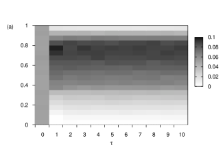
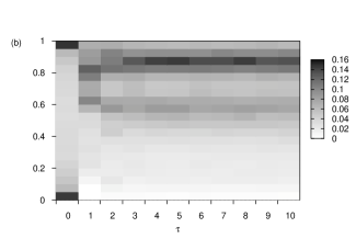
Figure 1: The dependence of the natural density for (2) on the delay $\tau$. (a) The tent map, (b) the logistic map. $\beta=0.8$.

Figure 2: Lyapunov exponents for (1) where $f$ is the standard tent map and $d=\tau+1=50$. The $\beta$ increments are $10^{-5}$, and for each $\beta$ the LCEs were calculated over $50000$ time-steps. The lower subfigure is a zoomed-out version that also shows the entropy plot.

Considering Fig. 2, for ease of description, let us parse the $\beta$ interval into three dynamical regions with monotonic ordering as $B_{1}=(0,0.3)$, $B_{2}=(0.3,0.7)$, and $B_{3}=(0.7,1)$. The first and third regions are transitions to “pure states,” where the dynamics correspond to dynamics of the original (tent) map with stochastic perturbations, or small perturbations of the invariant measure. This conclusion is drawn from two observations. First, given enough time-delays, the diagnostics ($h_{\mu}$ and the LCEs) in these regions make smooth transitions to their values for the pure states. Note that in region $B_{3}$ (Fig. 2), the LCEs (and thus the entropy and $D_{KY}$) behave in accordance with Lemma 1. The primary difference between regions one and three lies in the different LCE structure. Nevertheless, considering Fig. 3, the invariant densities of both region one and three are very similar (they are seemingly identical). Thus, the interpretation of the dynamics in regions one and three is of original map, $f$, perturbed by what is essentially (but not technically) noise. One final bit of support for the claim that regions one and three are dynamically similar is the observation that for $d>4$, the entropy (Fig. 2) and the invariant density (Fig. 3) are symmetric about $\beta=1/2$.

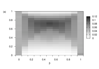
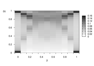
Figure 3: The natural density for (2) for (a) the tent and (b) the logistic maps with delay $\tau=50$. For values of $0\leq\beta\leq 1$, the vertical strips show the relative density of points in the interval $[0,1]$ for the evolution of (2), darker shades corresponding to higher density.

Region $B_{2}$, we believe, represents a fundamentally different kind of dynamics from the other regions. It is not a stochastically perturbed low-dimensional system, nor does it correspond to a transition to or from the pure states in regions $B_{1}$ or $B_{3}$. Instead, we claim, based originally on work by Manneville mann_lce_scaling (and a suggestion to the authors by Y. Kuramoto) that region $B_{2}$ is a representation of a continuous (LCE) spectrum, akin to a PDE. This hypothesis is driven by the qualitative difference in the dynamics that is indirectly witnessed via two qualitative observations. Considering the invariant density as depicted in Fig. 3, it is evident that the bifurcation that occurs between regions one/three and two leads to a significantly different invariant density than that of the perturbed map in regions one and three. This change in the invariant density suggests that there does exist a fundamental, qualitative difference between region two and regions one and three. That this qualitative change may be independent of dimension above a (soft) threshold can be seen in the invariance of the entropy. Considering Fig. 5, the entropy is, given $d$ high enough (e.g., $d>20$), largely invariant to increases in dimension. In particular, while the dimension is quadrupled, the change in entropy is less than $10$-percent and well below error estimates for the given number of iterations used in the numerical experiments. We assert that the variation in the entropy for $\beta>1/2$ is a numerical artifact of the errors in the smaller LCEs or the LCEs near zero.

Quantitative evidence of the existence of a continuous spectrum type behavior can be gained via a careful consideration of the LCEs as the dimension is increased. In particular, considering the plots in Fig. 4 where the LCE spectrum in region two is displayed for dimensions ranging from $d=50$ to $d=200$, normalized to $d=50$, the following observation is eminent: upon adding delays, the LCEs remain distributed in a relatively uniform way up to a time-rescaling. In fact, the primary difference in the plots at different dimensions is that $|\chi_{1}-\chi_{d}|$ decreases with dimension, and the intermediate LCEs are added in a manner consistent with their densities at lower $d$ as their numbers are increased. This statement can be quantified by considering the normalized distribution of positive LCEs. To achieve this, we begin by defining $M(\beta)$ as the number of positive LCEs at a given $\beta$. Next consider the distribution of LCEs, $\mathcal{D}$, via a discrete plot of $\chi_{i}$ versus $d(\frac{i(\chi_{i})}{M(\beta)})$ (the factor of $d$ normalizes $\mathcal{D}$ to unity). As can be seen in Fig. 6, there exists a universal scaling between LCEs that is invariant as $d$ is increased. Indeed the least squares fit of

$$d\frac{i(\chi_{i})}{M(\beta)}=\alpha e^{\gamma\chi_{i}}$$ (13)

for $d=50$ yields $\alpha=1.08,\gamma=-1.51$ (with a $\chi^{2}$-error of $0.978$) whereas for $d=200$, the fit yields $\alpha=1.02,\gamma=-1.59$ (with a $\chi^{2}$-error of $0.992$). These fits differ by less than five percent over a factor of four in dimension, and the fitting error decreases considerably with increasing dimension. That the LCEs remain relatively uniform (or are added in a manner consistent with their density for lower-$d$) up to a time rescaling and increase in dimension, implies that increasing the number of delays in this region is equivalent to increasing the resolution in a PDE-like mapping, leading to the conclusion that as $d\rightarrow\infty$, the LCE spectrum would tend to a continuous function at fixed $\beta$. If one accepts the proposition that the“law of large numbers cannot lie,” this LCE structure is a strong indication of an invariant (SRB) measure for a continuous-space system. (An exact qualification of this LCE structure is an object of future research).

The above reasoning leads us to conjecture that systems with LCE structure as is seen in $B_{2}$ corresponds to high-entropy, high-dimensional, equilibrium-like (possibly turbulent-like) systems that are not easily reduced or approximated by low-dimensional dynamical systems. Moreover, we believe that the dynamical characteristics are largely seen as a consequence of exactly the state mixing that allows the time-series embedding results to work correctly. It is also interesting that mixing states in some (non-trivial) circumstances can lead to a highly complicated, high-dimensional dynamical system. In this case, state mixing leads to higher-dimensional dynamics than the initial mapping (in this case the tent map). Finally, the dynamics in region $B_{2}$ can be identified as having bifurcation chains structure, which is defined for an interval of parameter space such that (i) the number of positive LCEs increases with increasing $d$ at a given parameter value, (ii) the Euclidean distance between sequential LCE magnitudes decreases with increasing $d$ at a given parameter value, (iii) the Euclidean distance between sequential LCEs remains relatively uniform at a given parameter value, and (iv) the LCEs cross zero transversally. Bifurcation chains structure represents a highly irreducible, high-dimensional dynamic type reminiscent of complex, equilibrium-like dynamics (such as homogeneous, fully developed fluid turbulence) — the bifurcation chains structure is discussed in detail (for a different system) in Refs. dynamicsPRL ; hypviolation .

That regions $B_{1}$ and $B_{3}$ consist of similar qualitative dynamics, and that these two regions are separated in $\beta$-space by region $B_{2}$ which has qualitatively different dynamics, implies that the transition between regions $B_{1}$ and $B_{2}$, and $B_{2}$ and $B_{3}$, represent a sort of bifurcation, or phase transition between “low-dimensional,” reducible dynamics and high-dimensional dynamics, irreducible dynamics. For the tent map, this phase transition is quite simple and void of highly complex structure. As we will see in the following section, this is likely due to the fact that the tent map has a nice absolutely continuous invariant measure over all the parameters we are considering.

Finally, while we refrain from a careful analysis of the dynamics at $\beta=1/2$, one is tempted to conjecture that this point represents a bifurcation behavior in parameter space. It is not only the midpoint of $B_{2}$ and thus a turning point of sorts in parameter space, but it is the point where $D_{KY}$ begins to drop from equality with $d$. Nevertheless, given that there is no change in the invariant density of at this point, the bifurcation will have to be characterized in a novel manner. It would not be surprising if a homogeneous function, renormalization style analysis could be performed at this point.

Figure 4: LCE plots of Eq. (1) where $f$ is the standard tent map restricted to region two ($B_{2}$) for dimensions ranging from $50$ to $200$ where the $d>50$ cases have been rescaled (by $d/50$) to the $d=50$ time-scale. The $\beta$ increments are $10^{-4}$, and for each $\beta$ the LCEs were calculated over $100000$ time-steps.

Figure 5: Metric entropy plots of Eq. (1) where $f$ is the standard tent map for dimensions ranging from $30$ to $200$. The $\beta$ increments are $10^{-4}$, and for each $\beta$ the LCEs were calculated over $100000$ time-steps.

Figure 6: The distribution of LCEs — $\chi_{i}$ versus $d\frac{i}{M(\beta)}$ — for Eq. (1) where $f$ is the standard tent map with dimensions $50$ and $200$ at fixed $\beta=1/2$.

V.2 Logistic map

We now take $f$ to be the standard logistic map given by:

$$f(x_{t})=ax_{t}(1-x_{t})$$ (14)

with $a=4$, the parameter setting for which the logistic map is absolutely continuous jakobson_abscontin and is conjugate to the tent map. Again, for ease of description, let us parse the $\beta$ interval into dynamical regions in monotonic ordering as follows: $B_{1}=(0,0.15)$, $B_{1\rightarrow 2}^{T}=(0.15,0.2)$, $B_{2}=(0.2,0.8)$, $B_{2\rightarrow 3}^{T}=(0.8,0.85)$, and $B_{3}=(0.85,1)$. These regions correspond to the case presented in Figs. 7 and 3 where $d$ is set to $50$. It is worth noting that both Figs. 1 and 7 display a dimension dependence that does not diminish by simply increasing $d$.

Figure 7: LCE plots of equation (1) where $f$ is the standard logistic map and $d=50$ (top two plots) and $d=51$ (bottom plot). The $\beta$ increments are $10^{-5}$, and for each $\beta$ the LCEs were calculated over $50000$ time-steps.

Just as was the case for the tent map, the first and third regions are transitions to “pure states,” where the dynamics correspond to dynamics of the original (logistic) map with stochastic perturbations, or small perturbations of the invariant measure. Again note that in region $B_{3}$ (Fig. 7), the LCEs (and thus the entropy and $D_{KY}$) behave as per Lemma 1. There is indeed little difference between the logistic and tent maps in these regions, which suggests that these regions will exist and be qualitatively the same for most stochastically stable ledrappier_young dynamical systems if $d$ is large enough. The dynamics seen in regions one and three is evidence that points to the logistic (for certain parameters) and tent maps being stochastically stable and satisfying L.-S. Young’s zero-noise limit youngSRB .

Region $B_{2}$ is most easily seen by considering either the invariant density in Fig. 3 (where the invariant density changes little between regions $B_{1\rightarrow 2}^{T}$ and $B_{2\rightarrow 3}^{T}$ yet is qualitatively distinct from regions $B_{1}$ and $B_{3})$, or the LCE spectrum in Fig. 7 where the bifurcation chains structure appears. Indeed, region $B_{2}$ is roughly the same for the logistic and tent maps, and we impart a similar interpretation of the dynamics. Nevertheless, there are important differences. For lower dimensions, the logistic map does display small periodic windows in region two, as can be seen in Fig. 8. The state mixing combined with added dimensions appears to have the effect of destroying the stable periodic orbits if $d$ is large enough — periodic orbits are observed for $d\leq 30$, whereas for $d\geq 50$, if they exist, they are below the $\beta$ resolution of $10^{-5}$. It is possible that the difference between the logistic and tent maps is a combination of the fact that the logistic map does not have persistent dynamics relative to parameter perturbations (i.e., the existence of dense, stable periodic orbits for $a\in[0,4]$) contrasted with the relative dynamical persistence of piecewise smooth maps yorkerobustchaos such as the tent map.

The $f$-dependence appears profoundly in the phase transition regions, $B_{1\rightarrow 2}^{T}$ and $B_{2\rightarrow 3}^{T}$. The structure of the transitional regions between the low-dimensional “pure states” and the high-dimensional dynamics of region $B_{2}$ are particular to the logistic map. In particular, both regions correspond to an effective value of the parameter $a_{\mathrm{eff}}\in(3.23,3.45)$ (where $a_{\mathrm{eff}}=\max\{\beta a,(1-\beta)a\}$), which corresponds to the region between the bifurcation from a fixed point to period two, but before the bifurcation from period two to period four, of the logistic map. The boundaries of these regions are roughly independent of magnitude of the dimension (as can be seen by considering the entropy versus dimension shown in Fig. 8), but these regions do have a dimension parity dependence. Assuming $d>4$, region $B_{2\rightarrow 3}^{T}$ is never a periodic window independent of the dimension parity. In contrast, region $B_{1\rightarrow 2}^{T}$ is not a periodic window when $d$ is odd but is always a periodic window when $d$ is even. Moreover, while the width of regions $B_{1\rightarrow 2}^{T}$ and $B_{2\rightarrow 3}^{T}$ are roughly equivalent and symmetric about $\beta_{\tau}=1/2$, they have different shapes and structures. This implies that if $\nu$ is a random variable with the invariant measure of $f(x_{t-\tau})$, both $f(x_{t})+\nu\neq f(x_{t}+\nu)$ and $f(x_{t})+\nu\neq f(x_{t-\tau})+\nu$, when $f$ is the logistic map. (In contrast to the logistic map, it appears that the time-ordering does not matter for the tent map.)

Figure 8: Entropy versus $\beta$ where $f$ is the standard logistic map with a varying number of delays.

VI Summary

Putting all the pieces together, for the time-delay systems (2) and (4), if the number of dimensions, $d=\tau+1$, is large enough, entropy remains roughly invariant to increases in $d$ while the LLE, the LCEs, and $D_{KY}$ do not. While the LLE and LCEs can still yield insight into the global structure of the attractor, many dimension calculations such as the Kaplan-Yorke dimension may yield deceiving results. We conjecture this is in general true for systems of the form (1), largely because dimension calculations have an implicit dimension- and thus coordinate dependence. Because of these issues, it is likely that diagnostics such as the metric entropy or the statistical complexity Crut88a , which are truly independent of coordinates, will be more useful for showing equivalence and difference in time-delay dynamical systems. Beyond the analysis of the diagnostics used to describe and investigate time-delay systems, we also demonstrated that both the time unscaled map with elements of the distant past and the time rescaled map with the elements of the current state produce roughly similar dynamics reminiscent of the $1$-d map plus noise. But, as the distant past and current states are mixed in more equal parts, the mixing of states only separated with time-delays can give rise to high-dimensional, irreducible, chaotic dynamics that we claim can approximate a PDE-like system if the mixing is via nearly equal contributions of states, and there exist enough degrees of freedom manifested as time-delays. Thus, we demonstrate two distinct classes of dynamics: one where the dynamics represent an infinite-dimensional system; and one where the dynamics represent a finite-dimensional system, with a phase transition (bifurcation) between the two dynamical classes, all in the simple context of mixing only two states of a single mapping. Moreover, this PDE-like dynamics produces a great deal of dynamic stability even for mappings that have a lot of periodicity without delays; thus the non-trivial state mixing can produce relatively stable chaotic dynamics over a sizable interval in parameter space. We hypothesize that this dynamic stability (persistence of chaos) occurs when the delay times allow for enough de-correlation between the active (non-zero) terms of Eq. (1) to mix states in a non-linear, but non-random-like manner. Nevertheless, the dynamics are dependent on the original maps that compose the time-delay. Finally, in dynamicsPRL and hypviolation , an example of bifurcation chains structure was presented that, relative to a measure on a function space, was persistent to parameter perturbations. Moreover, in these examples, in the presence of the bifurcation chains structure, the probability of periodic windows decreased as dimension increased. Here we observe similar results, but note that the bifurcation chains alone do not imply stability or lack of periodic windows as can be seen via the middle plot of Fig. 7.

D. J. Albers wishes to thank J. Dias, J. Jost, Y. Kuramoto, Y. Sato, C. R. Shalizi, J. C. Sprott, and U. Steinmetz for helpful discussions.

References

- [1] D. J. Albers and J. C. Sprott. Structural stability and hyperbolicity violation in high-dimensional dynamical systems. Nonlinearity, 19:1801–1847, 2006.
- [2] D. J. Albers, J. C. Sprott, and J. P. Crutchfield. Persistent chaos in high dimensions. Phys. Rev. E, 74:057201, 2006.
- [3] M. Andrecut and M. K. Ali. Robust chaos in smooth unimodal maps. Phys. Rev. E, 64:025203, 2001.
- [4] F. M. Atay and J. Jost. On the emergence of complex systems on the basis of the coordination of complex behaviors of their elements: Synchronization and complexity. Complexity, 10(1):17–22, 2004.
- [5] F. M. Atay, J. Jost, and A. Wende. Delays, connection topology, and synchronization of coupled chaotic maps. Phys. Rev. Lett., 92(14):144101, 2004.
- [6] S. Banerjee, J. A. Yorke, and C. Grebogi. Robust chaos. Phys. Rev. Lett., 80:3049–3052, 1998.
- [7] Luis Barreira and Ya. Pesin. Lyapunov exponents and smooth ergodic theory. AMS, 2002.
- [8] G. Benettin, L. Galgani, A. Giorgilli, and J-M. Strelcyn. Lyapunov characteristic exponents from smooth dynamical systems and for hamiltonian systems; a method for computing all of them. part 2: Numerical application. Meccanica, 15:21–30, 1979.
- [9] T. Buchner and J. J. Zebrowski. Logistic map with delayed feedback: Stability of a discrete-time-delay control of chaos. Phys. Rev. E, 63:016210, 2001.
- [10] J. P. Crutchfield and K. Young. Inferring statistical complexity. Phys. Rev. Let., 63:105–108, 1989.
- [11] J. D. Farmer. Chaotic attractors of an infinite-dimensional dynamical system. Physica D, 4:366–393, 1982.
- [12] P. Frederickson, J. L. Kaplan, E. D. Yorke, and J. A. Yorke. The Liapunov dimension of strange attractors. J. Diff. Eqn., 49:183–207, 1983.
- [13] J. Graxzyk and G. Światek. Generic hyperbolicity in the logistic family. Ann. of Math., 146:1–52, 1997.
- [14] J. Guckenheimer and P. Holmes. Nonlinear Oscillaions, Dynamical Systems, and Bifurcations of Vector Fields. Springer-Verlag, New York, 1983.
- [15] K. Hornik, M. Stinchocombe, and H. White. “Universal Approximation of an Unknown Mapping and its Derivatives Using Multilayer Feedforward Networks”. Neural Networks, 3:551, 1990.
- [16] M. Jakobson. Absolutely continuous invariant measures for one-parameter families of one-dimensional maps. Commun. Math. Phys., 81:39–88, 1981.
- [17] K. Kaneko, editor. Theory and applications of coupled map lattices. Wiley, New York, 1993.
- [18] H. Kantz and T. Schreiber. Nonlinear Time Series Analysis. Cambridge University Press, edition, 2003.
- [19] J. Kaplan and J. Yorke. Chaotic behavior of multidimensional difference equations, volume 730 of Lecture notes in mathemtics, pages 228–37. Springer-Verlag, 1979.
- [20] F. Ledrappier and L-S Young. The metric entropy of diffeomorphisms, Part I: Characterization of measures satisfying Pesin’s formula. Ann. of Math., 122:509–539, 1985.
- [21] E. F. Manffra, H. Kantz, and W. Just. Periodic orbits and topological entropy of delayed maps. Pys. Rev. E, 63:046203, 2001.
- [22] P. Manneville. Liapounov exponents for the Kuramoto-Sivashinsky model, volume 230 of Lect. N. Phys., page 319. Springer-Verlag, 1985.
- [23] N. Packard, J. Crutchfield, D. Farmer, and R. Shaw. Geometry from a time-series. Phys. Rev. Lett., 45:712, 1980.
- [24] D. Ruelle. Characteristic exponents and invariant manifolds in Hilbert space. Ann. of math., 115:243–290, 1982.
- [25] T. Sauer, J. Yorke, and M. Casdagli. Embedology. J. Stat. Phys., 65:579–616, 1991.
- [26] I. Shimada and T. Nagashima. A numerical approach to ergodic problems of dissapative dynamical systems. Prog. Theor. Phys., 61:1605–1635, 1979.
- [27] J. C. Sprott. A simple chaotic delay differential equation. Under review at Phys. Lett. A.
- [28] J. C. Sprott. Chaos and Time-series Analysis. Oxford University Press, 2003.
- [29] F. Takens. Detecting atrange attractors in turbulence. In D. Rand and L. Young, editors, Lecture Notes in Mathematics, volume 898, pages 366–381, Dynamical Systems and Turbulence, Warwick, 1981. Springer-Verlag, Berlin.
- [30] L-S Young. What are SRB measures, and which dynamical systems have them? J. Stat. Phys., 108:733–754, 2002.