On the use of Neumann’s principle for the calculation of the polarizability tensor of nanostructures

Abstract

The polarizability measures how the system responds to an applied electrical field. Computationally, there are many different ways to evaluate this tensorial quantity, some of which rely on the explicit use of the external perturbation and require several individual calculations to obtain the full tensor. In this work, we present some considerations about symmetry that allow us to take full advantage of Neumann’s principle and decrease the number of calculations required by these methods. We illustrate the approach with two examples, the use of the symmetries in real space and in spin space in the calculation of the electrical or the spin response.

I Introduction

The redistribution of electrons in a finite system that occurs when it is exposed to an external electromagnetic field is characterized by a set of constants called polarizabilitiespolarizability-book . The static polarizabilities refer to static fields, whereas the dynamical polarizabilities are functions of the frequency of the external field. Usually the name polarizability is restricted to the constants that determine the cited redistribution to first order in the applied field – when high-intensity fields are applied, one needs to make use of the higher-order ones or hyperpolarizabilities.

Besides characterizing the electromagnetic field-matter interaction, they are also important when studying collision phenomena, and as coarse indicators of physical size, structure and shape. The knowledge of the polarizability helps to obtain numerous physical quantities that depend on it: the dielectric constant and the refractive index of extended systems, the long-range interaction potentials between polarizable systems, van der Waals constants, etc. The dynamical polarizability, also, contains precious information about the excited states of a finite system: the peaks of the polarizability as a function of the energy determine the excitation energies of the system. The absorption cross section of a finite system is trivially related to the imaginary part of the dynamical polarizabilitypolarizability-book ; TDDFT . The oscillator strengths of the transition are the weights of the peaks of this absorption spectrum.

The polarizabilities may also be classified as dipole, quadrupole, etc., depending on the shape of the perturbing field: For example, the dipole polarizabilities characterize the response of the system to a dipole field. Rigorously speaking, one should also specify the physical magnitude that is measured, and speak, for example, of the dipole-dipole polarizability: the response of the system dipole to a dipole field. In this Article, we will exclusively deal with dipole-dipole first-order polarizabilities – the most commonly studied ones, and arguably the most important for nanostructure characterisation. Since there are three possible directions for the perturbing dipole field, and three possible directions for the system dipole response, the dipole-dipole polarizability is in fact a three-dimensional tensor.

Because of its tensorial character, one way of simplifying the calculation of the polarizability is to use Neumann’s principle neumann : the polarizability tensor of the system must be left invariant under any transformation that is also a point symmetry operation of the system. This condition of invariance reduces the number of independent tensor components, since it signifies relationships between those components, thus potentially reducing the number of calculations necessary to obtain the full tensor.

Numerous theoretical techniques can be used to calculate polarizabilities, with varying level of accuracy and detail. In particular, there is a class of methods that rely on the explicit use of the external perturbation, i.e. each line of the tensor is obtained by performing one calculation. Because of this, when using these methods it is not always obvious along which directions the perturbing fields should be aplied in order to make full use of Neumann’s principle. In this Article we discuss how this can be done.

Stricto sensu, the polarizabilities refer to the reaction to spin-independent (i.e., electrical) perturbations measured by spin-independent observables; they are referred to as density-density response functions. However, one can also think of more general response functions and apply spin-dependent perturbations and/or look at spin-dependent observables, obtaining in this way spin-density, density-spin and spin-spin response functions – these generalized objects are sometimes referred to as susceptibilities. Even though this work is mainly concerned with the polarizability itself, we will consider these more general objects, since we will also show how the calculation of the density-density and spin-spin response of a spin-saturated molecular system may be simplified.

In the following section, we recall the necessary definitions, and list some of the first-principles techniques that can be used to calculate polarizabilities of technologicaly relevant nano and bio structures – some of which can benefit from the simplifications proposed in this Article. These are discussed in Section III. Section IV shows how essentially the sames ideas may serve to simplify the calculation of the singlet and triplet excitations of systems whose ground-state is spin-saturated. Finally, we present two systems where the technique was used to compute the density-density and the spin-spin responses.

II The polarizability tensor

We will now introduce the notation and key quantities that are relevant for the use of symmetries to obtain the different linear response functions. Let $n_{\sigma}\;(\sigma=\uparrow,\downarrow)$ be the spin-density of a system of $N$ electrons:

$$n_{\sigma}(\vec{r},t)=\langle\Phi(t)|\sum_{k=1}^{N}\delta(\vec{r}-\hat{\vec{r}}_{k})\delta_{\sigma\sigma_{k}}|\Phi(t)\rangle\,,$$ (1)

If we apply an infinitesimal perturbation, $\delta v_{\sigma}(\vec{r},\omega)$ ($\sigma=\uparrow,\downarrow$), the response of the density, $\delta n_{\sigma}(\vec{r},t)=n_{\sigma}(\vec{r},t)-n_{\sigma}(\vec{r},0)$, will be related to the perturbation, to first order, by a density response function, $\chi$. In the frequency domain this is expressed as:

$$\delta n_{\sigma}(\vec{r},\omega)=\sum_{\sigma^{\prime}}\int\!\!\mathrm{d}^{3}r^{\prime}\,\chi_{\sigma\sigma^{\prime}}(\vec{r},\vec{r}^{\prime},\omega)\delta v_{\sigma^{\prime}}(\vec{r}^{\prime},\omega)\,.$$ (2)

The variation of the total density, $n=n_{\uparrow}+n_{\downarrow}$, and of the magnetization density, $m=n_{\uparrow}-n_{\downarrow}$, are given by:

$$\delta n(\vec{r},\omega) =\delta n_{\uparrow}(\vec{r},\omega)+\delta n_{\downarrow}(\vec{r},\omega)\,,$$ (3a)

$$\delta m(\vec{r},\omega) =\delta n_{\uparrow}(\vec{r},\omega)-\delta n_{\downarrow}(\vec{r},\omega)\,.$$ (3b)

After the system is perturbed, one can obtain information about the system by looking at the variation of some observable: $\delta\langle\hat{\mathcal{O}}\rangle(t)=\langle\hat{\mathcal{O}}\rangle(t)-\langle\hat{\mathcal{O}}\rangle(0)$. In our case, we will be looking at the dipole of the system in each of the spatial directions, $\hat{X}_{i}$. In order to learn about the spin modes, one may also look at $\hat{X}_{i}\hat{\sigma}_{z}$, where $\hat{\sigma}_{z}$ is the Pauli $z$-matrix. In the frequency domain, the behavior of these observables is given by:

$$\delta\langle\hat{X}_{i}\rangle(\omega) =\int\!\!\mathrm{d}^{3}r\,x_{i}\delta n(\vec{r},\omega)\,.$$ (4a)

$$\delta\langle\hat{X}_{i}\hat{\sigma}_{z}\rangle(\omega) =\int\!\!\mathrm{d}^{3}r\,x_{i}\delta m(\vec{r},\omega)\,.$$ (4b)

One also has to define which kind of perturbations are to be considered: We will restrict hereafter the formulation to dipole perturbations of two kinds:

(i) Spin-independent perturbations of the form:

$$\delta v^{[n]}_{\sigma}(\vec{r},\omega)=-x_{j}\kappa(\omega)\,.$$ (5)

In this case, the variations $\delta n$ and $\delta m$ are:

$$\delta n(\vec{r},\omega) =-\kappa(\omega)\int\!\!\mathrm{d}^{3}r^{\prime}\,\chi^{[nn]}(\vec{r},\vec{r}^{\prime},\omega)x^{\prime}_{j}\,,$$ (6a)

$$\delta m(\vec{r},\omega) =-\kappa(\omega)\int\!\!\mathrm{d}^{3}r^{\prime}\,\chi^{[mn]}(\vec{r},\vec{r}^{\prime},\omega)x^{\prime}_{j}\,,$$ (6b)

where we have defined the new objects:

$$\chi^{[nn]} =\chi_{\uparrow\uparrow}+\chi_{\uparrow\downarrow}+\chi_{\downarrow\uparrow}+\chi_{\downarrow\downarrow}$$ (7a)

$$\chi^{[mn]} =\chi_{\uparrow\uparrow}+\chi_{\uparrow\downarrow}-\chi_{\downarrow\uparrow}-\chi_{\downarrow\downarrow}$$ (7b)

The observables $\delta\langle\hat{X}_{i}\rangle(\omega)$ and $\delta\langle\hat{X}_{i}\hat{\sigma}_{z}\rangle(\omega)$ will be given by:

$$\delta\langle\hat{X}_{i}\rangle^{[n]}_{j}(\omega) =-\kappa(\omega)\int\!\!\!\int\!\!{\rm d}^{3}r\,{\rm d}^{3}r^{\prime}\,x_{i}\chi^{[nn]}(\vec{r},\vec{r}^{\prime},\omega)x^{\prime}_{j}\,,$$ (8a)

$$\delta\langle\hat{X}_{i}\hat{\sigma}_{z}\rangle^{[n]}_{j}(\omega) =-\kappa(\omega)\int\!\!\!\int\!\!{\rm d}^{3}r\,{\rm d}^{3}r^{\prime}\,x_{i}\chi^{[mn]}(\vec{r},\vec{r}^{\prime},\omega)x^{\prime}_{j}\,.$$ (8b)

The superscript “${[n]}$” means that the observable is measured after a spin-independent perturbation of the form given in Eq. (5) has been applied, whereas the subscript “$j$” means that this perturbation has been applied in the direction $j$.

(ii) Spin-dependent perturbations of the form:

$$\delta v^{[m]}_{\sigma}(\vec{r},\omega)=\left\{\begin{array}[]{r@{\quad,\quad}l}-x_{j}\kappa(\omega)&\sigma=\uparrow\\ x_{j}\kappa(\omega)&\sigma=\downarrow\,.\end{array}\right.$$ (9)

Or, making use of the Pauli $z$-matrix:

$$\delta v^{[m]}(\vec{r},\omega)=-x_{j}\kappa(\omega)\sigma_{z}\,.$$ (10)

The variations of $n(\vec{r},\omega)$ and $m(\vec{r},\omega)$ are:

$$\delta n(\vec{r},\omega) =-\kappa(\omega)\int\!\!\mathrm{d}^{3}r^{\prime}\,\chi^{[nm]}(\vec{r},\vec{r}^{\prime},\omega)x^{\prime}_{j}\,,$$ (11a)

$$\delta m(\vec{r},\omega) =-\kappa(\omega)\int\!\!\mathrm{d}^{3}r^{\prime}\,\chi^{[mm]}(\vec{r},\vec{r}^{\prime},\omega)x^{\prime}_{j}\,,$$ (11b)

with the definitions:

$$\chi^{[nm]} =\chi_{\uparrow\uparrow}-\chi_{\uparrow\downarrow}+\chi_{\downarrow\uparrow}-\chi_{\downarrow\downarrow}$$ (12a)

$$\chi^{[mm]} =\chi_{\uparrow\uparrow}-\chi_{\uparrow\downarrow}-\chi_{\downarrow\uparrow}+\chi_{\downarrow\downarrow}$$ (12b)

Now, the observables $\delta\langle\hat{X}_{i}\rangle(\omega)$ and $\delta\langle\hat{X}_{i}\hat{\sigma}_{z}\rangle(\omega)$ will be given by

$$\delta\langle\hat{X}_{i}\rangle^{[m]}_{j}(\omega) =-\kappa(\omega)\int\!\!\!\int\!\!{\rm d}^{3}r{\rm d}^{3}rx_{i}\chi^{[nm]}(\vec{r},\vec{r}^{\prime},\omega)x^{\prime}_{j}\,,$$ (13a)

$$\delta\langle\hat{X}_{i}\hat{\sigma}_{z}\rangle^{[m]}_{j}(\omega) =-\kappa(\omega)\int\!\!\!\int\!\!{\rm d}^{3}r{\rm d}^{3}rx_{i}\chi^{[mm]}(\vec{r},\vec{r}^{\prime},\omega)x^{\prime}_{j}\,.$$ (13b)

We now look at the quotients between the induced variations $\delta\langle\hat{X}_{i}\rangle(\omega)$ and $\delta\langle\hat{X}_{i}\hat{\sigma}_{z}\rangle(\omega)$ and the strength of the perturbation, $\kappa(\omega)$, for each one of the cases:

$$\alpha_{ij}^{[nn]}(\omega) =\frac{\delta\langle\hat{X}_{i}\rangle^{[n]}_{j}(\omega)}{\kappa(\omega)}$$ (14a)

$$\alpha_{ij}^{[mn]}(\omega) =\frac{\delta\langle\hat{X}_{i}\hat{\sigma}_{z}\rangle^{[n]}_{j}(\omega)}{\kappa(\omega)}$$ (14b)

$$\alpha_{ij}^{[nm]}(\omega) =\frac{\delta\langle\hat{X}_{i}\rangle^{[m]}_{j}(\omega)}{\kappa(\omega)}$$ (14c)

$$\alpha_{ij}^{[mm]}(\omega) =\frac{\delta\langle\hat{X}_{i}\hat{\sigma}_{z}\rangle^{[m]}_{j}(\omega)}{\kappa(\omega)}$$ (14d)

The usual definition of the polarizability refers to the first of these expressions, $\alpha_{ij}\equiv\alpha_{ij}^{[nn]}$. However, one may also be interested in the other kinds of responses. We will use the same notation ($\alpha$) for these response functions, although the name polarizability should be restricted for the first case. Another way of defining these functions is:

$$\alpha_{ij}^{\sigma\sigma^{\prime}}(\omega)=-\int\!\!\!\int\!\!{\rm d}^{3}r\,{\rm d}^{3}r^{\prime}\,x_{i}\chi_{\sigma\sigma^{\prime}}(\vec{r},\vec{r}^{\prime},\omega)x^{\prime}_{j}\,.$$ (15)

Obviously, the two definitions are related, and one may retrieve the $\alpha_{ij}^{[xy]}$ components from the $\alpha_{ij}^{\sigma\sigma^{\prime}}$ and viceversa:

$$\alpha_{ij}^{[nn]} =\alpha_{ij}^{\uparrow\uparrow}+\alpha_{ij}^{\uparrow\downarrow}+\alpha_{ij}^{\downarrow\uparrow}+\alpha_{ij}^{\downarrow\downarrow}$$ (16a)

$$\alpha_{ij}^{[mn]} =\alpha_{ij}^{\uparrow\uparrow}+\alpha_{ij}^{\uparrow\downarrow}-\alpha_{ij}^{\downarrow\uparrow}-\alpha_{ij}^{\downarrow\downarrow}$$ (16b)

$$\alpha_{ij}^{[nm]} =\alpha_{ij}^{\uparrow\uparrow}-\alpha_{ij}^{\uparrow\downarrow}+\alpha_{ij}^{\downarrow\uparrow}-\alpha_{ij}^{\downarrow\downarrow}$$ (16c)

$$\alpha_{ij}^{[mm]} =\alpha_{ij}^{\uparrow\uparrow}-\alpha_{ij}^{\uparrow\downarrow}-\alpha_{ij}^{\downarrow\uparrow}+\alpha_{ij}^{\downarrow\downarrow}$$ (16d)

Regarding its spatial structure – and thus dropping the spin indexes – the dynamical polarizability elements may be arranged in a second-rank 3x3 symmetric tensor $\boldsymbol{\alpha}(\omega)$. The absorption cross-section tensor is then simply proportional to its imaginary part:

$$\boldsymbol{\sigma}(\omega)=\frac{4\pi\omega}{c}\mathfrak{Im}\,\boldsymbol{\alpha}(\omega)\,,$$ (17)

where $c$ is the speed of light.

The static or the dynamical (hyper)polarizabilities can be calculated within different theoretical approaches. Our main concern here is (time-dependent) density functional theory – (TD)DFTTDDFT , but our arguments are quite general and apply equally well to other electronic structure methods. The simplest of these is perhaps obtaining the static (hyper)polarizabilities through finite differences, i.e., by applying small static electrical fields $\boldsymbol{E}_{j}$, and then calculating numerically the derivatives. On the other hand, the dynamical polarizability can be calculated through real-time propagation of the time-dependent Kohn-Sham equationsyabana . Moreover, both static and dynamical polarizabilities can be obtained through straighforward perturbation theory. In this case, “perturbation theory” refers to the application of Sternheimer equationsternheimer ; sternheimer4 in one way or another, either for the static or for the dynamicaltd-sternheimer ; Xavier case. Another very recent and quite promising approach, is a efficient Lanczos-based methodBaroni .

For all these methods the calculations rely on the explicit use of the external perturbation. If we want to calculate the full tensor, we have to perform three calculations, one for each spatial direction. If, moreover, we need both the density and spin modes, we have to make two calculations per spatial direction, one for each of the two possible perturbations discussed above. In the next sections we will show how the number of actual calculations can be severely reduced when using these methods by taking advantage of the symmetries of the system.

Note that the polarizability can also be obtained, for example, from the response functions, using, for example, the formalism developed by M. Casidacasida ; casida2 ; casida3 ; casida4 . This is a case in which the considerations presented below will not simplify the calculations, since they do not proceed by the successive application of the different perturbations.

III Spatial symmetries

In this section, we will drop the spin indices, since the whole argument is valid for any of the spin components of the polarizability.

By making use of Eq. (15), it is easy to prove that $\boldsymbol{\alpha}(\omega)$ is a proper tensor: If we consider a second orthonormal reference frame $\{\hat{e}^{\prime}_{1},\hat{e}^{\prime}_{2},\hat{e}^{\prime}_{3}\}$, $\boldsymbol{\alpha}(\omega)$ transforms following the tensorial transformation law:

$$\boldsymbol{\alpha}^{\prime}(\omega)=\mathbf{P}^{t}\boldsymbol{\alpha}(\omega)\mathbf{P}\,,$$ (18)

where $\boldsymbol{\alpha}^{\prime}(\omega)$ is the polarizability in the second reference frame, and $\mathbf{P}$ is the rotation matrix between the two frames.

This tensorial character of the polarizability permits us to work in any orthonormal reference frame; once we obtain its values, we may easily transform it by straightforward matrix manipulation. We may then choose the frame which is most appropriate, bearing in mind the geometry of the molecule, and this can reduce the total number of calculations. However, this liberty does not allow us to make full use of symmetry. For this purpose, we need to work with non-orthonormal directions.

Let us consider three linearly-independent, but possibly non-orthogonal, unit vectors $\{\hat{p}_{1},\hat{p}_{2},\hat{p}_{3}\}$. We define the polarizability elements $\tilde{\alpha}_{uv}(\omega)$ as:

$$\tilde{\alpha}_{uv}(\omega)=-\int\!\!\!\int\!\!{\rm d}^{3}r\,{\rm d}^{3}r^{\prime}\,(\vec{r}\cdot\hat{p}_{u})\chi(\vec{r},\vec{r}^{\prime},\omega)(\vec{r}^{\prime}\cdot\hat{p}_{v})\,.$$ (19)

This corresponds to a process in which the polarization of the perturbing field is along $\hat{p}_{v}$, and the dipole is measured along $\hat{p}_{u}$. If we know the 3x3 matrix $\tilde{\boldsymbol{\alpha}}(\omega)$, we get the real tensor $\boldsymbol{\alpha}(\omega)$ by making use of the following simple relationship, which can be obtained once again from Eq. (15):

$$\tilde{\boldsymbol{\alpha}}(\omega)=\mathbf{P}^{t}\boldsymbol{\alpha}(\omega)\mathbf{P}\,.$$ (20)

$\mathbf{P}$ is the transformation matrix between the original orthonormal reference frame and $\{\hat{p}_{1},\hat{p}_{2},\hat{p}_{3}\}$. Note that this transformation is in general not a rotation; $\mathbf{P}$ is not unitary. Moreover, no matter how familiar it looks, Eq. (20) is not a change of coordinates: $\tilde{\boldsymbol{\alpha}}(\omega)$ is not the polarizability tensor in the new reference frame. And finally, also note that the traces of $\tilde{\boldsymbol{\alpha}}$ and $\boldsymbol{\alpha}$ do not coincide:

$${\rm Tr}\left[\tilde{\boldsymbol{\alpha}}(\omega)\right]={\rm Tr}\left[\mathbf{P}^{t}\boldsymbol{\alpha}(\omega)\mathbf{P}\right]={\rm Tr}\left[\boldsymbol{\alpha}(\omega)\mathbf{P}\mathbf{P}^{t}\right]\,.$$ (21)

but $\mathbf{P}\mathbf{P}^{t}\neq\boldsymbol{1}$. Notwithstanding this, it tells us that we may obtain the polarizability tensor by calculating the related object $\tilde{\boldsymbol{\alpha}}(\omega)$.

Now let us assume that the molecule under study possesses some non-trivial symmetry transformations – to start with, we consider that it has two, $\mathcal{A}$ and $\mathcal{B}$. We consider an initial unit vector, $\hat{p}_{1}$, and define:

$$\hat{p}_{2}=\mathcal{A}\hat{p}_{1}$$

$$\hat{p}_{3}=\mathcal{B}\hat{p}_{2}$$ (22)

We assume that this may be done such that the set $\{\hat{p}_{1},\hat{p}_{2},\hat{p}_{3}\}$ is linearly independent.

We then perform a TDDFT calculation with the perturbing field polarized in the direction $\hat{p}_{1}$. This permits us to obtain the row $\{\tilde{\alpha}_{11},\tilde{\alpha}_{12},\tilde{\alpha}_{13}\}$. Since the matrix is symmetric, we also have the column $\{\tilde{\alpha}_{11},\tilde{\alpha}_{21},\tilde{\alpha}_{31}\}$. The symmetry of the molecule also permits us to obtain the diagonal: $\{\tilde{\alpha}_{33}=\tilde{\alpha}_{22}=\tilde{\alpha}_{11}\}$. The only missing element is $\tilde{\alpha}_{23}=\tilde{\alpha}_{32}$, but it is easy to prove that:

$$\tilde{\alpha}_{23}=\tilde{\alpha}_{1,\mathcal{A}^{-1}\hat{p}_{3}}\,,$$ (23)

which we can also get from our original calculation. The conclusion is that we have access to the full tensor by making only one calculation.

To fix ideas, we use the example of a molecule with one $n$-th order axis of symmetry ($n>2$). Let $\mathcal{R}$ be the rotation of $2\pi/n$ degrees around this axis. We then choose $\hat{p}_{1}$ not collinear with this axis, and also not perpendicular to it. If we define $\mathcal{R}\hat{p}_{1}=\hat{p}_{2}$ and $\mathcal{R}\hat{p}_{2}=\hat{p}_{3}$, the set $\{\hat{p}_{1},\hat{p}_{2},\hat{p}_{3}\}$ will be linearly independent. In this case, moreover, since $\mathcal{A}=\mathcal{B}=\mathcal{R}$, Eq. (23) reduces to $\tilde{\alpha}_{23}=\tilde{\alpha}_{12}$.

It may very well be that we may only find two linearly independent “equivalent axis”, $\hat{p}_{1}$ and $\hat{p}_{2}$, related by a symmetry transformation, $\mathcal{A}$ – this is the case of a system that possesses only a plane of symmetry, or only an axis of symmetry of order two. We may then define $\hat{p}_{1}$ to be a tilted vector with respect to this plane (not contained in it, and not perpendicular). Then, $\hat{p}_{2}=\mathcal{A}\hat{p}_{1}$, where $\mathcal{A}$ is the reflection on the plane, is an equivalent vector, and $\vec{p}_{3}$ can be chosen to lie in the symmetry plane (the obvious choice will be $\hat{p}_{3}=\hat{p}_{1}\wedge\hat{p}_{2}$, that ensures linear independence). We then only need two calculations, one with the polarization along $\hat{p}_{1}$ (or $\hat{p}_{2}$) and another with the polarization along $\hat{p}_{3}$. Moreover, if $\hat{p}_{1}$ is chosen to be tilted exactly $\pi/2$ with respect to the symmetry plane, the system of vectors is orthonormal, and we do not even need to apply Eq. (20). Note that this case applies to all planar molecules.

IV Singlet and triplet excitations in spin-saturated systems

We consider a system whose ground state is spin-saturated. It verifies:

$$\alpha_{ij}^{\uparrow\uparrow} =\alpha_{ij}^{\downarrow\downarrow}\,,$$ (24a)

$$\alpha_{ij}^{\uparrow\downarrow} =\alpha_{ij}^{\downarrow\uparrow}\,.$$ (24b)

And, in consequence, $\alpha_{ij}^{[nm]}=\alpha_{ij}^{[mn]}=0$, and

$$\alpha_{ij}^{[nn]} =2\alpha_{ij}^{\uparrow\uparrow}+2\alpha_{ij}^{\uparrow\downarrow}\,,$$ (25a)

$$\alpha_{ij}^{[mm]} =2\alpha_{ij}^{\uparrow\uparrow}-2\alpha_{ij}^{\uparrow\downarrow}\,.$$ (25b)

Despite this symmetry, in order to obtain all spin-components (which in this spin-saturated case are only two independent ones), by making use of the two types of perturbations defined in Eqs. (5) and (9), we would still need two calculations: one perturbing with a spin-independent potential – in order to obtain $\alpha_{ij}^{[nn]}$, and one with a spin-dependent one – in order to obtain $\alpha_{ij}^{[mm]}$.

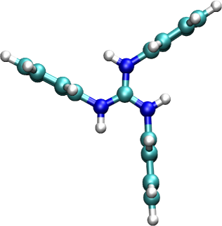
Figure 1: (Color online) Two different views of protonated triphenylguanidine (point group $C_{3h}$). In this picture, the dark blue atoms are nitrogen, the cyan represent carbon, and finally the white atoms are hydrogen.

However, one can easily use a similar scheme to the one outlined in the previous section in order to calculate the two polarizabilities in only one shot. The idea is to apply a perturbation in the form:

$$\delta v^{[\uparrow]}_{\sigma}(\vec{r},\omega)=\left\{\begin{array}[]{r@{\quad,\quad}l}-x_{j}\kappa(\omega)&\sigma=\uparrow\\ 0&\sigma=\downarrow\,,\end{array}\right.$$ (26)

or, in the Pauli matrix language:

$$\delta v^{[\uparrow]}(\vec{r},\omega)=-\frac{1}{2}\kappa(\omega)x_{j}(\hat{\sigma}_{0}+\hat{\sigma}_{z})\,.$$ (27)

It is then easy to verify that the response of the dipole observables will then be given by:

$$\delta\langle\hat{X}_{i}\rangle^{[\uparrow]}_{j}(\omega)=-\frac{1}{2}\kappa(\omega)\alpha_{ij}^{[nn]}\,,$$ (28a)

$$\delta\langle\hat{X}_{i}\hat{\sigma}_{z}\rangle^{[\uparrow]}_{j}(\omega)=-\frac{1}{2}\kappa(\omega)\alpha_{ij}^{[mm]}\,,$$ (28b)

thus providing us with the components of the two response functions that we need with only one calculation.

V Examples

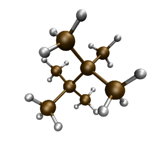
Figure 2: (Color online) One view of Si₈H₁₈ (point group $D_{3d}$). In this picture, the dark brown atoms are silicon and the grey atoms are hydrogen.

There are many complex molecules of tecnological relevance that present symmetries such that the schemes outlined in the previous sections can be used. We chose two of them to illustrated the method: protonated triphenylguanidine and one hidrogenated silicon cluster Si₈H₁₈. Triphenylguanidine compounds are regarded as interesting for quadratic nonlinear optical applications while hidrogenated silicon is an important optico-electronic material with potentially important technological applications.

The ground-state of protonated triphenylguanidine is spin-saturated, has one proper axis of symmetry of order three, one plane of symmetry, and one improper axis of rotation of order three (see Fig. 1). The ground-state of Si₈H₁₈ is spin-saturated, has an inversion center, one proper axis of symmetry of order three, three proper axis of symmetry of order two, three planes of symmetry, and one improper axis of symmetry of order six (see Fig. 2). This means one can make use of the schemes outlined in the previous sections to obtain all the components of the response functions with only one calculation: all components of both $\boldsymbol{\alpha}^{[nn]}(\omega)$ and $\boldsymbol{\alpha}^{[mm]}(\omega)$ tensors.

Without using the symmetry of the system the response functions were computed by applying spin-independent and spin-dependent perturbations from Eqs. (5) and (9) with polarization directions along the $x$, $y$ and $z$ directions. This way the response functions were straighforwardly obtained but required a total of six time-propagations.

To use the symmetry a set $\{\hat{p}_{1},\hat{p}_{2},\hat{p}_{3}\}$ is needed. In the case of protonated triphenylguanidine we built it by defining $\hat{p}_{1}$ to be a vector tilted $\pi/4$ with respect to the plane of symmetry and the two symmetry transformations $\mathcal{A}$ and $\mathcal{B}$ to be an inversion with respect to the plane and a $2\pi/3$ rotation around the axis of symmetry of order 3. In the case of Si₈H₁₈ we chose $\hat{p}_{1}$ to be a vector tilted $\pi/4$ with respect to the axis of symmetry of order three and both symmetry transformations $\mathcal{A}$ and $\mathcal{B}$ to be $2\pi/3$ rotations around the same axis.

Applying a perturbation of the same form as Eq. (26) with a polarization direction along $\hat{p}_{1}$ and using Eqs. (20), (28a) and (28b) allowed us to obtain the response functions with just one calculation in both cases.

All response calculations were done with the code octopus octopus using the Perdew-Zunger lda parametrization of the adiabatic local density approximation for the exchange-correlation potential. This method has already been successfully used for the calculation of optical spectra in a variety of systems, ranging from small moleculesmolecules and clustersc20 to biological systemsbio .

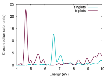
Figure 3: (Color online) Protonated triphenylguanidine averaged absorption cross-section for singlets and triplets. The curves obtained with and without the use of symmetry completely overlap.

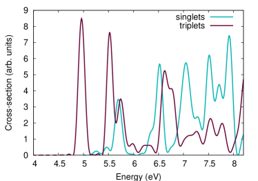
Figure 4: (Color online) Si₈H₁₈ averaged absorption cross-section for singlets and triplets. Again, The curves obtained with and without the use of symmetry completely overlap.

To represent the wave-functions in real space we used a uniform grid with a spacing of 0.195 Å and a box composed by spheres of radius 5 Å around every atom. In order to propagate the Kohn-Sham orbitals we employed state of the art algorithmspropagators . A time step of 0.0048 fs assured the stability of the time propagation, and a total propagation time of 19.35 fs allowed a resolution of about 0.1 eV in the resulting spectrum.

The results obtained are summarized in Fig. 3 and Fig. 4 where we plot the averaged absorption cross-section (trace of the tensor) for singlets and triplets.

VI Conclusions

In summary, we presented a scheme that can considerably reduce the number of calculations necessary to obtain the full polarizability tensor by using the symmetries of the system. These can be spatial symmetries (like planes of inversion or symmetry axis, e.g.) or they can lie in spin space (if the ground-state is spin saturated). Finally, the scheme is trivial to implement, and can be easily extended to different symmetries and different responses– i.e. higher multipole responses, and higher order hyperpolarizabilities –, so we expect that its usefulness to surpass the present context.

- (1) K. D. Bonin and V. Kresin, Electric-Dipole Polarizabilities of Atoms, Molecules and Clusters, (World Scientific, Singapore, 1997).
- (2) M. A. L. Marques and E. K. U. Gross, Annu. Rev. Phys. Chem. 55, 427 (2004); M. A. L. Marques, C. Ullrich, F. Nogueira, A. Rubio, K. Burke, and E. K. U. Gross (Eds.) Lecture Notes in Physics, Vol. 706 (Springer, Berlin, 2006)
- (3) F. E. Neumann, Vorlesungen über die Theorie der Elastizität der festen Körper und des Lichtäthers, B. G. Teubner-Verlag, Leipzig (1885).
- (4) K. Yabana and G. F. Bertsch, Phys. Rev. B 54, 4484 (1996).
- (5) R. M. Sternheimer, Phys. Rev. 96, 951 (1954); R. M. Sternheimer, ibid. 84, 244 (1951); R. M. Sternheimer and H. M. Foley, ibid. 92, 1460 (1953);
- (6) X. Gonze, J.-P. Vigneron, Phys. Rev. B 39, 13120-13128 (1989).
- (7) A. Dal Corso, F. Mauri, and A. Rubio, Phys. Rev. B 53, 15638-15642 (1996).
- (8) X. Andrade, S. Botti, M. A. L. Marques, and A. Rubio, to be published.
- (9) B. Walker, A. M. Saitta, R. Gebauer, and S. Baroni, Phys. Rev. Lett. 96, 113001 (2006).
- (10) M. E. Casida, in Recent Advances in Density Functional Methods, Part I, D. P. Chong (Ed.), page 155, World Scientific Press, Singapore (1995);
- (11) C. Jamorski, M. E. Casida, and D. R. Salahub, J. Chem. Phys. 104, 5134 (1996).
- (12) M. Petersilka, U. J. Gossmann, and E. K. U. Gross, Phys. Rev. Lett. 76, 1212 (1996).
- (13) T. Grabo, M. Petersilka, and E. K. U. Gross, J. Mol. Struct. (Theochem) 501, 353 (200).
- (14) M. A. L. Marques, A. Castro, G. F. Bertsch, and A. Rubio, Comput. Phys. Commun. 151, 60 (2003); A. Castro, H. Appel, M. Oliveira, C. A. Rozzi, X. Andrade, F. Lorenzen, M. A. L. Marques, E. K. U. Gross, and A. Rubio, Phys. Stat. Sol. B 243, 2465 (2006). http://www.tddft.org/programs/octopus/.
- (15) D. M. Ceperley and B. J. Alder, Phys. Rev. Lett. 45, 566 (1980); J. P. Perdew and A. Zunger, Phys. Rev. B 23, 5048 (1981).
- (16) M. A. L. Marques, A. Castro, and A. Rubio, J. Chem. Phys. 115, 3006 (2001).
- (17) A. Castro, M. A. L. Marques, J. A. Alonso, G. F. Bertsch, K. Yabana, and A. Rubio, J. Chem. Phys. 116, 1930 (2002); M. A. L. Marques and S. Botti, J. Chem. Phys. 123, 014310 (2005).
- (18) M. A. L. Marques, X. Lopez, D. Varsano, A. Castro, and A. Rubio, Phys. Rev. Lett. 90, 258101 (2003); X. Lopez, M. A. L. Marques, A. Castro, and A. Rubio, J. Amer. Chem. Soc. 127, 12329 (2005).
- (19) A. Castro, M. A. L. Marques, and A. Rubio, J. Chem. Phys. 121, 3425 (2004).