The escape of Lyman photons from a young starburst:
the case of Haro 11
††thanks: Based on observations
made with the NASA/ESA Hubble Space Telescope, obtained at the
Space Telescope Science Institute, which is operated by the Association
of Universities for Research in Astronomy, Inc., under NASA contract NAS
5-26555. These observations are associated with programs #GO 9470 and
#GO 10575.
††thanks: Based on observations made with ESO Telescopes at the La Silla
Observatories under programme ID 073.B-0785.
Abstract
Lyman-alpha (Ly) is one of the dominant tools used to probe the star-forming galaxy population at high-redshift (). However, astrophysical interpretations of data drawn from Ly alone hinge on the Ly escape fraction which, due to the complex radiative transport, may vary greatly. Here we map the Ly emission from the local luminous blue compact galaxy Haro 11, a known emitter of Ly and the only known candidate for low- Lyman continuum emission (LyC). To aid in the interpretation we perform a detailed UV and optical multi-wavelength analysis and model the stellar population, dust distribution, ionising photon budget, and star-cluster population. We use archival X-ray observations to further constrain properties of the starburst and estimate the neutral hydrogen column density.
The Ly morphology is found to be largely symmetric around a single young star forming knot and is strongly decoupled from other wavelengths. From general surface photometry, only very slight correlation is found between Ly and H, , and the age of the stellar population. Only around the central Ly-bright cluster do we find the Ly/H ratio at values predicted by recombination theory. The total Ly escape fraction is found to be just 3%. We compute that % of the Ly photons that escape do so after undergoing multiple resonance scattering events, masking their point of origin. This leads to a largely symmetric distribution and, by increasing the distance that photons must travel to escape, decreases the escape probability significantly. While dust must ultimately be responsible for the destruction of Ly, it plays little role in governing the observed morphology, which is regulated more by ISM kinematics and geometry. We find tentative evidence for local Ly equivalent width in the immediate vicinity of star-clusters being a function of cluster age, consistent with hydrodynamic studies. We estimate the intrinsic production of ionising photons and put further constraints of % on the escaping fraction of photons at 900Å.
keywords:
galaxies: evolution – galaxies: star clusters – ultraviolet: galaxies – galaxies: individual: Haro 111 Introduction
Four decades ago Partridge & Peebles (1967) discussed the prospects of identifying ‘primeval’ galaxies (i.e. galaxies forming their first generation of stars), using both the Lyman decrement and Lyman-alpha (Ly) emission line as observational tracers. Both methods rely upon the galaxies hosting numerous young, massive stars producing a strong radiation field in the far ultraviolet (UV). The absorption of this radiation field bluewards of the Lyman absorption edge results in the Lyman-break phenomenon, while the reprocessing of the absorbed photons in astrophysical nebulae results in the superimposition of strong hydrogen recombination lines on the galaxy spectra. While it’s likely that both features are present in the spectra of high-redshift () starbursts, from a survey perspective they compete. Lyman-break candidates are identified in multi-broadband imaging surveys where large ranges in redshift (and therefore cosmic volume) can be probed, but are biased towards the detection of galaxies with FUV continua towards the brighter end of the luminosity function (LF) – less numerous in the hierarchical galaxy formation scenario. On the other hand, because emission lines concentrate a large amount of energy in a very small spectral region, sources with much fainter continuum can be uncovered. Unfortunately, isolation of a line requires either a spectroscopic surveys which typically probe narrow fields of view because of the slit dramatically reducing the size in one dimension, or narrowband imaging which probes only a small range in redshift. The advent of large diameter reflectors, efficient optics, and sensitive photometric devices has resulted in both techniques enjoying much success in recent years.
Young galaxies with low dust contents can be expected to produce Ly emission with high equivalent widths (), Å for solar-like metallicities () and standard initial mass functions (IMF) (Charlot & Fall, 1993). This value is predicted to increase significantly as metallicities approach the population iii domain (Schaerer, 2003). Since the Ly rest wavelength lies in the FUV, the line is still observable from the ground in the optical domain at and beyond making it, in principle, the ideal tool by which to identify star-forming galaxies in the early universe. Despite a rocky start (Pritchet, 1993) Ly emitters (LAEs) are showing up en masse in high- surveys and perhaps their observed and predicted number-densities are now converging (Le Delliou et al., 2006). Ly is now being used to put constraints on the final stages of cosmic reionisation (Malhotra & Rhoads, 2004; Dijkstra et al., 2006) and explore high-redshift large scale structure and galaxy clustering (Hamana et al., 2004; Malhotra et al., 2005; Murayama et al., 2007). In addition, numerous sources have been detected through narrowband imaging techniques with very high (Malhotra & Rhoads, 2002; Shimasaku et al., 2006), perhaps indicative of top heavy IMFs or extreme stars, making such targets ideal to search for signatures of the so-far illusive population iii stars. However, so far spectroscopic observations have failed to detect the strong HeiiÅ feature expected from pop iii objects (eg. Dawson et al. 2004; Nagao et al. 2007). Finally, Ly is also being used to estimate the cosmic star formation rate density at the highest redshifts (Fujita et al., 2003; Yamada et al., 2005). Such star formation rates (SFR) are typically estimated assuming case B recombination (Brocklehurst, 1971) and the H SFR calibration of Kennicutt (1998), although the large spread in SFR(Ly) vs. SFR(FUV) and consistent underestimates from SFR(Ly) (eg. Murayama et al. 2007) suggest that such a calibration should be used with caution. This caution must be extended to all cosmological studies in light of the fact that only a fraction of UV-selected high- targets show a Ly feature in emission (e.g. Shapley et al., 2003).
The complexities of using Ly as a cosmological tool result from the fact that it is a resonant line, and its potential cosmological importance has motivated a number of studies of star-forming galaxies at low- and theoretical models of resonant line radiative transfer. Early studies with the International Ultraviolet Explorer (IUE) initially mirrored the first results at high-: Ly was typically weak or absent in local starbursts. This systematic weakening of Ly was first attributed to dust absorption (eg. Charlot & Fall 1991) and an anticorrelation between and metallicity was found in the IUE sample (Charlot & Fall, 1993). However, the damped Ly absorption seen in some local starbursts, and the failure of dust corrections to reconcile Ly with the fluxes predicted by recombination theory (Giavalisco et al., 1996), is indicative of selective attenuation of Ly. This is clearly exemplified by the fact that the most metal-poor galaxies known at low- (iZw 18 and SBS 03350-52) are shown to be damped Ly absorbers (Kunth et al., 1994; Thuan & Izotov, 1997) in spectroscopic observations from the Goddard High Resolution Spectrograph (GHRS) and Space Telescope Imaging Spectrograph (STIS). This is to be expected if the starburst is enshrouded by a static layer of neutral hydrogen that is able to resonantly trap Ly, thereby greatly increasing the path-lengths of the photons in order to escape the host, and exponentially increasing the chance of their destruction by dust grains (Neufeld, 1990). Further GHRS observations (Kunth et al., 1998) showed that when Ly is seen in emission, it almost systematically shows a P Cygni profile and systematic velocity offset from low ionisation state metal absorption features in the neutral ISM, suggesting that an outflowing medium is an essential ingredient in the formation of the line profile and Ly escape physics. Similar results have also been found at high- (Shapley et al., 2003; Tapken et al., 2007). Hydrodynamic models of expanding bubbles (Tenorio-Tagle et al., 1999) predicted Ly line profiles to follow an evolutionary sequence starting with pure absorption at the earliest times, developing through a pure emission phase into P Cygni profiles as the ISM is driven out by mechanical feedback from the starburst, and fading back into absorption at late times. This allowed Mas-Hesse et al. (2003) to reconcile the variety of Ly profiles observed at low- in such an evolutionary sequence. Further theoretical studies (e.g. Ahn et al., 2003; Verhamme et al., 2006) have shown how a wide variety of P Cygni-like and asymmetric profiles can develop, depending on the ISM properties and geometry. The line formation becomes more complex still if the ISM is multiphase (Neufeld, 1991; Hansen & Oh, 2006) and certain physical and kinematic configurations may lead to increases in the fraction of escaping Ly photons compared to non-resonant radiation, thereby effectively boosting . Recent advances have been made in the understanding of observed line profiles with the implementation of full 3-D codes with arbitrary distributions of gas, ionisation, temperature, dust, and kinematics (Verhamme et al., 2006).
Since nebular ionisation does not occur in situ with ionising sources, recombination line imaging (e.g. H) may reveal a morphology different from that found by imaging of the stellar continuum. This phenomenon may be much more significant for Ly photons which resonantly scatter. While Ly and H have the same points of origin, it is likely that internal Ly scattering events may cause Ly photons to be emitted far from their production sites, and not be spatially correlated with H or other non-resonant recombination lines. Targeted spectroscopic observations are therefore liable to miss a fraction of the emission and, while containing neither frequency nor kinematic information, Ly imaging becomes an invaluable complement to the spectroscopic studies. This was the motivation for our imaging survey of local starbursts using the Advanced Camera for Surveys (ACS) (Kunth et al. 2003; Hayes et al. 2005; Östlin et al. 2007 in preparation). This is a truly unique dataset for a number of reasons. Firstly the angular resolution of the ACS allows us to map the Ly morphology on scales of 5–15 pc; 2–3 orders of magnitude better than typical studies at high-. The addition of H (absent in almost all high- studies due to an inconvenient rest wavelength) allows us to quantitatively examine the decoupling of Ly from non-resonant lines and estimate the global escape fractions. Multiband UV and optical data allow us to map dust reddening, stellar ages and masses, ionising photon production, and other properties of the host, all at the same resolution as Ly. The first detailed Ly imaging study of a local starburst, ESO 338-IG04 (Hayes et al., 2005) found emission and absorption varying on very small scales in the central starburst regions, and little or no correlation with the FUV morphology. The starburst is surrounded with a large, diffuse, low surface brightness Ly halo that contributes % to the global Ly luminosity, resulting from the resonant decoupling and diffusion of Ly. The total escape fraction was found to be just %, implying any global values (eg. SFR) that would be estimated from Ly alone would be seriously at fault.
Feedback processes from star-formation are capable of driving galaxy-scale ‘superwinds’ that shock heat and accelerate the ambient medium and circumnuclear gas, resulting in large-scale, diffuse X-ray nebulae (Heckman et al., 1990). Typically, hot X-ray emitting regions exhibit a tight morphological correlation with with warm gas as probed by optical emission lines (Grimes et al., 2005). Indeed, such X-ray nebulae are near-ubiquitous in starbursts (Strickland et al., 2004) and have been calibrated as tracers of star-formation rates (Ranalli et al., 2003; Colbert et al., 2004). Grimes et al. (2005) have also shown that observed X-ray spectra are well reproduced by a single thermal plasma over a range of galaxy classifications spanning dwarfs, discs, and ultra-luminous infrared galaxies (ULIRG), although the central regions of some ULIRGs require an additional power-law component. Since the diffuse X-ray component can be so valuable for an understanding of the wind properties, and feedback is an essential ingredient in the escape of Ly (Kunth et al., 1998), X-ray information provides a valuable supporting dataset for a detailed investigation of Ly.
In this article we turn our attention to another target in our sample, the well-known, luminous ( = -20.5), low metallicity (; Bergvall & Östlin 2002) blue compact galaxy (BCG). It exhibits a complex morphology consisting of three main star-forming condensations and an unrelaxed kinematic structure (Östlin et al., 1999, 2001), suggestive of a dwarf galaxy merger. It is actively star-forming, exhibits a large number of bright young star clusters (Östlin, 2000), is a known emitter of Ly (Kunth et al., 1998), and the only known local candidate emitter of Lyman continuum (LyC) (Bergvall et al., 2006; Grimes et al., 2007). The FUV continuum luminosity puts Haro 11 at the brighter end of the distribution of Ly emitters at (Gronwall et al., 2007). We utilise HST/ACS images in the FUV (Solar Blind Channel; SBC), to examine Ly and nearby continuum, and broadband images in the UV and optical, and narrowband H (High Resolution Camera; HRC, and Wide Field Camera; WFC) to examine dust, ages in the stellar population, the star cluster population as a whole, and estimate the LyC production. We use deep ground-based narrowband images in H and H in order to estimate extinction in the gas phase. X-ray observations of Haro 11 have been obtained using the Chandra satellite (Grimes et al., 2007) but currently their status is still proprietary. We hence also exploit serendipitous off-axis observations from the Chandra and XMM-Newton X-ray observatories to study the wind properties and internal photoelectric absorption.
The article is arranged in the following manner: in Section 2 we describe the observations and data reductions; in Section 3 we present the results; in Section 4 we analyse discuss the results; and in Section 5 we present our concluding remarks. We assume a cosmology of km s-1 Mpc-1, and throughout. The redshift of Haro 11 is taken to be 0.020598 from NED, corresponding to a luminosity distance of 87.1 Mpc.
2 Observations, reductions, and data processing
2.1 HST Ultraviolet and optical
2.1.1 Observations
This study makes use of images from all three channels of the ACS onboard HST: the SBC for the FUV; the HRC for the 2200Å and band; and the more sensitive WFC for images in the optical domain. The details of the observations and post-reduction processing of the HST UV and optical dataset are described in a companion paper, Östlin et al. (2007). Observations were performed in the bandpasses listed in Table 1. Briefly, F122M and F140LP correspond to Ly on-line and continuum, respectively, while FR656N covers H on-line and F550M measures line-free continuum bluewards of H. The remainder are broadband continuum observations, selected in order to avoid the strongest emission lines.
| Bandpass | Channel | ExpTime [ s ] | # Split | |
|---|---|---|---|---|
| F122M | Ly | SBC | 9095 | 5 |
| F140LP | Ly cont | SBC | 2700 | 5 |
| F220W | Å | HRC | 1513 | 3 |
| F330W | band | HRC | 800 | 2 |
| F435W | band | WFC | 680 | 2 |
| F550M | medium | WFC | 471 | 2 |
| FR656N | H | WFC | 680 | 2 |
| F814W | band | HRC | 100 | 1 |
All images are ‘drizzled’ using the MULTIDRIZZLE task in IRAF/STSDAS onto the same pixel sampling scale (0.025″/pixel) and position angle. The inverse variance weight maps were saved from the drizzle process since they provide an estimate of the error in each pixel. Remaining cosmic rays, charge transfer tracks, and blemishes are removed from the CCD observations using the CREDIT task. Remaining band-to-band discrepancies in the astrometric alignment were rectified using the GEOMAP and GEOTRAN tasks. Since our dataset comprises observations between 1200 and 9000Å and utilises three different ACS channels, we address the issue of variations in the point spread function (PSF) of the images. PSF models of each band were generated using the PSF task in DIGIPHOT/DAOPHOT, with the resulting models being used to convolve all images to the PSF of F550M (the broadest emission-line free PSF in our dataset). PSF models were re-computed for the convolved images and compared to that of F550M; all frames showed PSF full width at half maximum consistent with F550M at below the 5% level.
2.1.2 Ly continuum subtraction and SED modeling
As described in Hayes et al. (2005), and in more detail in Hayes et al. (2007, in preparation), continuum subtraction of Ly using these filters requires more sophisticated techniques than most emission lines. Because the offline filter is removed from the online filter by and the FUV continuum evolves rapidly as a function of , age, and , it is imperative to understand the behaviour of the continuum between F140LP and F122M. Special care is also required because of the broad nature of the F122M filter which has a rectangular width around 10% of the central wavelength, and transmits both the geocoronal Ly line and Milky Way Ly absorption profile. In addition, P Cygni profiles may result in a reduction of the net emission due to the blue-side absorption cancelling some or all of the emission.
We defined in Hayes et al. (2005) the Continuum Throughput Normalisation () factor as the factor that, for a given spectrum, scales the continuum flux sampled in F140LP to the flux that would be expected from continuum processes alone in F122M. The procedure of estimating in each pixel utilises each of the images between F140LP and F814W, the filter throughput profiles, and fitting Starburst99 spectral evolutionary models (Leitherer et al., 1999; Vázquez & Leitherer, 2005). In Hayes et al. (2005) we demonstrated that we could find non-degenerate best-fitting spectra if SED datapoints sample the UV continuum slope and Balmer/4000Å break. That way, for each pixel we fit burst age and using standard minimisation. The method has been substantially developed and is described in detail in Hayes et al. (2007, in preparation). We now use continuum-subtracted H to first map the contribution to the overall SED from nebular gas alone. Thanks to observations at and we are also able to constrain the contribution from any stellar population that underlies the current starburst. Essentially we measure and subtract the gas spectrum and fit age and mass in two stellar components, applying the same reddening for all three SEDs. For each pixel, we are able to find the age of the stellar populations and , treating the nebular gas and two stellar components independently. With the best-fitting spectral reconstruction (composite Starburst99 spectra) at each HST pixel we then map the factor and are able to reliably continuum subtract Ly.
In Hayes et al. (2007, in preparation) we present extensive simulations, designed to test the reliability of this methodology for an array of input spectra. We determine that the method must account for the presence of an underlying stellar population and nebular continuum emission. Both these components may affect the colour and result in bad fits and poor recovery of in cases where they dominate the optical luminosity. Our method of reconstructing the nebular continuum and fitting multiple stellar components allows robust recovery of the FUV continuum features and . An independent measure of the metallicity is also found to be a requirement although the metallicity of Haro 11 is well known. Details of the IMF are found not to have a detrimental impact when multiple stellar component fitting (i.e. a more complex star-formation history) is used. Overall we find that the software employed here is able to always recover input Ly equivalent widths to within 30% for ‘weak’ Ly emission (=10Å) and to within 10% when the Ly line is stronger (=100Å). With regard to the integrated fluxes and visual morphologies, we found in Hayes et al. (2005) that varying the parameters of the model spectra had a minimal effect on our results. Morphologies were always indistinguishable by eye and integrated Ly fluxes self-consistent to within %, even when pushing the parameters outside the regimes deemed reasonable for the galaxy in question.
This procedure also provides numerous other outputs against which we can compare Ly. The full list of output maps is: continuum subtracted Ly and H, -factor at Ly (F122M/F140LP), continuum flux densities at 900Å (), 1500Å (), and 2200Å (), , the age of the two stellar components, the mass of the two stellar components, the stellar equivalent width in absorption of H and H, and . These allow us to compare Ly fluxes and equivalent widths with various local stellar ages, , local star-formation rates, and estimate the ionising photon production.
Haro 11 metallicity is known to be around 20% solar (Bergvall & Östlin, 2002) so for this study we adopt the evolutionary tracks generated with metallicity . Since we are concerned with OB-dominated, young starbursts we use the tracks of the Geneva group. In the absence of a quantitative estimate, the IMF was assumed to follow that of Salpeter () in the range 0.1 M⊙ to 120 M⊙. Star-formation history was taken to be that of an instantaneous starburst (single stellar population) with a mass normalisation of M⊙.
2.1.3 Binning
As described in the introduction, we can expect to see Ly features (either emission or absorption) around clusters where variations can be expected on small scales, and/or large-scale diffuse emission at low surface brightness. Typically per resolution element is high in the vicinity of strong continuum sources but significantly lower in the diffuse regions. Ordinarily, such problems are overcome by smoothing. While fixed kernel smoothing may improve in diffuse regions it smears out spatial details in regions where is good and smoothing would not be necessary. Adaptive smoothing may maintain some spatial resolution but does not necessarily conserve surface brightness.
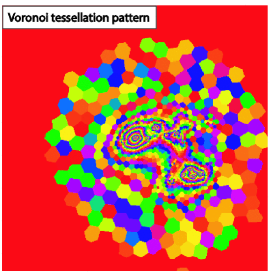
Adaptive binning provides an alternative to the smoothing approach and for this study we make use of the Voronoi tessellation code of Diehl & Statler (2006), a generalisation of the Voronoi binning algorithm of Cappellari & Copin (2003). Voronoi tessellation overcomes the drawbacks of smoothing by binning together groups of pixels to conglomerate resolution elements (frequently referred to as “spaxels”), recomputing the signal and noise in each new bin. Pixels are continuously accreted until a threshold has been met in each spaxel. The advantage of this adaptive binning method is that in high- regions, the spatial sampling remains high because spaxels are typically small, whereas in diffuse regions is improved greatly. Diffuse emission regions, by definition, show variations over much larger spatial scales. Since each individual pixel is used exactly once, surface brightness is always conserved.
The F140LP FUV science observation is assigned as the “reference” image, and used to generate the binning pattern, using the inverse variance map output by the STSDAS/MULTIDRIZZLE task to compute . Pixels are accreted into spaxels until has been met, with a maximum size of pixels ″ in order to speed up the process and prevent spaxels from growing arbitrarily large.
2.1.4 Super star clusters
Point-like sources are identified in the deepest of the optical bandpasses, F435W and F550M using the DAOFIND task in IRAF. To be considered a detection, a cluster must be present in both of these bands. Each object was then inspected by eye and any detections that were clearly spurious were removed from the catalogue. For crowded fields PSF-photometry is preferred to standard aperture methods in order to eliminate cross-contamination from neighbouring clusters. However, some clusters may be extended enough to be resolved by our observations, thus precluding the use of PSF-fitting methods and limiting us to aperture photometry. Aperture photometry was performed using the PHOT task in IRAF in all bands using the F435W+F550M detected catalogue. An aperture of 0.10″ was used, and sky was sampled in a circular annulus of radius between 0.1 and 0.15″. Aperture corrections were then applied in accordance with those given in Sirianni (2005) for the HRC and WFC bandpasses. While SBC/F140LP aperture corrections have been computed in the past, (e.g. Dieball et al., 2005), they are not available in the published literature and our own aperture corrections, computed with the TinyTim software (Krist, 1995), are included here in Table 8, Appendix A. Since we have no a priori knowledge of the continuum slope, we adopt the F140LP aperture correction for , using 0.1″ as in the other bandpasses. Since SBC/F122M contains the Ly line, no point-source photometry was performed in this bandpass itself. Instead, we perform aperture photometry on the continuum subtracted Ly and H images in the same 0.1″ apertures at the position of each cluster with no re-centering applied. This gives a direct measure of the Ly flux and equivalent width in the vicinity of each SSC.
In order to estimate the properties of the SSCs, the same SED-fitting software described in Section 2.1.2 was applied to the aperture extracted fluxes. Age, , photometric mass, etc. were computed, allowing us to compare these properties with Ly in the immediate vicinity of each SSC.
2.2 ESO – New Technology Telescope
Haro 11 was observed during the nights of 18, 19, and 20 September 2004, using the New Technology Telescope at ESO La Silla, as part of an observing run to obtain H, H, and [Oiii] narrowband images for all southern targets in our HST Ly sample (Atek et al., in preparation). On the night beginning 18 Sept seeing was good, not exceeding 1.2″for the duration, although thin cirrus prevents a direct calibration of these data. On the night of 19 Sept, observational conditions were ideal: photometric and with sub-arcsecond seeing throughout. The final night was still photometric but seeing deteriorated to ″ and images were unusable for science purposes. The good-seeing data from the night of 18 was calibrated through secondary standard stars in the field, using data from the photometric nights of 19 and 20 Sept. Narrowband imaging was performed at H, H, and nearby continuum. Spectrophotometric standard stars LDS749B, Feige 110, and GD50 were selected (on the grounds of their high spectral resolution: Å, in order to resolve the stellar absorption features around H and H) from the catalog of Oke (1990), and were observed at regular intervals for the duration of each night in all filters. Imaging observations were performed using both the ESO Multi-Mode Instrument (EMMI) (Dekker et al., 1986) and Super Seeing Imager 2 (SuSI2) (D’Odorico et al., 1998), interchangeably. The instruments were used in pixel binning mode to reduce the readout noise, providing a plate-scale of 0.1665″ pix-1 and 0.130″ pix-1, and a field-of-view (FoV) of ″ and ″, for EMMI-R and SuSI2, respectively. Table 2 summarises the imaging observations included in this article, lists the ESO filters used, and the total exposure times in each band.
| Observation | Camera | ESO filter # | ExpTime [ s ] |
|---|---|---|---|
| H | EMMI-R | 598 | 900 |
| H cont. | EMMI-R | 597 | 1200 |
| H | SuSI2 | 549 | 2866 |
| H cont. | EMMI-R | 770 | 1800 |
Data were first reduced by the standard routines in NOAO/IRAF: bias subtraction and flat-field correction using well exposed sky- and dome-flats. Images were aligned using the GEOMAP/GEOTRAN tasks and smoothed to the seeing of the worst seeing image using the GAUSS task. All HST bandpasses are aligned with the NTT frames and the PSF is degraded by convolution with a Gaussian kernel. H and H were continuum subtracted to obtain the nebular emission fluxes, accounting for contamination by [Nii] (H only) and underlying stellar absorption. [Nii] contamination is estimated using [Nii]Å/H (Bergvall & Östlin, 2002). Stellar absorption is estimated from the best-fitting Starburst99 spectrum at each pixel by modifying the spectral fitting code described in Sect. 2.1.2. The Starburst99 stellar libraries (Martins et al., 2005) were built upon the latest model atmospheres and include full line-blanketing for all stars and non-LTE effects for hot stars, thereby providing the best estimate of the stellar absorption features available. With the age of the stellar population we measure the equivalent width of H using the same line and continuum wavelength windows as the Lick index (Worthey et al., 1994). The windows used for H are of the same size as those for H, but scaled to H (i.e. the same windows ). is generated from H/H, assuming a temperature of 10,000 K and intrinsic line ratio of 2.86, using the extinction law of the SMC following Gordon et al. (2003); Fitzpatrick & Massa (1988).
2.3 X-Ray: Chandra and XMM-Newton
Haro 11 happens to be located 14′ away from the Cartwheel galaxy, of which X-ray observations have been obtained with both the Chandra and XMM-Newton telescopes (Wolter & Trinchieri, 2004). Respective total integration times in Chandra and XMM-Newton were 80 and 70 ksec. Regarding XMM-Newton, Haro 11 only falls within the field–of–view of the MOS2 detector, having unfortunately been missed by both the MOS1 and PN chips. Both the Chandra and XMM-Newton datasets have been obtained from their respective archives. Since both telescopes operate with curved focal-plane configuration, the point spread function degrades severely with angular distance from the optical axis. For the XMM-Newton detection, the PSF is so distorted that all spatial information has been lost, but the object is bright enough that a one-dimensional spectrum can be extracted from the MOS2 data. In the Chandra observation, Haro 11 lies on the S1 chip: the object is clearly detected and we were able to perform a spatial analysis of the source (see Sect. 3.2).
The Chandra data were processed following the X-Ray Data Centre pipeline software. The level 1 events were reprocessed using Ciao 3.4 task acis_process_events. The whole band (0.2-10 keV) image was smoothed applying the csmooth task. The image was smoothed with a minimal signal–to–noise of 3 using a circular Gaussian kernel. The source spectrum was extracted from a circular region of radius 30″. The background was obtained from the combination of four circular regions located close to the source and avoiding other X-ray sources in the field. Source counts were grouped to have at least 20 counts per bin to allow modified minimisation technique (Kendall & Stuart, 1973) in the spectral analysis. Redistribution matrix and auxiliary response matrix files were generated.
The XMM-Newton data were processed using the standard Science Analysis System, SAS, v.7.0.0 (Gabriel et al., 2004). The most up-to-date files available as of January 2007 were used for the reduction process. The time intervals corresponding to high background events were removed using the method followed in Piconcelli et al. (2004). The resulting exposure for the MOS2 data is only of 44 ks. No sign of pile-up was found in the MOS2 image, according to the epaplot SAS task. A visual inspection of the 0.2-10 keV image shows a distorted shape due to location of the source, close to the edge of the CCD. Therefore, no further analysis of the XMM-Newton image has been performed. The source spectrum was obtained, as for the Chandra observation, from a circular region with a radius of 30″. The background was extracted from a circular region close to the source and avoiding other X-ray sources in the field. Source counts were grouped to have at least 20 counts per bin. SAS appropriate tasks were used to generate the distribution matrix and auxiliary response matrix files.
On-axis observations of Haro 11 have also been obtained with the Chandra telescope (Grimes et al., 2007) although their archive status is still proprietary. Quantities derived from that dataset are, however, compatible with those presented here using off-axis archival observations (see Section 3.2).
3 Results
3.1 Lyman-alpha, UV and optical
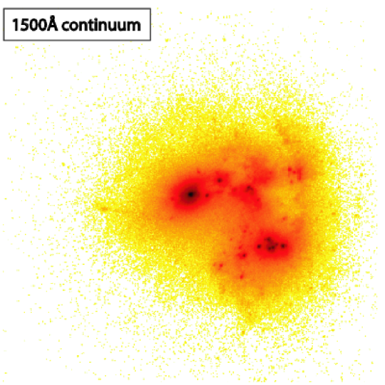
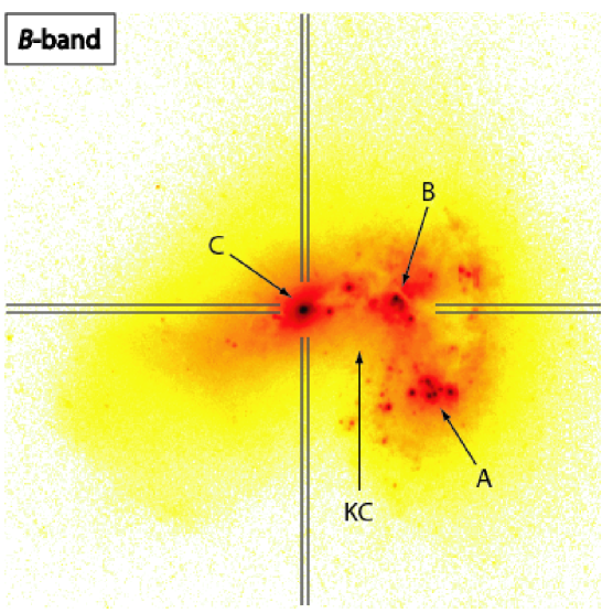
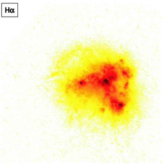
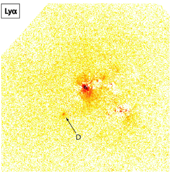
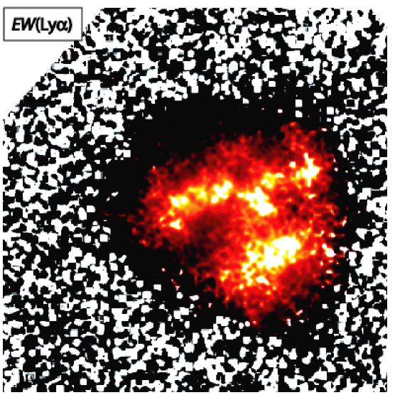
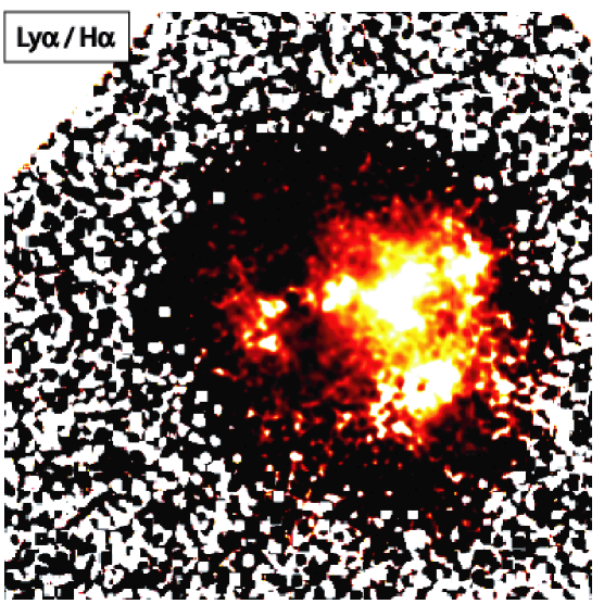
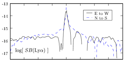
Figure 1 shows the results of the processed HST observations. This panel of figures shows Haro 11 in FUV continuum and band, continuum subtracted Ly and H, , and Ly/H. An inverted log-scale is used showing emission in yellow to black. Significant star-forming condensations (Kunth et al., 2003) and the approximate kinematic centre (Östlin et al., 1999) are marked in the band image. Other maps show the position of the SSCs and the Voronoi tessellation pattern. Plots at the bottom of the figure show the spatial variation of Ly, , and Ly/H along horizontal and vertical lines through the brightest Ly point, the positions of which are marked in the band image.
We note that H emission loosely follows that of the FUV continuum (as would be expected from star-formation signatures) although there are a few differences. Notably, the brightest H knot () is not the brightest UV source (knot ). This could be an effect of age, dust, the density of the surrounding gas, or a combination of all three. The Ly images on the other hand, resemble neither the UV nor H. Knot shows strong central Ly emission with two other patches of more diffuse emission to the north-west. Absorption is seen throughout the region of knot and emission and absorption can be seen varying on small (pc scales) around knot , although overall the absorption dominates. A compact, isolated emission source to the south-east appears in the continuum subtracted image and is labeled knot . More generally, however, the Ly emission appears in two distinct components: a central bright region and a surrounding diffuse, largely featureless, halo component. In the following analysis we identify these as the central and halo emission regions as two different physical components.
Haro 11 has been observed through the low-resolution Short Wavelength Prime (SWP), ″ elliptical aperture of the IUE satellite. We obtained the IUE spectrum from the archive and have measured the IUE Ly flux to be erg s-1 cm-2 with an equivalent width of 14.8Å. Photometry of our Ly image in an aperture designed to match that of the IUE reveals a flux of erg s-1 cm-2 and equivalent width of 14.3Å. This flux is fully consistent with the photometric error on the IUE measurement of around 10%.
Kunth et al. (1998) presented Ly measurements obtained with the GHRS. This spectrum was obtained after a sequence of small angular maneuvers (SAMs), designed to find the peak in FUV surface brightness. Information about the SAMs is not available and the FUV morphology is so complex that it is not possible to reconstruct the maneuvers made by the telescope. In a ″ aperture centred on , the continuum flux measured in the ACS frames is a factor of 4 brighter than that in GHRS, and apertures centred directly upon and both show Ly in absorption. We are unfortunately not able to test our ACS fluxes against this observation, despite numerous efforts to predict the PEAK-UP behaviour: it’s most likely the telescope centred somewhere between the three knots.
The total emergent Ly line-flux measured in the image is erg s-1 cm-2, corresponding to a luminosity of erg s-1 for our assumed cosmology.
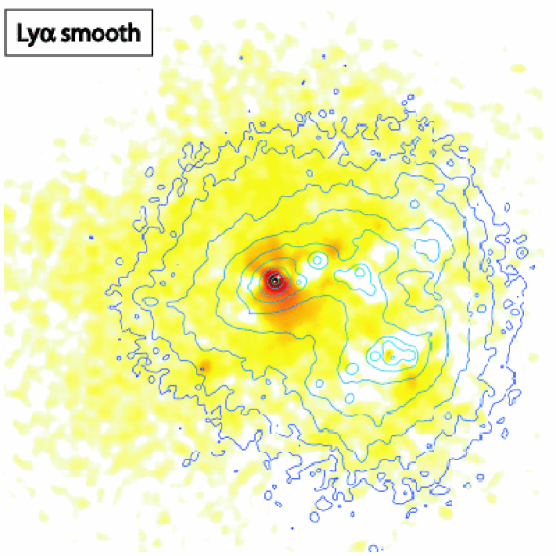
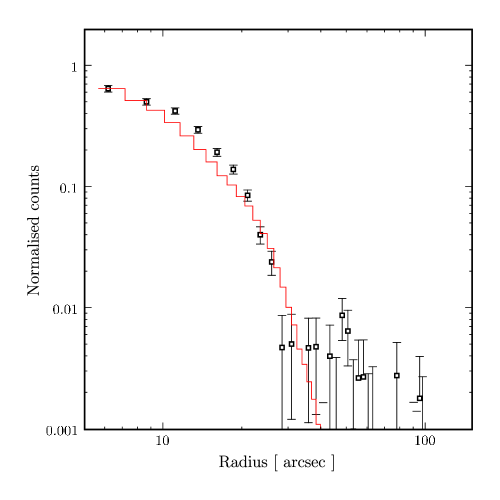
To eye the Ly image is so azimuthally symmetric that we deem it informative to present a radial surface brightness profile of continuum-subtracted Ly, shown in Figure 2. This was generated by integrating the flux in concentric annuli of width 2 pixels, centred on the brightest central pixel of knot . The central and halo components identified in the Ly map are clearly visible in the surface brightness profile, with the central component taking over at around 0.5″. Since they are so clearly independent (visually resembling a bulge+disc morphology) we fit Sérsic functions to the halo and central excess (i.e. total–halo) components using the formula
| (1) |
where is the central surface brightness, is the effective scale length, the Sérsic index. Integration from zero to infinity then gives back the total flux in each component. The results of the profile fitting in the two components can be seen in Table 3. The regions chosen for fitting in the two components were 0-0.5″ and 1-7″for the central region and halo, respectively.
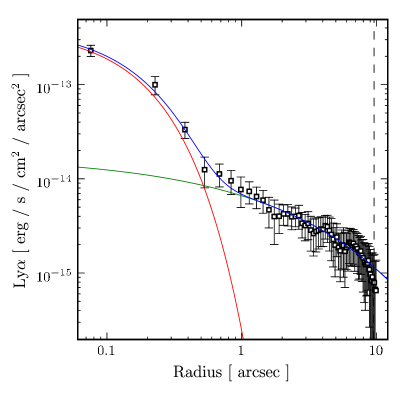
| Component | [ ″ ] | ||||
|---|---|---|---|---|---|
| Halo | 2.12 | 1.05 | 2.2 | 76.4 | 6.93 |
| Central excess | 47.8 | 0.134 | 1.0 | 5.64 | 0.512 |
| Total | – | – | – | 82.0 | 7.44 |
| Measured total | – | – | – | 79.6 | 7.22 |
We have also Voronoi binned the individual images. Since Voronoi binning conserves surface brightness across each spaxel, we can directly compare Ly surface brightness with other fluxes or properties without a loss of reliability in lower surface brightness regions. With binned images in hand, we present the Ly surface brightness and Ly/H as a function of various other parameters in Figure 3.

Each point represents the surface brightness in each resolution element, although the elements themselves vary from single pixels to 1600-pixel (1 ″) spaxels. Also, since fluxes are presented on log-space, only resolution elements that are positive in Ly are shown, eliminating regions of absorption. It is not possible to estimate global or integrated values from these scatter-plots; histograms of the distributions are presented above and to the side of each scatter plot, in order to better give a feeling for this. The left-most two plots show how the Ly emission and line ratio correlate with H and the age of the young stellar population. The Ly vs. H plot is again suggestive of two distinct pixel components. One at lower H surface brightness (erg s-1 cm-2 arcsec-2) in which Ly appears largely independent of H. This feature extends over approximately three orders of magnitude in H and the Ly/H plot shows the emission is always above the value that would be expected from recombination theory. Above the quoted H surface brightness, the distribution changes and an upper limit appears to be set by the recombination value. The line ratio plot clearly shows that Ly photons are emitted from regions where the H flux would suggest that little nebular gas is present. A similar effect is also seen in the second plot where Ly is compared with the age of the stellar population and there is evidence for substantial amount of pixels showing Ly emission with ages in excess of 100 Myr; much too old to produce nebular emission. The right-most two plots show how Ly correlates with the as determined from fitting the stellar UV continuum (), and continuum slope itself (). Since in part reflects , these two plots correlate somewhat in shape, although is also dependent upon age. The discrete values of from the fitting grid are apparent. Again the distribution signifies a non-continuous distribution of pixels: in both cases Ly can be seen in emission from regions with extending up to 1, and showing a very red slope. In these regions of the plots, emission is again found almost exclusively above the recombination value. At lower () and () the pixel distribution changes and broadens significantly in both Ly and Ly/H. The Ly surface brightness tends to increase in these regions although the bulk of the pixels show line ratios significantly below the recombination value. While brighter overall, these emission regions show strong attenuation of Ly.
Figure 4 shows how correlates with gas-phase interstellar extinction, , as determined from the Balmer decrement and is partly similar to the right-most plots in Figure 3.
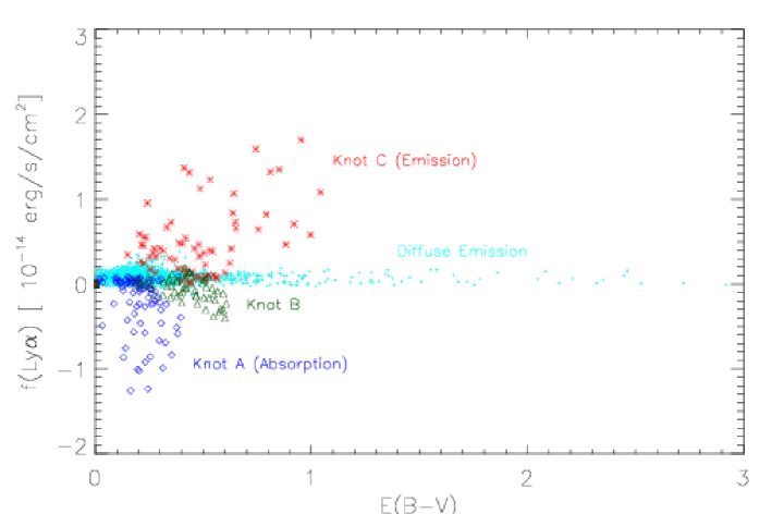
This provides a much less biased estimate of dust extinction compared to the approximation obtained by spectral modeling of the stellar continuum. Table 4 shows the values of obtained by measuring H and H in 1″ circular apertures centred on knots , , and , together with the values obtained spectroscopically by Vader et al. (1993). With the spatial sampling in HST images degraded by two orders of magnitude to match the ground-based seeing, we cannot resolve the fine details of the Ly emission and the surface brightness range is significantly reduced. is here presented in linear space and now shows regions of absorption, most notably around knot . This distribution shows a structure partially resembling that of the Ly vs. plot: a component of diffuse, low surface brightness Ly emission is seen extending beyond , with a brighter Ly emission region (knot ) where shows a large spread, with a mean value of 0.48.
| NTT H/H | 0.20 | 0.42 | 0.48 |
|---|---|---|---|
| Vader et al. (1993) | 0.16 | 0.41 | 0.39 |
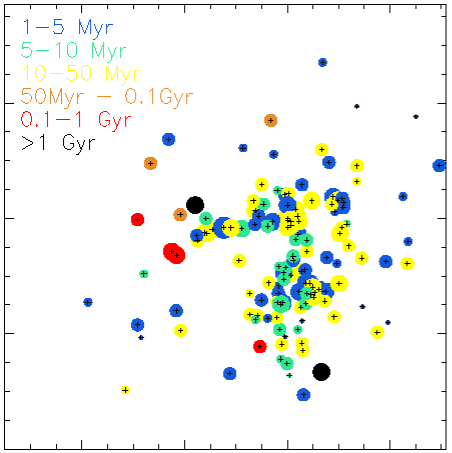
In total we find 140 star-clusters. The spatial distribution, together with the ages and masses of these clusters can be seen in the upper-right panel of Figure 1. The age and mass distribution of the clusters can be seen in Figure 5.
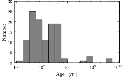
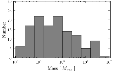
The decrease in the mass distribution at is the result of incompleteness in the less luminous clusters. While there is much of interest in these data, most of it is outside the scope of this article and will be presented in a forthcoming publication (Adamo et al., 2007 in prep); here we simply deal with the relation between a few basic properties and Ly.
3.2 X-ray: XMM and Chandra
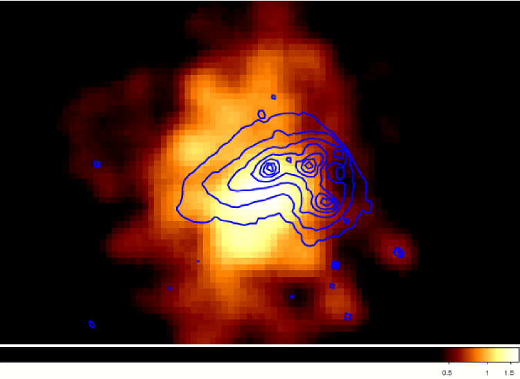
In the upper panel of Figure 6 we show the Chandra image of the full energy range (0.3–8 keV) adaptively smoothed (see Sect. 2.3). Continuum contours from the ACS/F140LP observation have been overlaid to show the location of the different knots. The lower panel in Figure 6 shows the X-ray surface brightness profile, in the 0.2–2 keV range compared with the corresponding profile of the off-axis PSF of ACIS-S1 at 1.5 keV. The plot shows hints of extended emission visible in the 20–40 px region, i.e. 10-20 ″ (1 pix = 0.492″). The Chandra image shows a central unresolved core region and a weak, diffuse hot gas component, emitting over an area ″ in diameter. The diffuse component appears more extended in the north-–south direction than in east–-west. However, no firm conclusion can be reached as the image is largely distorted due to the ′ offset from the Chandra nominal on-axis location. In fact, the Chandra on-axis images of Haro 11 reported by Grimes et al. (2007), shows different emission knots following the optical/UV emission structure. The brightest peak of the Grimes et al. (2007) image coincides with knot , while the maximum emission on our image is located closer to knot and more than 5″ from knot . A plausible explanation for the observed mismatch could be variability, although the spectral analysis, fluxes, and luminosities of both observations are in good agreement (see below). Therefore, the more likely explanation could be the intrinsic Chandra astrometry uncertainty, although we note that this is only of the order of 2″ for off-axis observations.
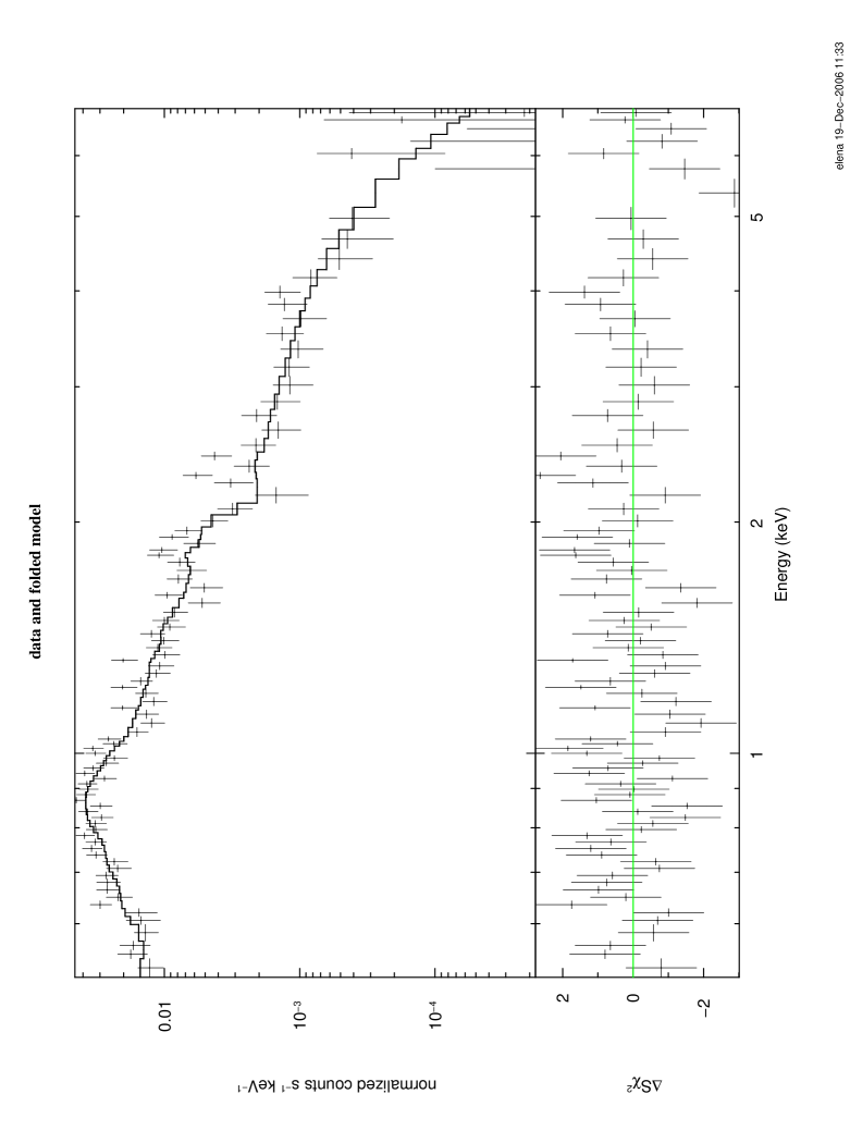
Spectral analysis was performed on both Chandra and XMM-Newton data, in order to derive the spectral shape of the source, the X-ray luminosities and, local photoelectric absorption column density of Hi. The observed spectrum was corrected for Galactic absorption, cm-2 (Kalberla et al., 2005; Bajaja et al., 2005). The Haro 11 spectral emission is complex: both power law and thermal single–component emission models provide unsatisfactory fits to the data, with values equal to 2.2 and 3.5, respectively. The best-fit model consists of a combination of a power-law and mekal model (Mewe et al., 1986). Statistically indistinguishable results were obtained applying a double thermal mekal model. However, the temperature of the hottest thermal model is keV. This high value is difficult to explain in a standard physical scenario. We have also derived an upper limit for the absorption equivalent Hydrogen column of cm-2. Figure 7 shows the X-ray spectrum together with the best fit model and the corresponding residuals. The values of the parameters and the goodness of the fit are listed in Table LABEL:tab:xraypars. The corresponding total X-ray fluxes and unabsorbed luminosities are shown in Table LABEL:tab:xrayflux. Even though the effective area of XMM-Newton is larger than that of the Chandra, the MOS2 spectrum of Haro 11 resulted in lower signal–to–noise. This is mainly due to the short real exposure time (44 ks) after the high background filtering, combined with the fact that the source is only visible in MOS2, for which the effective area is 3 times lower than that of PN. However, the source MOS spectra was analysed, confirming the results obtained with Chandra. A single–component model (power-law or thermal emission) failed to reproduced the data. The best fit model consists also of a power-law with and a mekal component with . All the parameters derived from the XMM-Newton spectrum are compatible within the error with those from the Chandra analysis. We have measured a somewhat lower value of the high energy flux, of the order of 65%. The quantities derived from our spectral analysis are compatible with those derived from on-axis Chandra observations presented in Grimes et al. (2007).
| Parameter | Value | Unit |
|---|---|---|
| Intrinsic | cm-2 | |
| Power-law photon index | ||
| Mekal kT | keV |
| Band [ keV ] | Flux | Luminosity |
|---|---|---|
| 0.5 to 2 | ||
| 2 to 10 | ||
| Total |
4 Analysis and discussion
4.1 Lyman-alpha morphology
Figure 1 shows some of the imaging results. Visual inspection clearly reveals that Ly morphology is not representative of either H or the FUV continuum. The overall Ly morphology exhibits a central bright emission source (centred on knot ), with a diffuse, largely symmetric halo-like component with lower surface brightness. The emission around is more extended in the north–south directions compared to east–west, and appears as two fan-like structures of size ″. This structure is not seen in maps and may be due to a filamentary Hi structure. Typically and Ly/H are low in the central regions, where continuum and H are strong, but increase dramatically in the outer regions. Some absorption spots are seen in the regions around knots and . The most likely interpretation of this overall morphology is that photons are escaping directly from the central regions, either through winds or ionised holes in the ISM, while the halo component arises from resonance scattering of Ly.
Knot , the small blob of Ly emission found in the analysis of (Kunth et al., 2003) is clearly visible towards the south–west. Knot is not visible in any of the continuum bands or the H on-line observation and it appears to be a real source of Ly photons devoid of continuum.
The radial surface brightness profile presented in Figure 2 shows the flux in the halo component decaying approximately exponentially with radius, but peaking sharply in the centre. The fan-like structures described above are contained within the central surface brightness peak. Fitting Sérsic functions to these two independent components and integrating under the best-fitting formulae allows us to measure the relative contribution of the components of central and halo emission, and shows that while surface brightnesses are significantly lower, % of the photons are emitted via the photon diffusion mechanism. This is comparable to the value of % in the halo component of ESO 338-IG04 presented in Hayes et al. (2005), although for that study the estimate was made by masking the images instead of profile fitting. The two galaxies are comparable in FUV luminosity, both low-metallicity, and both exhibit complex dynamical and morphological structures, and the Ly output of both are clearly dominated by the halo mechanism.
4.2 Lyman-alpha production, escape and regulation
In the H image we measure a total line flux of erg s-1 cm-2, identical to that given in Schmitt et al. (2006), which is not corrected for Galactic extinction. Galactic extinction correction (Cardelli et al., 1989) gives a intrinsic H flux of erg s-1 cm-2, consistent with Östlin et al. (1999). The total Ly production estimated from the case B recombination gives a value of erg s-1 cm-2. Adopting the Ly flux we obtained by integrating the (Galactic-extinction corrected) surface brightness profile we obtain a Ly escape fraction of just 2.7%. This calculation neglects the fact that Ly can be enhanced relative to H by shock excitation. Were there a significant contribution to Ly as a result of a shocked ISM, this escape fraction will be further reduced.
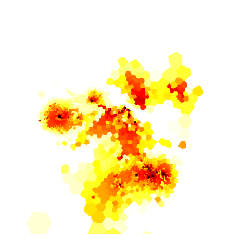
Plots of the Ly surface brightness in each binned element, compared with various other quantities, are seen in Figure 3. Most importantly, these plots show how the Ly surface brightness spatially compares with H and the dust distribution. The left-most plot shows Ly vs. H; the red lines indicate Ly=H line and Ly/H=8.7 (case B recombination). Comparing Ly to H also identifies two independent components of Ly emission. Firstly, at low Ly and H surface brightness ( and erg s-1 cm-2 arcsec-2 for Ly and H, respectively), the Ly to H ratio seems to always exceed that predicted by recombination (see Ly/H spatial distribution in Figure 1). Again, shock excitation could enhance the production of Ly relative to H, and it’s plausible that some of the Ly is produced in a shocked ISM. Indeed, this is an oft-proposed mechanism for Ly production in high- Ly-blobs (LABs), resulting in large-scale Ly emission with little or no associated continuum. However, without observations in other emission lines the exact mechanisms at play in LABs are very difficult to test, although tests may be performed for targets at low- observed with HST. Optical spectroscopy of Haro 11 performed by Heisler & Vader (1994) and Kewley et al. (2001) consistently find spectra consistent with pure photoionisation nebulae. On the other hand, these spectra were extracted in large apertures centred on the knots, avoiding diffuse Ly emission regions, and the answer is not fully conclusive. It is possible that future high resolution spectroscopy (e.g. with a repaired STIS) may be able to test this directly. Given the resonant nature of Ly a more likely interpretation of this Ly–H decoupling is that it arises from resonant scattering of Ly photons. The Ly/H histogram in Figure 3 confirms that over 50% of the pixels are in the component with super-case B line ratios. The fact that these points are here most likely indicates that a significant number of Ly photons must have travelled far from their point of origin, undergoing numerous resonance scatterings.
At higher surface brightnesses ( erg s-1 cm-2 arcsec-2 for H), the distribution clearly changes. Here the recombination value seems to set an upper limit on the Ly/H ratio and Ly is never stronger than expected. The top edge of this distribution must result from Ly photons escaping the galaxy directly either due to ionised holes in the ISM cleared by the UV radiation field or through a rapidly outflowing neutral medium. The distribution fans out in this component and a large spread in Ly surface brightness is seen which results from either resonance scattering selectively removing Ly photons from the line-of-sight (from where they may be re-scattered and emitted in the halo component) or destruction by dust. The central emission region also shows absorption structures to the east and west of knot (see middle-right panel of Figure 1), where this effect may be strongest.
The resonant decoupling of Ly photons is also revealed in Figures 3 and 4, where Ly is compared with from fitting to the stellar continuum (), H/H (), and . If Ly were a non-resonant line a declining relationship would be expected between Ly and . The bulk of the Ly output is in the halo component (Ly surface brightness erg s-1 cm-2 arcsec-2; Figures 2 and 3). Below this level, there is essentially no trend of Ly with . Most importantly, when Ly is seen in emission from regions with it is almost entirely with line ratios that exceed the recombination value. This uncorrelated faint emission component is also seen in the plot where the distribution of diffuse pixels (shown in cyan) is constant over the whole range of . Despite the low dust content of knot (mean ), Ly is seen only in absorption in this region. In contrast, the brightest Ly region (knot ) shows Ly only in emission with measured values of as high as 1, although the regions , & have sizes comparable to the seeing disc in the ground-based images and therefore the scatter at each knot may be an artefact (the mean value of in knot is 0.48). Ly reaches its brightest flux levels where is small which is symptomatic of the contrasting escape mechanisms, but it must be noted that this only accounts for around 10% of the overall Ly output. That we see such strong absorption from knot but emission from knot seems to indicate that the static Hi column density in the line-of-sight to knot must be significantly greater than to knot . Knot does contain several massive clusters, the ages of which are consistent with the high mechanical luminosity (Leitherer et al., 1999) that would be required to drive out the neutral ISM, although it seems that either the Hi covering is too great, or the clusters are too young to have accelerated the surrounding medium. Unfortunately we have no direct information on the Hi column density or the mechanical energy return that would be required to drive a superwind.
That we see Ly from resolved regions with is a striking result. For a simple dust slab this would correspond to the loss of more than 99.9% of Ly photons, before scattering is considered. Since in the halo regions we typically see Ly/H above the recombination value we can infer that radiative transfer effects are at play in the propagation of Ly photons, and scattering events have caused these photons to travel significantly increased path-lengths. Again, knowledge of the geometry and kinematics of the neutral and ionised media would be required to infer the number of scatterings, mean free paths, and therefore the actual path-lengths involved. We can, however, identify two possible extremes of the photon transport mechanism. Firstly, they may have diffused through largely static Hi gas with transport dominated by multiple rare scatterings into the wings of the distribution function. In this case, the neutral medium must be pristine, dust-free, and have never mixed with star-forming regions. Secondly, and much more likely, much of the propagation may have been through paths in the low-density ionised ISM with scattering/reflection events occurring at the surfaces of dense neutral clouds. In the multiphase ISM models of Neufeld (1991) and Hansen & Oh (2006), such a geometry shields Ly from the dust that is embedded in the Hi, with reflections preserving Ly by preferential propagation in the ionised ISM. Transport effects in these models suggest that equivalent widths may be significantly boosted, even globally. The global Ly equivalent width and line-ratio are certainly not boosted, and what we are seeing may be preferential Ly destruction in some regions and relatively unhindered transport in others. Where the bulk of the Ly destruction is taking place, we cannot say. Either way, the transport effects result in the superposition of Ly photons on top of dusty and/or old stellar populations.
A two dimensional kinematic study of Haro 11 has been performed in the H line by Östlin et al. (1999, 2001) using the CIGALE Fabry-Perot (FP) interferometer on ESO’s 3.6m telescope. These data demonstrated the kinematic centre to lie approximately midway between knots and as labeled in Figure 1, with the major axis lying in the NW-SE direction with the NE side toward knot receding. In the central 2″(1kpc) iso-velocity contours are shown to be densely packed and show a steep rise in rotational velocity in the direction of knot , indicating a non-relaxed system or possible second kinematic component. While we expect even the diffuse Ly emission to be in part regulated by the kinematic structure of the ISM, we are not able to see any correlation between Ly and velocity shifts or shear in the ISM. The resolution of the CIGALE data is not sufficient for us to compare small-scale Ly emission/absorption features with the kinematic structure of the ISM, although on larger (kpc) scales no correlation is apparent. Moreover, turbulence or disruptions in the ionised medium does not necessarily imply the neutral ISM has been accelerated.
In summary we see clear evidence that, while Ly photons must be produced in the same regions as H, we do not observe them to be emitted from their production sites, and the bulk of the Ly photons travel significantly enhanced path lengths. We see no relationship that would indicate Ly correlates spatially with the dust distribution. Unfortunately we do not have information about the Hi distribution or its kinematic structure.
4.3 Lyman-alpha and the SSC population
The age distribution of the super star cluster population are shown in Figure 5. Figure 8 shows the equivalent width of Ly in the immediate 0.1″ of the super star clusters, compared with the respective age of each cluster. Ly equivalent widths are measured from the continuum-subtracted and continuum-only image in fixed apertures.
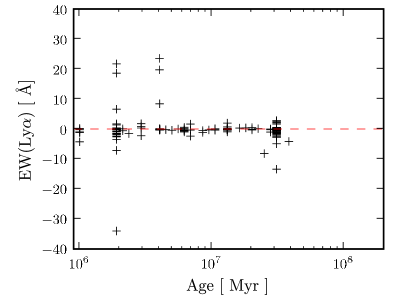
Tenorio-Tagle et al. (1999) and Mas-Hesse et al. (2003) have presented evolutionary studies of Ly emission from starbursts which qualitatively predict the evolution of with age. The Ly sequence is more complex than that of H due to the resonant trapping of Ly photons in Hi resulting in a need for mechanical feedback and/or a higher ionisation fraction to create a medium optically thin to Ly. The model is such that at very young ages ( Myr) the Ly feature is expected in absorption due to dense, static Hi medium. After some time, the cluster is able to ionise this medium and drive out an expanding shell resulting in a pure emission feature between 2.5 and 5 Myr. As the expanding shell recombines, the Ly emission feature develops a P Cygni-like profile which, with continuing recombination removes successively more of the emission until, at around 8 Myr, the Ly feature is again in absorption. With such a large number of SSCs (effectively mini galaxies) and Ly maps, this evolutionary sequence becomes something we could possibly examine within our dataset. However, there are a number of factors which could mask such a relationship, particularly in a dataset consisting of imaging observations only. Firstly, when the feature is P Cygni some or all of the emitted flux is cancelled by the absorption profile, resulting in termination of the observed Ly emission phase at earlier times than predicted. Secondly, geometry also enters into the model and, due to the ionisation structure being cone-like, the orientation must be favourable in order to observe the Ly emission phase. In our dataset, this will result in a decrease of or complete absence of Ly from some Ly emitting clusters. Thirdly, due to the diffuse emission, Ly can be seen from essentially any region of the galaxy. However, due to the high continuum levels around SSCs, strong contamination is not expected and will also be accounted for by background subtraction. Finally, a general spread can be expected due to variations in the initial cluster mass, Hi distribution, mechanical feedback requirements, and internal absorption that is not local to the cluster itself. What we could possibly expect is negative at the earliest times, becoming positive and peaking between 2.5 and 4 Myr, and then declining again to the background levels at around 6 to 8 Myr. Spread is expected toward lower (and negative) due to orientation effects and the Hi covering. Moreover, the noisy nature of the continuum-subtracted Ly map further complicates very local equivalent width measurements. We consider only the sub-population of clusters with age below 40 Myr. Figure 8 does show a distribution of peak vs. age that is quantitatively consistent with the evolutionary models. For the lowest ages Ly is seen only in absorption or around the zero-level. For ages between 2 and 4 Myr some SSCs show local Ly emission that could possibly represent the emission phase, although there is some spread. At late times ( Myr) Ly is only seen in absorption or very close to zero.
4.4 X-ray information and star formation rates
The Chandra image (Figure 6) shows that most of the X-ray photons have been emitted in a region surrounding knot . The radial profile of X-ray emission is largely featureless. Comparing the radial profile with the Chandra off-axis PSF (Figure 6) yields some hints of extended emission up to around 10–20″. The X-ray emission arises from the same region around knot where Ly is brightest, suggesting that Ly emission from this region might be the result of a perturbed and outflowing ISM, accelerated by the release of mechanical energy from the SSCs located at knot . However, it is worth noting that the analysis of an on-axis Chandra observation of Haro 11 (Grimes et al., 2007) indicates that the emission is resolved in several knots, the brightest one coinciding with knot .
We have measured an upper limit for the equivalent Hydrogen absorption column of cm-2. We want to stress that consistent fits could also be found with lower columns: the F-test gives only a probability around 90% for the fits using this value of the column density, so that the present data do not allow us to constrain the amount of neutral Hydrogen in front of knot . In any case, column densities around cm-2 were obtained by Kunth et al. (1998) from Voigt profile fitting of the Ly absorption profile in the GHRS spectrum ( cm-2), and Verhamme et al. (2006) note that Voigt profile fitting may systematically underestimate . It is interesting to note that Haro 11 showed the largest Hi column density in the 4 galaxies of Kunth et al. (1998) with Ly emission ( cm-2). The derived temperature of the hot diffuse component is K, a typical value also found for other local dwarf-starbursts like He 2-10 and NGC 4449 (Grimes et al., 2005).
| Tracer | SFR | Source | Calibration reference |
|---|---|---|---|
| 1.4 GHz | 5.6 | VLA | Condon (1992) |
| FIR | 18 | IRAS | Rosa-González et al. (2002) |
| H | 24 | HST | Kennicutt (1998) |
| 1527Å | 19 | HST | Rosa-González et al. (2002) |
| 0.5-2 keV | 22.0 | Chandra | Ranalli et al. (2003) |
| 2-10 keV | 26 | Chandra | Ranalli et al. (2003) |
In Table LABEL:tab:sfr we present star-formation rates (SFR) derived from X-rays, other observations in this study, and previous observations from the literature. Within the errors, star formation rates derived from FUV continuum, Far Infrared (IRAS FIR, corrected to the 1–1000 range according to Helou et al. (1988)), H and X-ray luminosities are consistent with a SFR M⊙ yr-1. Such a SFR is rather high and could explain the presence of high-velocity winds and disrupted interstellar medium, driving the Ly escape and pushing hot and neutral gas to a large radial extent. Compared to the sample of Ly emitters at from Gronwall et al. (2007), Haro 11 appears at the top end of the SFR distribution they derive from the FUV continuum (within the range 1–40, with an average value around 5 M⊙ yr-1). This implies that Haro 11 is a very actively star-forming galaxy in the local Universe, comparable to the objects being analysed at high redshifts and the results obtained from its analysis may therefore be directly applicable to more primeval systems.
The fact that the SFRs derived from the X-ray emission are pretty consistent with the values derived from FUV continuum, H and FIR emission implies that the X-ray emission should be driven by the powerful star formation processes taking place in Haro 11, with no hint on the presence of a low luminosity active nucleus at the core of knot . Indeed, the ratio of is very close to the average value found by Ranalli et al. (2003) for a sample of star-forming galaxies at redshifts in the range 0.2–1.3. A preliminary analysis based on the models of Oti & Mas-Hesse (2007, in prep) shows that this ratio is consistent with a powerful star formation process dominated by SSCs with age below 5 Myr, with a standard efficiency of around 10% in the transformation of released mechanical energy into thermal X-ray emission.
On the other hand, the radio luminosity yields a significantly lower value of the star formation rate when compared to the other tracers. We believe this is due to the youth of the star formation episodes in Haro 11. The calibration used assumes a steady star-formation process with radio contributions from both thermal and non-thermal components (synchrotron emission from supernova remnants). Figure 5 shows that most of the SSCs are younger than around 3.5 Myr, so that the number of supernovae expected from the slightly older SSCs is significantly smaller. The low radio emission could therefore be explained by this deficit in the non-thermal component.
The relative hardness of the X-ray continuum (photon index ), indicates that the hard band, contributing % of the X-ray output, might be dominated by high-mass X-ray binaries (HMXB). Since HMXBs become active after 3-4 Myr of evolution, we believe that these sources could be already present in the SSCs with age between 4 and 10 Myr. Indeed, an SSC of mass with an age of 8.2 Myr identified near knot could be already hosting a significant number of HMXB. The observational properties are therefore consistent with the distribution of ages shown in Figure 5: old enough to have produced the number of HMXBs seen in the hard X-ray bands, but still young enough not to have generated so many SNe that the radio luminosity would be dominated by synchrotron emission.
4.5 Lyman continuum production and emission
FUSE observations (Bergvall et al., 2006) have shown Haro 11 to be an emitter of LyC radiation, with an observed flux density at 900Å (,e) in the 30″30″ aperture of erg s-1 cm-2 Å-1. Subsequent re-analysis of the data (Grimes et al., 2007) place ,e at a lower value of erg s-1 cm-2 Å-1 although the answer is not yet conclusive. Bergvall et al. (2006) estimated the intrinsic LyC production by summing the measured LyC leakage and an estimate of the ionising flux computed from H and recombination theory. This translated to an escape fraction of between 4 and 10% assuming a Salpeter IMF, although the higher value is reduced to % in the analysis of Grimes et al. (2007). However, this method of estimating ,0 is difficult to calibrate for a given wavelength since Hi is ionised by all photons with Å, not just those at 900Å.
As described in Section 2.1.2, our software also outputs maps of the intrinsic , based upon the normalisation of best-fitting population synthesis models. This relies upon stellar continuum and allows us to predict directly the value of ,0 at each pixel, thereby giving a different, and possibly more robust handle on the ionising photon budget than that estimates based upon H alone: H estimates provide and upper limit on the stellar ionisation budget since shock excitation of H is neglected, while stellar continuum fitting cannot account for ionising photons that arise from non-thermal processes. However, in light of the tight correlation between between X-ray determined SFR and SFRs determined by other methods, we do not expect a significant non-thermal contribution.
Figure 9 shows a map of the ionising photon production, zoomed in on the central star-forming regions (i.e. the sites of LyC production). As expected, the LyC morphology itself resembles that of H, with knots , , and showing up as strong production sites. Knot is the brightest of the three in LyC, consistent with indications from the H that it is the most intensely ionising source. An apparent dust lane is seen north–west of which is seen in the FUV continuum and optical bands, and may represent the failure of the implementation of ‘dust screen’ extinction laws to recover all the intrinsic 900Å flux when dust is distributed along the line–of–sight. Since the method of computing relies on the normalisation of model spectra, can never be negative and pixel-to-pixel noise can introduce a spurious positive contribution to the integrated flux. Here we deal only with the Voronoi-binned images in order to better control the background noise.
Summing the 900Å flux we obtain a total value of erg s-1 cm-2 Å-1. This translates into a 900Å escape fraction, , of 9%. This is towards the upper end of the range presented in Bergvall et al. (2006) but, again, neglects 900Å photons of non-stellar origin. The upper limit on the escape fraction published by Grimes et al. (2007), which compared only with the higher estimate of ,0 from (Bergvall et al., 2006), remains unchanged at around 2%.
FUSE data contains no spatial information about the LyC leakage. Both LyC and Ly are strongly affected by Hi covering but the nature of the effect is different for the respective photon frequencies: LyC photons are absorbed but Ly photons are resonantly scattered, resulting in spatial redistribution. Since LyC photons do not resonantly scatter, their emission most likely traces their production sites. The spatial redistribution of Ly can, to some extent, be mapped by our imaging technique. Only the central Ly emission region shows Ly/H around case B level and hence from knot , Ly is likely to be leaving the galaxy directly due to an outflowing neutral medium, or cleaned ionised holes. The fact that Ly may directly escape the galaxy from knot is suggestive that some LyC photons may also be doing so and, in the limit that all the LyC radiation leaks from we obtain for LyC at knot . On the other hand, if the Ly emission from is purely due to the outflowing medium, this doesn’t aid in the escape of ionising radiation and the LyC photons must be leaking from elsewhere. Without high-resolution LyC imaging, mapping of the Hi appears to be the only method by which location of the LyC leakage can be addressed.
5 Conclusions
Using HST/ACS we have mapped, calibrated, and analysed the Ly emission from nearby luminous blue compact galaxy Haro 11. The Ly emission has been compared to: H; as determined through both H/H and UV continuum; the kinematic structure of the galaxy from previous studies; and the properties of the super star clusters. We have used archival X-ray data to map the hot outflowing gas and to put constraints on the evolutionary state of the burst. From SED fitting we have estimated and mapped the predicted Lyman-continuum production at 900Å, and compared this direct measurements. Most notably:
-
•
Our photometry reproduces spectroscopic fluxes as determined from the IUE satellite. The total Ly flux is found to be erg s-1 cm-2, corresponding to a luminosity of erg s-1.
-
•
The escaping fraction of Ly photons is found to be %.
-
•
Ly shows almost no spatial correlation with H. The Ly morphology shows a central bright emission region where Ly photons escape the galaxy directly, surrounded by a low surface brightness diffuse halo that results from multiple resonant scatterings. 90% of the Ly output is in the halo component. Ly/H at the values predicted by recombination theory are seen only in the brightest central regions.
-
•
Little correlation is seen between Ly and dust. The main central Ly emitting region shows bright emission from a region where is significantly greater than regions that show only Ly absorption. In the regions of halo emission, extends beyond 1 although Ly is resonantly scattered and cannot feel the effect of such high extinction. This again indicates that dust is not the major regulatory factor governing the Ly morphology, which appears to be driven more by the Hi distribution and its kinematic structure.
-
•
X-ray observations reveal a diffuse, soft component centred on the central star forming knots, and showing hot wind-driven gas pushed outside the central starburst region as probed by UV bands. The brightest X-ray regions are found to be spatially coincident with the regions of highest surface brightness in Ly. This indicates that Ly emission from central regions may be the result of a perturbed and outflowing ISM, accelerated by the release of mechanical energy from the SSCs located around knot .
-
•
From the super star clusters, we find that peak Ly equivalent widths are small at the youngest ages (1 Myr), reach a maximum from clusters in the range 2.5–4 Myr, and decline again to zero at ages Myr. This is qualitatively consistent with models of Ly emission resulting from outflows in the neutral ISM.
-
•
Haro 11 is the only galaxy known to emit Lyman-continuum radiation (Å) in the nearby universe. From fitting spectral synthesis models we estimate the continuum flux at 900Å to be erg s-1 cm-2 Å-1. This corresponds to an escape fraction of 9% at 900Å.
Acknowledgments
MH and GÖ acknowledge the support of the Swedish National Space Board (SNSB) and the Swedish Science Research Council (Vetenskapsrådet; VR). JMMH and EJB are supported by Spanish MEC grant AYA2004-08260-C03-03. We thank Kambiz Fathi for the crash course in Voronoi tessellation.
References
- Ahn et al. (2003) Ahn, S.-H., Lee, H.-W., & Lee, H. M. 2003, MNRAS, 340, 863
- Bajaja et al. (2005) Bajaja, E., Arnal, E. M., Larrarte, J. J., Morras, R., Pöppel, W. G. L., & Kalberla, P. M. W. 2005, A&A, 440, 767
- Bergvall & Östlin (2002) Bergvall, N., & Östlin, G. 2002, A&A, 390, 891
- Bergvall et al. (2006) Bergvall, N., Zackrisson, E., Andersson, B.-G., Arnberg, D., Masegosa, J., Östlin, G. 2006, A&A, 448, 513
- Bertin & Arnouts (1996) Bertin, E., & Arnouts, S. 1996, A&AS, 117, 393
- Brocklehurst (1971) Brocklehurst, M. 1971, MNRAS, 153, 471
- Cardelli et al. (1989) Cardelli, J. A., Clayton, G. C., & Mathis, J. S. 1989, ApJ, 345, 245
- Cappellari & Copin (2003) Cappellari, M., & Copin, Y. 2003, MNRAS, 342, 345
- Charlot & Fall (1991) Charlot, S., & Fall, S. M. 1991, ApJ, 378, 471
- Charlot & Fall (1993) Charlot, S., & Fall, S. M. 1993, ApJ, 415, 580
- Colbert et al. (2004) Colbert, E. J. M., Heckman, T. M., Ptak, A. F., Strickland, D. K., & Weaver, K. A. 2004, ApJ, 602, 231
- Condon (1992) Condon, J. J. 1992, ARA&A, 30, 575
- Condon et al. (1998) Condon, J. J., Cotton, W. D., Greisen, E. W., Yin, Q. F., Perley, R. A., Taylor, G. B., & Broderick, J. J. 1998, AJ, 115, 1693
- Dawson et al. (2004) Dawson, S., et al. 2004, ApJ, 617, 707
- Dekker et al. (1986) Dekker, H., Delabre, B., & Dodorico, S. 1986, Proc. SPIE, 627, 339
- Dieball et al. (2005) Dieball, A., Knigge, C., Zurek, D. R., Shara, M. M., Long, K. S., Charles, P. A., Hannikainen, D. C., & van Zyl, L. 2005, ApJL, 634, L105
- Diehl & Statler (2006) Diehl, S., & Statler, T. S. 2006, MNRAS, 368, 497
- Dijkstra et al. (2006) Dijkstra, M., Wyithe, S., & Haiman, Z. 2006, ArXiv Astrophysics e-prints, arXiv:astro-ph/0611195
- D’Odorico et al. (1998) D’Odorico, S., Beletic, J. W., Amico, P., Hook, I., Marconi, G., & Pedichini, F. 1998, Proc. SPIE, 3355, 507
- Fitzpatrick & Massa (1988) Fitzpatrick, E. L., & Massa, D. 1988, ApJ, 328, 734
- Fujita et al. (2003) Fujita, S. S., et al. 2003, AJ, 125, 13
- Gabriel et al. (2004) Gabriel, C., et al. 2004, Astronomical Data Analysis Software and Systems (ADASS) XIII, 314, 759
- Giavalisco et al. (1996) Giavalisco, M., Koratkar, A., & Calzetti, D. 1996, ApJ, 466, 831
- Gordon et al. (2003) Gordon, K. D., Clayton, G. C., Misselt, K. A., Landolt, A. U., & Wolff, M. J. 2003, ApJ, 594, 279
- Grimes et al. (2005) Grimes, J. P., Heckman, T., Strickland, D., & Ptak, A. 2005, ApJ, 628, 187
- Grimes et al. (2007) Grimes, J. P., et al. 2007, ArXiv e-prints, 707, arXiv:0707.0693
- Gronwall et al. (2007) Gronwall, C., et al. 2007, ArXiv e-prints, 705, arXiv:0705.3917
- Hamana et al. (2004) Hamana, T., Ouchi, M., Shimasaku, K., Kayo, I., & Suto, Y. 2004, MNRAS, 347, 813
- Hansen & Oh (2006) Hansen, M., & Oh, S. P. 2006, MNRAS, 367, 979
- Hayes et al. (2005) Hayes, M., Östlin, G., Mas-Hesse, J. M., Kunth, D., Leitherer, C., & Petrosian, A. 2005, A&A, 438, 71
- Hayes & Östlin (2006) Hayes, M., & Östlin, G. 2006, A&A, 460, 681
- Heckman et al. (1990) Heckman, T. M., Armus, L., & Miley, G. K. 1990, ApJS, 74, 833
- Heisler & Vader (1994) Heisler, C. A., & Vader, J. P. 1994, AJ, 107, 35
- Helou et al. (1988) Helou, G., Khan, I. R., Malek, L., & Boehmer, L. 1988, ApJS, 68, 151
- Kalberla et al. (2005) Kalberla, P. M. W., Burton, W. B., Hartmann, D., Arnal, E. M., Bajaja, E., Morras, R., Pöppel, W. G. L. 2005, A&A, 440, 775
- Kendall & Stuart (1973) Kendall, M. G., & Stuart, A., 1973. The Advanced Theory of Statistics, Vol. 2, 2nd Edition. Hafner Pub. Co, New York.
- Kennicutt (1998) Kennicutt, R. C., Jr. 1998, ARA&A, 36, 189
- Kewley et al. (2001) Kewley, L. J., Heisler, C. A., Dopita, M. A., & Lumsden, S. 2001, ApJS, 132, 37
- Krist (1995) Krist, J. 1995, ASP Conf. Ser. 77: Astronomical Data Analysis Software and Systems IV, 77, 349
- Kunth et al. (1994) Kunth, D., Lequeux, J., Sargent, W. L. W., & Viallefond, F. 1994, A&A, 282, 709
- Kunth et al. (1998) Kunth, D., Mas-Hesse, J. M., Terlevich, E., Terlevich, R., Lequeux, J., & Fall, S. M. 1998, A&A, 334, 11
- Kunth et al. (2003) Kunth, D., Leitherer, C., Mas-Hesse, J. M., Östlin, G., & Petrosian, A. 2003, ApJ, 597, 263
- Le Delliou et al. (2006) Le Delliou, M., Lacey, C. G., Baugh, C. M., & Morris, S. L. 2006, MNRAS, 365, 712
- Leitherer et al. (1999) Leitherer, C., et al. 1999, ApJS, 123, 3
- Malhotra & Rhoads (2002) Malhotra, S., & Rhoads, J. E. 2002, ApJL, 565, L71
- Malhotra & Rhoads (2004) Malhotra, S., & Rhoads, J. E. 2004, ApJL, 617, L5
- Malhotra et al. (2005) Malhotra, S., et al. 2005, ApJ, 626, 666
- Martins et al. (2005) Martins, L. P., Delgado, R. M. G., Leitherer, C., Cerviño, M., & Hauschildt, P. 2005, MNRAS, 358, 49
- Mas-Hesse et al. (2003) Mas-Hesse, J. M., Kunth, D., Tenorio-Tagle, G., Leitherer, C., Terlevich, R. J., & Terlevich, E. 2003, ApJ, 598, 858
- Mewe et al. (1986) Mewe, R., Lemen, J. R., & van den Oord, G. H. J. 1986, A&AS, 65, 511
- Murayama et al. (2007) Murayama, T., et al. 2007, ArXiv Astrophysics e-prints, arXiv:astro-ph/0702458
- Nagao et al. (2007) Nagao, T., et al. 2007, ArXiv Astrophysics e-prints, arXiv:astro-ph/0702377
- Neufeld (1990) Neufeld, D. A. 1990, ApJ, 350, 216
- Neufeld (1991) Neufeld, D. A. 1991, ApJL, 370, L85
- Oke (1990) Oke, J. B. 1990, AJ, 99, 1621
- Oti & Mas-Hesse (2007, in prep) Oti, H., & Mas-Hesse, J. M. 2007, in preparation
- Östlin et al. (1998) Östlin, G., Bergvall, N., & Roennback, J. 1998, A&A, 335, 85
- Östlin et al. (1999) Östlin, G., Amram, P., Masegosa, J., Bergvall, N., & Boulesteix, J. 1999, A&AS, 137, 419
- Östlin (2000) Östlin, G. 2000, ASP Conf. Ser. 211: Massive Stellar Clusters, 211, 63
- Östlin et al. (2001) Östlin, G., Amram, P., Bergvall, N., Masegosa, J., Boulesteix, J., & Márquez, I. 2001, A&A, 374, 800
- Östlin et al. (2003) Östlin, G., Zackrisson, E., Bergvall, N., Rönnback, J. 2003, A&A, 408, 887
- Östlin et al. (2007) Östlin, G., Hayes, M., Kunth, D., Mas-Hesse, J.M., Atek, H., Leitherer, C., Petrosia, A., 2007, ApJ, submitted.
- Osterbrock (1989) Osterbrock, D. E. 1989, Research supported by the University of California, John Simon Guggenheim Memorial Foundation, University of Minnesota, et al. Mill Valley, CA, University Science Books, 1989, 422 p.,
- Partridge & Peebles (1967) Partridge, R. B., & Peebles, P. J. E. 1967, ApJ, 147, 868
- Piconcelli et al. (2004) Piconcelli, E., Jimenez-Bailón, E., Guainazzi, M., Schartel, N., Rodríguez-Pascual, P. M., & Santos-Lleó, M. 2004, MNRAS, 351, 161
- Prevot et al. (1984) Prevot, M. L., Lequeux, J., Prevot, L., Maurice, E., & Rocca-Volmerange, B. 1984, A&A, 132, 389
- Pritchet (1993) Pritchet, C. J. 1993, Bulletin of the American Astronomical Society, 25, 923
- Ranalli et al. (2003) Ranalli, P., Comastri, A., & Setti, G. 2003, A&A, 399, 39
- Rosa-González et al. (2002) Rosa-González, D., Terlevich, E., & Terlevich, R. 2002, MNRAS, 332, 283
- Schaerer (2003) Schaerer, D. 2003, A&A, 397, 527
- Schmitt et al. (2006) Schmitt, H. R., Calzetti, D., Armus, L., Giavalisco, M., Heckman, T. M., Kennicutt, R. C., Jr., Leitherer, C., & Meurer, G. R. 2006, ApJS, 164, 52
- Shapley et al. (2003) Shapley, A. E., Steidel, C. C., Pettini, M., & Adelberger, K. L. 2003, ApJ, 588, 65
- Shimasaku et al. (2006) Shimasaku, K., et al. 2006, PASJ, 58, 313
- Sirianni (2005) Sirianni, M., et al. 2005, PASP, 117, 1049
- Strickland et al. (2004) Strickland, D. K., Heckman, T. M., Colbert, E. J. M., Hoopes, C. G., & Weaver, K. A. 2004, ApJS, 151, 193
- Tapken et al. (2007) Tapken, C., Appenzeller, I., Noll, S., Richling, S., Heidt, J., Meinköhn, E., & Mehlert, D. 2007, A&A, 467, 63
- Tenorio-Tagle et al. (1999) Tenorio-Tagle, G., Silich, S. A., Kunth, D., Terlevich, E., & Terlevich, R. 1999, MNRAS, 309, 332
- Thuan & Izotov (1997) Thuan, T. X., & Izotov, Y. I. 1997, ApJ, 489, 623
- Vader et al. (1993) Vader, J. P., Frogel, J. A., Terndrup, D. M., & Heisler, C. A. 1993, AJ, 106, 1743
- Vázquez & Leitherer (2005) Vázquez, G. A., & Leitherer, C. 2005, ApJ, 621, 695
- Verhamme et al. (2006) Verhamme, A., Schaerer, D., & Maselli, A. 2006, A&A, 460, 397
- Wolter & Trinchieri (2004) Wolter, A., & Trinchieri, G. 2004, A&A, 426, 787
- Worthey et al. (1994) Worthey, G., Faber, S. M., Gonzalez, J. J., & Burstein, D. 1994, ApJS, 94, 687
- Yamada et al. (2005) Yamada, S. F., et al. 2005, PASJ, 57, 881
Appendix A Solar Blind Channel F140LP aperture corrections
Synthetic PSFs were produced using five different power-law continuum slopes for . The PHOT task in IRAF is used for aperture photometry. Naturally, at large apertures there is little or no variation in the correction as a function of , although variations exist at the 0.014 magnitude level between and .
| Ap. radius | |||||
|---|---|---|---|---|---|
| ″ | -2 | -1 | 0 | +1 | +2 |
| 0.10 | 0.477 | 0.473 | 0.470 | 0.466 | 0.463 |
| 0.15 | 0.357 | 0.355 | 0.352 | 0.350 | 0.347 |
| 0.20 | 0.274 | 0.273 | 0.272 | 0.271 | 0.269 |
| 0.25 | 0.218 | 0.217 | 0.216 | 0.215 | 0.214 |
| 0.30 | 0.181 | 0.180 | 0.179 | 0.178 | 0.178 |
| 0.40 | 0.127 | 0.127 | 0.127 | 0.127 | 0.127 |
| 0.50 | 0.085 | 0.085 | 0.085 | 0.085 | 0.085 |
| 0.60 | 0.054 | 0.054 | 0.055 | 0.055 | 0.055 |
| 0.80 | 0.024 | 0.024 | 0.024 | 0.024 | 0.024 |
| 1.00 | 0.011 | 0.011 | 0.011 | 0.011 | 0.011 |