Lens space surgeries and L-space homology spheres

Abstract.

We describe necessary and sufficient conditions for a knot in an L-space to have an L-space homology sphere surgery. We use these conditions to reformulate a conjecture of Berge about which knots in $S^{3}$ admit lens space surgeries.

1. Introduction

Let $K$ be a knot in $S^{3}$. If $r/s$ Dehn surgery on $K$ yields the lens space $L(p,q)$, we say that $K$ admits a lens space surgery, and that the lens space is realized by surgery on $K$. It is a longstanding problem to determine which $K\subset S^{3}$ admit lens space surgeries. The question was first raised by L. Moser [20], who showed that all torus knots admit lens space surgeries. Later, many other examples were found [2], [10], culminating with the work of Berge [5], who gave a conjecturally complete list of such knots.

There has also been considerable work on the converse problem of finding necessary conditions for a knot to admit a lens space surgery. Perhaps the most important result in this direction is the Cyclic Surgery Theorem of Culler, Gordon, Luecke, and Shalen [9], which implies (among other things) that if $K$ admits a lens space surgery, then either $K$ is a torus knot or the surgery coefficient is an integer. More recently, Ozsváth and Szabó have used Heegaard Floer homology to give strong constraints on the knot Floer homology of a knot admitting a lens space surgery [29]. In conjunction with work of Ni [21], their work implies that any such $K$ must be fibred.

The argument in [29] relies on the fact that the Heegaard Floer homology of a lens space is as small as possible. A three-manifold with this property is called an L-space. More formally, a rational homology sphere $Z$ is an L-space if and only if ${{\widehat{HF}}}(Z)\cong{\mathbb{Z}}^{p}$, where $p=|H_{1}(Z)|$. The main theorem of [29] gives necessary and sufficient conditions for a knot in an L-space homology sphere to admit an L-space surgery.

In this paper, we consider the converse problem. Given a knot $K$ in an L-space $Z$, when does $K$ admit a surgery which is an L-space homology sphere (or LHS, for short)? As it turns out, the answer to this question depends mainly on the genus of $K$. If surgery on $K$ yields a homology sphere, then $K$ must generate $H_{1}(Z)$. (We call such knots primitive.) Thus $K$ will not bound a Seifert surface in $Z$ unless $Z$ is a homology sphere. Nevertheless, there is still a natural notion of the genus $g(K)$: if $Z_{0}$ is the complement of a regular neighborhood of $K$, we define $g(K)$ to be the minimal genus of a surface $\Sigma\subset(Z_{0},\partial Z_{0})$ whose boundary defines a nontrivial class in $H_{1}(\partial Z_{0})$. We have

Theorem 1.

Let $K\subset Z$ be a knot in an L-space, and suppose that some integer surgery on $K$ yields a homology sphere $Y$. If $g(K)<(|H_{1}(Z)|+1)/2$, then $Y$ is an L-space, while if $g(K)>(|H_{1}(Z)|+1)/2$, then $Y$ is not an L-space.

There is also a precise description of what happens when $g(K)=(|H_{1}(Z)|+1)/2$, but this is more complicated to state, so we postpone it to a later section.

The theorem has several antecedents. Most notably, a similar theorem was proved by Hedden in [17], using a different method. Also, the second half of the theorem was originally proved (in the context of monopole Floer homology) by Kronheimer, Mrowka, Ozsváth, and Szabó [18].

If $K\subset S^{3}$ is a knot with a lens space surgery $L(p,q)$, there is a dual knot $\widetilde{K}\subset L(p,q)$ which admits an $S^{3}$ surgery. One of Berge’s key insights is that it is often better to study $\widetilde{K}$ than $K$. Indeed, in all of Berge’s examples, this dual knot has a particularly nice form: it is an example of what we will call a simple knot in a lens space. For readers familiar with Heegaard Floer homology, these knots are easy to describe: they are the knots obtained by placing two basepoints inside the standard genus one Heegaard diagram of $L(p,q)$. We will give a more precise definition in section 2; for the moment, it is enough to know that there is a unique simple knot in each homology class in $H_{1}(L(p,q)).$

Theorem 2.

Suppose $K\subset L(p,q)$, and let $K^{\prime}$ be the simple knot in the same homology class. If $K$ admits an integer LHS surgery, then so does $K^{\prime}$; in addition, either $g(K)=(p+1)/2$, or $g(K)=g(K^{\prime})$ and the two knots have isomorphic knot Floer homology.

The theorem suggests the following three-part approach to the Berge conjecture (c.f. the similar program put forward by Baker, Grigsby, and Hedden in [3]). First, determine all the simple knots in lens spaces which admit integer LHS surgeries. Second, show that none of the knots with $g(K)=(p+1)/2$ which admit integer LHS surgeries actually yield $S^{3}$. Finally, try to prove that if a simple knot admits an integer LHS surgery, it is unique, in the sense that it is the only knot in its homology class with that knot Floer homology.

The first step in this process can be reduced to a purely number-theoretic problem. In section 6, we describe an elementary algorithm for computing the knot Floer homology of a simple knot in a lens space; by a theorem of Ni [22], this determines its genus. In [5], Berge describes several families of simple knots which are shown to have $S^{3}$ surgeries. More recently, Tange [32] has found several additional families of simple knots which have surgeries yielding the Poincaré sphere (which is also an L-space). Based on computer calculations of the genus function, we make the following

Conjecture 1.

If $K$ is a simple knot in $L(p,q)$ which admits an integer ${\mathbb{Z}}$HS surgery and has $g(K)<(p+1)/2$, then $K$ belongs to one of the families enumerated by Berge and Tange.

By combining Theorem 2 with an argument using the Ozsváth-Szabó $d$-invariant, it is not difficult to show that Conjecture 1 would imply the following Realization Conjecture:

Conjecture 2.

If $L(p,q)$ is realized by integer surgery on a knot $K\subset S^{3}$, then it is realized by integer surgery on a Berge knot.

The last step in this program seems considerably more difficult. The list of knots which are known to be determined by their knot Floer homology is rather small: in $S^{3}$, the unknot, the trefoil, and the figure-eight knot are the only known examples. These three knots are all distinguished by some geometrical property which is reflected in their knot Floer homology: the unknot is the only knot of genus zero, while the trefoil and figure-eight knots are the only fibred knots of genus one. The Berge knots exhibit a similar geometrical property — they are genus minimizing in their homology class. More generally, we have

Theorem 3.

Suppose that $Z$ is an L-space and that $K\subset Z$ is a primitive knot with $g(K)<(|H_{1}(Z)|+1)/2$. If $K^{\prime}$ is another knot representing the same homology class as $K$, then $g(K^{\prime})\geq g(K)$.

To achieve the third step, it would be enough to show that if $K$ is a simple knot in $L(p,q)$ with $g(K)<(p+1)/2$, then $K$ is the unique genus minimizer in its homology class. Interestingly, a theorem of Baker [4] says that this is true whenever $g(K)\leq(p+1)/4$. As an application of Baker’s theorem, we have

Corollary 4.

If integer surgery on $K\subset S^{3}$ yields $L(4n+3,4)$, then $K$ is the positive $(2,2n+1)$ torus knot.

More generally, we can ask the following

Question.

Does a simple knot in $L(p,q)$ minimize genus in its homology class? If so, is it the unique minimizer? If not, what is the minimizer?

The genus of some simple knots is quite large, so it seems rather bold to imagine that this question has a positive answer. On the other hand, a brief computer survey of $(1,1)$ knots in lens spaces failed to produce any examples which had genus less than or equal to that of the corresponding simple knot, so the problem is not without interest.

In a somewhat different direction, one can ask how many different L-space homology spheres exist. It is not hard to see that the manifolds obtained by repeatedly connected summing the Poincaré sphere (with either orientation) with itself are L-space homology spheres. Along with $S^{3}$, these are the only examples known at present. If $K\subset L(p,q)$ is in the same homology class as a Berge knot and satisfies $g(K)=(p+1)/2$, then a theorem of Tange [33] shows that either $K$ is a counterexample to the Berge conjecture or the manifold obtained by surgery on $K$ is a new L-space homology sphere.

The remainder of this paper is organized as follows. Sections 2 and 3 are mostly review; section 2 discusses the problem of when a knot in a rational homology sphere admits a homology sphere surgery, and section 3 recalls Ozsváth and Szabó’s theory of knot Floer homology for knots in a rational homology sphere [24]. In section 4, we use the mapping cone formula from [24] to prove Theorem 1, and in section 5 we apply a theorem of Fox and Brody [7] to prove Theorems 2 and 3. Finally, section 6 describes an algorithm to compute the genus of a simple knot in a lens space and gives some numerical evidence for Conjecture 1.

The author would like to thank Matt Hedden for sharing his work in [17], Motoo Tange for kindly providing a copy of his preprint [32], and Ken Baker, Nathan Dunfield, Eli Grigsby, Zoltán Szabó, and Dylan Thurston for helpful conversations.

2. Knots in Rational Homology Spheres

We begin by recalling some basic facts about knots in rational homology three-spheres. Suppose $K\subset Z$ is an oriented knot in an oriented rational homology sphere, and let $Z_{0}\subset Z$ be the complement of a regular neighborhood of $K$. The orientation on $K$ determines an oriented meridian $m\in H_{1}(\partial Z_{0})$. We also choose an oriented longitude $\ell\in H_{1}(Z_{0})$ with the property that $\ell\cdot m=1$ with respect to the orientation on $\partial Z_{0}$ induced by $Z_{0}$.

$Z_{0}$ is a three-manifold with torus boundary, so there is an essential curve in $\partial Z_{0}$ which bounds in $Z_{0}$. Let $\alpha=am+p\ell\in H_{1}(\partial Z_{0})$ be a primitive homology class represented by such a curve, oriented so that $p>0$.

Definition 2.1.

The genus $g(K)$ is the minimal genus of a properly embedded orientable surface $\Sigma\subset Z_{0}$ with $[\partial\Sigma]=\alpha$.

When $K$ is null-homologous, this is just the usual definition of the Seifert genus of $K$.

The number $p$ is well-defined and is the order of $K$ in $H_{1}(Z_{0})$. Replacing $\ell$ by $\ell+m$ has the effect of replacing $a$ by $a-p$, so the value of $a$ mod $p$ is also an invariant of $K$. The quantity $a/p\ \text{mod}\ 1$ is the self-linking number $K\cdot K$ of $K$. More geometrically, it may be defined as follows: the class $p[K]$ is null-homologous, so it bounds a Seifert surface $\Sigma\subset Z$ with $\Sigma\cap\partial Z_{0}=\alpha$. Then $K\cdot K=(\ell\cdot\Sigma)/p=\ell\cdot\alpha/p=a/p$. From this definition, it is not difficult to see that the self-linking number depends only on the homology class of $K$, and that it is quadratic: $[nK]\cdot[nK]\equiv n^{2}[K]\cdot[K]\ \text{mod}\ 1.$

An integer surgery on $K$ is a manifold $Z^{\prime}$ obtained by Dehn filling $Z_{0}$ along the curve $km+\ell$ for some $k\in{\mathbb{Z}}$. More geometrically, $Z^{\prime}$ is obtained by integer surgery on $K$ if and only if there is a cobordism with boundary $-Z\cup Z^{\prime}$ obtained by attaching a two-handle to $Z\times I$ along $K$. From this point of view, it is clear that the relation of being an integer surgery is symmetric: if $Z^{\prime}$ is obtained by integer surgery on $K\subset Z$, then $Z$ is obtained by integer surgery on the dual knot $\widetilde{K}\subset Z^{\prime}$, where $\widetilde{K}$ is the belt sphere of the original two-handle.

Lemma 2.2.

Let $K\subset Z$ be a knot in a rational homology sphere. Then $K$ has an integer sugery which is a homology sphere if and only if $[K]$ generates $H_{1}(Z)$ (so that $H_{1}(Z)\cong{\mathbb{Z}}/p$ for some $p$) and its self-linking number $a/p$ is congruent to $\pm 1/p$ mod $1$.

Proof.

Consider the Mayer-Vietoris sequence for the decomposition $Z=Z_{0}\cup S^{1}\times D^{2}$:

$$\begin{CD}0@>{}>{}>H_{1}(T^{2})@>{}>{}>H_{1}(S^{1})\oplus H_{1}(Z_{0})@>{}>{}>H_{1}(Z)@>{}>{}>0\end{CD}$$

and for the decomposition $Z^{\prime}=Z_{0}\cup S^{1}\times D^{2}$:

$$\setcounter{MaxMatrixCols}{11}\begin{CD}@>{}>{}>H_{2}(Z^{\prime})@>{}>{}>H_{1}(T^{2})@>{}>{}>H_{1}(S^{1})\oplus H_{1}(Z_{0})@>{}>{}>H_{1}(Z^{\prime})@>{}>{}>0.\end{CD}$$

If $Z^{\prime}$ is a homology sphere, the second sequence tells us that $H_{1}(T^{2})\cong H_{1}(S^{1})\oplus H_{1}(Z_{0})$, so $H_{1}(Z_{0})\cong{\mathbb{Z}}$. The same sequence also tells us that $H_{2}(Z_{0})\cong 0$. Next, we consider the long exact sequence of the pair $(Z_{0},\partial Z_{0})$:

$$\setcounter{MaxMatrixCols}{11}\begin{CD}@>{}>{}>H_{2}(Z_{0},\partial Z_{0})@>{}>{}>H_{1}(\partial Z_{0})@>{}>{}>H_{1}(Z_{0})@>{}>{}>H_{1}(Z_{0},\partial Z_{0})@>{}>{}>0.\end{CD}$$

The last group in the sequence is isomorphic to $H^{2}(Z_{0})$, which vanishes by the universal coefficient theorem. It follows that $H_{1}(\partial Z_{0})$ surjects onto $H_{1}(Z_{0})$, so the latter group is generated by the images of $m$ and $\ell$.

Returning to the first sequence, we consider the maps $H_{1}(S^{1})\to H_{1}(Z)$ and $H_{1}(Z_{0})\to H_{1}(Z)$. The image of $H_{1}(S^{1})$ is clearly generated by $[K]$, while the image of $H_{1}(Z_{0})$ is generated by the image of $m$, which is trivial, and the image of $\ell$, which is $[K]$. Since $H_{1}(S^{1})\oplus H_{1}(Z_{0})$ surjects onto $H_{1}(Z)$, we conclude that $[K]$ generates $H_{1}(Z)$.

Conversely, suppose that $[K]$ generates $H_{1}(Z)$. Then in the first sequence, $H_{1}(S^{1})$ surjects onto $H_{1}(Z)$. From this, it is easy to see that $H_{1}(Z_{0})$ must be torsion free, and thus isomorphic to ${\mathbb{Z}}$.

We now consider the map $H_{1}(T^{2})\to H_{1}(S^{1}\times D^{2})\oplus H_{1}(Z_{0})$ in the second sequence. Let $\beta=km+\ell$ be the image of $\partial D^{2}$ in $H_{1}(T^{2})$. Then the map $H_{1}(T^{2})\to H_{1}(S^{1}\times D^{2})\cong{\mathbb{Z}}$ is given by $x\mapsto x\cdot\beta$. Similarly, the map $H_{1}(T^{2})\to H_{1}(Z_{0})\cong{\mathbb{Z}}$ is given by $x\mapsto x\cdot\alpha$, where $\alpha=am+p\ell$. Thus with respect to the basis $(m,\ell)$ on $H_{1}(T^{2})$, the map $H_{1}(T^{2})\to H_{1}(S^{1})\oplus H_{1}(Z_{0})$ is given by the matrix

$$A=\begin{bmatrix}-1&k\\ -p&a\end{bmatrix}$$

In order for the map to be an isomorphism, we must choose $k$ so that $\det A=\pm 1$, which is possible if and only if $a\equiv\pm 1\ \text{mod}\ p.$ ∎

If $K\subset Z$ generates $H_{1}(Z)\cong{\mathbb{Z}}/p$, we say that $K$ is a primitive knot of order $p$ in $Z$.

Lemma 2.3.

Suppose $K\subset Z$ is a primitive knot of order $p$ in a rational homology sphere. Then the self-linking number $a/p$ of $K$ is characterized by

1. The set of manifolds obtained by integer surgery on $K$ can be identified with the set of integers $m\equiv-a\ (p)$, where the manifold $K_{m}$ corresponding to $m$ has $H_{1}(K_{m})\cong{\mathbb{Z}}/m$.

2. Let $x$ be a generator of $H_{1}(Z_{0})\cong{\mathbb{Z}}$, and let $i_{*}(x)$ be its image in $H_{1}(Z)$. Then $[K]=ax$.

Proof.

The first part follows easily from the proof of Lemma 2.2. For the second part, note that $K$ is homologous to $\ell$ in $Z$. The image of $\ell$ in $H_{1}(Z_{0})\cong{\mathbb{Z}}$ is given by $\ell\cdot\alpha=a$. ∎

2.1. Simple knots in lens spaces

We now describe a family of examples which will be particularly important in what follows. The lens space $L(p,q)$ can be decomposed as $S^{1}\times D^{2}_{\alpha}\cup S^{1}\times D^{2}_{\beta}$, so that if $\alpha\subset T^{2}$ is the boundary of $D^{2}_{\alpha}$ and $\beta$ is the boundary of $D^{2}_{\beta}$, there is a fundamental domain for $T^{2}$ in which $\alpha$ is horizontal and $\beta$ has slope $p/q$. This decomposition naturally gives rise to a Heegaard diagram for $L(p,q)$, as illustrated in Figure 1. We orient $L(p,q)$ so that the orientation on $S^{1}\times D^{2}_{\alpha}$ is the standard one, and the orientation on the other solid torus is reversed. (Note that with this convention, $L(p,q)$ is $+p/q$ surgery on the unknot; this agrees with the convention used by Ozsváth and Szabó , but is the opposite of the one used in [15].)

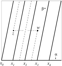
Figure 1. A Heegaard diagram for the lens space $L(5,1)$, and the knot $K(5,1,2)$ within it. The horizontal line segment has been pushed slightly into the alpha handlebody.

The disks $A=\{0\}\times D_{\alpha}$ and $B=\{0\}\times D_{\beta}$ intersect at $p$ points along their boundaries; these are the places where $\alpha$ intersects $\beta$ in the Heegaard diagram. We label these points $x_{0},x_{1},\ldots,x_{p-1}$ in order of their appearance on $\alpha$, as shown in Figure 1.

Definition 2.4.

[5] The simple knot $K(p,q,k)\subset L(p,q)$ is the oriented knot which is the union of an arc joining $x_{0}$ to $x_{k}$ in $A$ with an arc joining $x_{k}$ to $x_{0}$ in $B$.

In the above definition, it is most convenient to take $p>0$, and view $q$ and $k$ as elements of ${\mathbb{Z}}/p$. Note that by translating the fundamental domain of the Heegaard torus, we could just as well have used $x_{i}$ and $x_{i+k}$, for any $i\in{\mathbb{Z}}/p$.

To draw $K(p,q,k)$ in the Heegaard diagram, we replace the disks $A$ and $B$ by translates $A^{\prime}=\{x\}\times D_{\alpha}$ and $B^{\prime}=\{y\}\times D_{\beta}$, so that $x_{i}$ and $x_{i+k}$ are replaced by translates ${z}=x_{i}^{\prime}$ and ${w}=x_{i+k}^{\prime}$. To get the knot, we join ${z}$ to ${w}$ by a horizontal segment in $S^{1}\times D^{2}_{\alpha}$ and ${w}$ to ${z}$ by a segment of slope $p/q$ in $S^{1}\times D^{2}_{\beta}$, as illustrated in Figure 1. Equivalently, as described in [27] the knot $K(p,q,k)$ is derived from the doubly-pointed Heegaard diagram $(T^{2},\alpha,\beta,{z},{w})$.

Lemma 2.5.

We have the following relations among the $K(p,q,k)$:

1. $K(p,q,-k)$ is the orientation-reverse of $K(p,q,k)$.

2. $K(p,-q,-k)$ is the mirror image of $K(p,q,k)$ in $\overline{L(p,q)}=L(p,-q)$.

3. $K(p,q,k)\cong K(p,q^{\prime},kq^{\prime})$, where $qq^{\prime}\equiv 1\ (p)$.

Proof.

The first two identifications are elementary. For the third, observe that the identification $L(p,q)\cong L(p,q^{-1})$ can be obtained by exchanging the roles of $\alpha$ and $\beta$ in the Heegaard diagram. As we travel along the (original) beta curve, we encounter the $x_{i}$’s in the following order: $x_{0},x_{q},x_{2q},\ldots x_{(p-1)q}$. The point $x_{k}$ is in the $q^{\prime}k$-th position in this list. ∎

We would like to know when the knot $K=K(p,q,k)$ admits a homology sphere surgery. To determine its homology class, note that $K$ is homotopic to an immersed curve in the Heegaard torus. The image of $[K]$ in $H_{1}(S^{1}\times D^{2}_{\beta})$ is given by $[K]\cdot\beta=k$, so $[K]=k[b]$, where $b=S^{1}\times\{0\}\subset S^{1}\times D_{\beta}$ is the core curve of the beta handlebody. Thus $[K]$ generates $H_{1}(L(p,q))$ precisely when $k$ is relatively prime to $p$.

To compute the self-linking number of $K$, we observe that $[b]\cdot[b]\equiv q^{\prime}/p\ \text{mod}\ 1$. Thus $K\cdot K\equiv k^{2}q^{\prime}/p\ \text{mod}\ 1$. Now if $k^{2}q^{\prime}\equiv\pm 1\ (p)$, then $k$ must be relatively prime to $p$, so $K(p,q,k)$ is a primitive knot in $L(p,q)$. In summary, we have proved

Lemma 2.6.

The knot $K(p,q,k)$ has an integer surgery which is a homology sphere if and only if $k^{2}\equiv\pm q\ (p)$.

3. Knot Floer homology

In this section, we briefly review the theory of knot Floer homology for rationally null-homologous knots, as developed by Ozsváth and Szabó in [24]. With the exception of Proposition 3.1, all of this material may be found in [24] (c.f [27], [31].) To keep things simple, we will focus on the case where $K$ is a primitive knot of order $p$ in a rational homology sphere $Z$.

3.1. Heegaard diagrams

Any knot $K\subset Z$ can be represented by a doubly pointed Heegaard diagram $(\Sigma,\mbox{\boldmath$\alpha$},\mbox{\boldmath$\beta$},{z},{w})$, as illustrated in Figure 1b. Here $\Sigma$ is a surface of genus $g$, and ${\mbox{\boldmath$\alpha$}}=\{\alpha_{1},\ldots,\alpha_{g}\}$ and ${\mbox{\boldmath$\beta$}}=\{\beta_{1},\ldots,\beta_{g}\}$ are two sets of attaching circles on $\Sigma$. In other words, $\alpha_{1},\alpha_{2},\ldots\alpha_{g}$ are embedded, disjoint, simple closed curves on $\Sigma$ which are linearly independent in $H_{1}(\Sigma)$, and similarly for the $\beta_{i}$. The triple $(\Sigma,{\mbox{\boldmath$\alpha$}},{\mbox{\boldmath$\beta$}})$ is a Heegaard diagram for $Z$, i.e. $\Sigma$ is a Heegaard surface for $Z$ so that the $\alpha_{i}$’s bound compressing disks in one handlebody bounding $\Sigma$, and the $\beta_{i}$’s bound compressing disks in the other.

The knot $K$ is specified by the two basepoints ${z}$ and ${w}$ in $\Sigma-{\mbox{\boldmath$\alpha$}}-{\mbox{\boldmath$\beta$}}$ by the following rule: we join ${z}$ to ${w}$ by an arc in $\Sigma$ which is disjoint from $\alpha$ and push it slightly into the alpha handlebody, Similarly, we join ${w}$ to ${z}$ by an arc in $\Sigma$ which is disjoint from $\beta$ and push this arc slightly into the beta handlebody. $K$ is the union of these two arcs.

Given such a doubly-pointed diagram, we can construct a Heegaard diagram for the complement of a regular neighborhood of $K$ as follows. First, we remove small neighborhoods of ${z}$ and ${w}$ from $\Sigma$. We then join the resulting boundaries by a tube to form a new surface $\Sigma^{\prime}$ of genus $g+1$. Finally, we add an additional alpha circle $\alpha_{g+1}$, which runs from $z$ to $w$ in $\Sigma$, and then back over the tube. In the new diagram, the meridian of the knot $K$ is represented by a small circle linking the tube. This process is illustrated for the knot $K(5,1,2)$ in Figure 2.

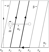
Figure 2. A genus two Heegaard diagram for the complement of $K(5,1,2)$. The heavy lines show the one-chain $\eta(x_{3},x_{1})$.

3.2. Generators

Given a doubly pointed Heegaard diagram $(\Sigma,{\mbox{\boldmath$\alpha$}},{\mbox{\boldmath$\beta$}},{z},{w})$ which represents $K$, Ozsváth and Szabó construct a filtered chain complex $\widehat{CF}(K)$. This complex depends on the doubly pointed Heegaard diagram, but its filtered chain homotopy type is an invariant of $K$.

The generators of $\widehat{CF}(K)$ are easy to describe; they consist of unordered $g$-tuples of intersection points ${\bf x}=\{x_{1},x_{2},\ldots x_{g}\}$ between the alpha and beta curves, such that each alpha and beta curve is represented exactly once. To be precise, each $x_{i}$ is in $\alpha_{j}\cap\beta_{k}$ for some $j$ and $k$, and each $\alpha_{j}$ and $\beta_{k}$ contains exactly one $x_{i}$. More geometrically, the generators correspond to the intersection points of two half-dimensional tori $\mathbb{T}_{\alpha}$, $\mathbb{T}_{\beta}$ in the symmetric product $\text{Sym}^{g}\Sigma$. For this reason, the set of generators is usually denoted by $\mathbb{T}_{\alpha}\cap\mathbb{T}_{\beta}$. Each generator has a ${\mathbb{Z}}/2$ valued homological grading, which is given by the sign of the corresponding intersection between $\mathbb{T}_{\alpha}$ and $\mathbb{T}_{\beta}$. Example: The simple knot $K(p,q,k)$ can be represented by a doubly pointed diagram of genus one, as described in section 2.1. With respect to this diagram, the generators of $\widehat{CF}(K(p,q,k))$ are just the $p$ intersection points $x_{0},x_{1},\ldots,x_{p-1}$ between $\alpha$ and $\beta$. All of these intersection points have the same sign.

3.3. $\text{spin}^{c}$ structures and the Alexander grading

In order to describe the differential on $\widehat{CF}(K)$, we must introduce some more notation. The alpha and beta curves define a cellulation of $\Sigma$. The vertices of this cellulation are the intersection points $\alpha_{j}\cap\beta_{k}$, the one-cells are arcs on the $\alpha_{j}$ and $\beta_{k}$, and the two-cells are the components of $\Sigma-{\mbox{\boldmath$\alpha$}}-{\mbox{\boldmath$\beta$}}$.

Given two generators ${\bf x}$ and $\bf y$, we can construct a one-chain $\eta({\bf x},{\bf y})$ by going from points in ${\bf x}$ to points in ${\bf y}$ along the alpha curves, and then from points in ${\bf y}$ back to points in ${\bf x}$ along the beta curves. We can change $\eta({\bf x},{\bf y})$ by adding copies of the $\alpha_{i}$’s and $\beta_{j}$’s to it, but it has a well-defined image $\epsilon({\bf x},{\bf y})$ in $H_{1}(\Sigma)/\langle\alpha_{1},\dots,\alpha_{g},\beta_{1},\ldots,\beta_{g}\rangle\cong H_{1}(Z).$ This $\epsilon$-grading is additive, in the sense that

$$\epsilon({\bf x},{\bf y})+\epsilon({\bf y},{\bf z})=\epsilon({\bf x},{\bf z}).$$

We define an equivalence relation on the set of generators by setting ${\bf x}\sim{\bf y}$ if $\epsilon({\bf x},{\bf y})=0$. The set of equivalence classes is an affine set isomorphic to $H_{1}(Z)$.

If we fix a basepoint $q\in\Sigma-\mbox{\boldmath$\alpha$}-\mbox{\boldmath$\beta$}$, the set of equivalence classes can naturally be identified with the set of $\text{spin}^{c}$ structures on $Z$. We write $\mathfrak{s}_{q}({{{\bf x}}})$ to denote the $\text{spin}^{c}$ structure determined by the pair $(q,{{{\bf x}}})$. Varying $q$ changes $\mathfrak{s}_{q}({{{\bf x}}})$ according to the formula

(1) $$\mathfrak{s}_{q_{1}}({{{\bf x}}})-\mathfrak{s}_{q_{2}}({{{\bf x}}})=[K_{q_{1},q_{2}}],$$

where $K_{q_{1},q_{2}}$ is the oriented knot determined by the pair of basepoints $(q_{1},q_{2})$.

In the presence of a knot, we can define an enhancement of the $\epsilon$-grading known as the Alexander grading. To do this, we consider the same one-chain $\eta({\bf x},{\bf y})$, but in the Heegaard diagram for the knot complement. The image of $\eta({\bf x},{\bf y})$ defines a well defined element

$$A({\bf x},{\bf y})\in H_{1}(\Sigma^{\prime})/\langle\alpha_{1},\ldots,\alpha_{g},\alpha_{g+1},\beta_{1},\ldots,\beta_{g}\rangle\cong H_{1}(Z-K).$$

Like the $\epsilon$–grading, the Alexander grading is an additive function. It reduces to the $\epsilon$–grading under the homomorphism $H_{1}(Z-K)\to H_{1}(Z)$. If $K$ is a primitive knot of order $p$ (so $H_{1}(Z-K)\cong{\mathbb{Z}}$), this means that two generators belong to the same $\text{spin}^{c}$ structure if and only if their Alexander gradings are congruent modulo $p$.

Example: Consider the diagram of $K=K(5,1,2)$ in Figure 2. A suitable one-chain $\eta(x_{3},x_{1})$ is shown in bold in the figure. By inspection, we see that $\epsilon(x_{3},x_{1})=2a$, where $a$ is the class of the vertical loop at the left-hand side of the figure. More generally, we have $\epsilon(x_{i},x_{j})=(i-j)a$. Since $a$ generates $H_{1}(L(5,1))$, the generators $x_{0},\dots,x_{4}$ all belong to different $\text{spin}^{c}$ structures. The same argument shows that if $K=K(p,q,k)$, the generators $x_{0},\ldots,x_{p-1}$ all represent different $\text{spin}^{c}$ structures.

To compute the Alexander grading $A(x_{3},x_{1})$, we consider the image of the same loop, but in the group $H_{1}(Z-K)\cong H_{1}(\Sigma^{\prime})/\langle\alpha_{1},\alpha_{2},\beta\rangle$. The quotient $H_{1}(\Sigma^{\prime})/\langle\alpha_{1},\alpha_{2}\rangle$ is generated by $a$ and $m$, and the image of $\beta$ in this quotient is $5a+2m$. Thus $H_{1}(Z-K)$ is generated by an element $x$ with $a=2x$ and $m=-5x$. $\eta(x_{3},x_{1})$ is homologous to $2a+2m$, so $A(x_{3},x_{1})=-6x$.

3.4. Domains

If ${\bf x}$ and ${\bf y}$ are two generators, we define $\pi_{2}({\bf x},{\bf y})$ (the set of domains from ${\bf x}$ to ${\bf y}$) to be the set of two-chains $\phi$ with the property that $\partial\phi=\eta({\bf x},{\bf y})$ for some one-chain $\eta({\bf x},{\bf y})$ joining ${\bf x}$ and ${\bf y}$. Thus $\pi_{2}({\bf x},{\bf y})$ is empty unless ${\bf x}$ and ${\bf y}$ belong to the same $\text{spin}^{c}$ structure. In the latter case, assuming that $Z$ is a rational homology sphere, there is a unique choice of $\eta$ which bounds a two-chain in $\Sigma$. Thus $\pi_{2}({\bf x},{\bf y})$ is an affine copy of ${\mathbb{Z}}$, where the action of ${\mathbb{Z}}$ is given by adding multiples of $\Sigma$.

If $\phi\in\pi_{2}({\bf x},{\bf y})$ and $q\in\Sigma-\mbox{\boldmath$\alpha$}-\mbox{\boldmath$\beta$}$, then $\phi$ has a well-defined multiplicity $n_{q}(\phi)$ at $q$. When ${\bf x}$ and ${\bf y}$ belong to the same $\text{spin}^{c}$ structure, their Alexander gradings are related by the following formula:

(2) $$A({\bf x},{\bf y})=p(n_{w}(\phi)-n_{z}(\phi))$$

for any $\phi\in\pi_{2}({\bf x},{\bf y})$.

3.5. The Floer chain complex

We are now in a position to describe the differential on $\widehat{CF}(K)$. It takes the following form:

$$d{\bf x}=\sum_{{\bf y}\in\mathbb{T}_{\alpha}\cap\mathbb{T}_{\beta}}\quad\sum_{{\{\phi\in\pi_{2}({\bf x},{\bf y}){{\thinspace}}|{{\thinspace}}n_{z}(\phi)=0\}}}M(\phi){\bf y}.$$

The function $M(\phi)$ is defined by counting certain pseudo-holomorphic maps associated to the domain $\phi$. For a precise formulation of this count in two different contexts, see [28], [19]; the main thing that we will need to know about it is that $M(\phi)=0$ unless $n_{q}(\phi)\geq 0$ for every $q\in\Sigma-\mbox{\boldmath$\alpha$}-\mbox{\boldmath$\beta$}$. (Such a $\phi$ is called a positive domain.)

Regarding the form of the differential, note that the inner sum is empty unless ${\bf x}$ and ${\bf y}$ belong to the same $\text{spin}^{c}$ structure. In this case, there is a unique element $\phi_{0}({\bf x},{\bf y})\in\pi_{2}({\bf x},{\bf y})$ with $n_{z}(\phi_{0})=0$, so the formula for the differential can be rewritten as

$$d{\bf x}=\sum_{{\bf y}\sim{\bf x}}M(\phi_{0}({\bf x},{\bf y})){\bf y}.$$

In particular, we can decompose $\widehat{CF}(K)$ into a direct sum over $\text{spin}^{c}$ structures:

$$\widehat{CF}(K)\cong\bigoplus_{\mathfrak{s}\in\text{Spin}^{c}(Z)}\widehat{CF}(K,\mathfrak{s}).$$

Example: If we represent $K=K(p,q,k)$ by a genus one Heegaard diagram as in Figure 2, then $\widehat{CF}(K,\mathfrak{s})\cong{\mathbb{Z}}$ for each $\mathfrak{s}\in\text{Spin}^{c}(L(p,q))$. Since each generator belongs to a different $\text{spin}^{c}$ structure, there are no differentials in the complex $\widehat{CF}(K)$.

3.6. The knot filtration

Up to this point, we have not made much use of the knot $K$. Indeed, the homology of the complex $\widehat{CF}(K)$ is just the ordinary Heegaard Floer homology ${{\widehat{HF}}}(Z)$ as defined in [28]. To put $K$ into the picture, we observe that if $M(\phi_{0}({\bf x},{\bf y}))\neq 0$, then $n_{w}(\phi_{0}({\bf x},{\bf y}))\geq 0$. From equation 2, it follows that $A({\bf x},{\bf y})\geq 0$ as well. For ease of notation, let us pass (somewhat arbitrarily) from an affine $H_{1}(Z-K)$ grading to an actual $H_{1}(Z-K)$ grading by fixing some generator ${\bf x_{0}}$ and setting $A({\bf x})=A({\bf x},{\bf x_{0}})$. (In the next section, we will see that there is a canonical way to do this.) Then the formula for the differential becomes

$$d{\bf x}=\sum_{\{{\bf y}{{\thinspace}}|{{\thinspace}}A({\bf y})\leq A({\bf x})\}}M(\phi_{0}({\bf x},{\bf y})){\bf y}.$$

In other words, the Alexander grading defines a filtration on $\widehat{CF}(K)$. The associated graded complex $\widehat{CF}(K,j)$ is generated by those ${{{\bf x}}}$ with $A({{{\bf x}}})=j$. Its homology is denoted by $\widehat{HFK}(K,j)$ or (if we sum over all $j\in{\mathbb{Z}}$) by $\widehat{HFK}(K)$, and is called the knot Floer homology. When we need it, the ${\mathbb{Z}}/2$ homological grading is indicated by a subscript: $\widehat{HFK}_{i}(K,j)$.

3.7. Fox Calculus and the Alexander polynomial

The Fox calculus [11], [8] provides a streamlined method for computing the Alexander grading. We briefly sketch this relationship here; for more details, see chapter 2 of [31].

We start with the Heegaard diagram $(\Sigma^{\prime},\mbox{\boldmath$\alpha$}^{\prime},\mbox{\boldmath$\beta$})$ for $Z-K$ described in section 3.1. Any such diagram gives rise to a presentation of $\pi_{1}(Z-K)$ as follows. First, we choose orientations for the alpha and beta curves. We associate a generator $a_{i}$ to each $\alpha_{i}$, and a relation $w_{j}$ to each $\beta_{j}$, according to the following rule. Starting at an arbitrary point of $\beta_{j}$ and with the empty word $w$, we transverse the curve, recording each intersection with an alpha curve (say $\alpha_{k}$) by appending $a_{k}^{\pm 1}$ to $w$, where the sign is determined by the sign of the intersection between $\alpha_{k}$ and $\beta_{j}$.

Let $|\cdot|:\pi_{1}(Z-K)\to H_{1}(Z-K)$ denote the abelianization map. For any word $w$ in the $a_{i}$, we define the free differential $d_{a_{i}}w$ to be an element of the group ring ${\mathbb{Z}}[H_{1}(Z-K)]$ determined by the following rules:

$$d_{a_{i}}a_{j} =\delta_{ij}$$

$$d_{a_{i}}(ab) =d_{a_{i}}a+t^{|a|}d_{a_{i}}b$$

$$d_{a_{i}}a^{-1} =-t^{|a|}d_{a_{i}}a.$$

(In fact, the last rule is a consequence of the preceding two.)

Before we combine terms, the expression $d_{a_{i}}w_{j}$ contains one monomial for each point in $\alpha_{i}\cap\beta_{j}$. If we formally expand the expression $\det(d_{a_{i}}w_{j})_{1\leq i,j\leq g}$, again without combining terms, we obtain a polynomial with one term for each generator of the complex $\widehat{CF}(K)$.This polynomial encodes the Alexander grading, in the sense that if ${\bf x}$ and ${\bf y}$ correspond to monomials $\pm t^{x}$ and $\pm t^{y}$, then $A({\bf x},{\bf y})=x-y$. It also encodes the ${\mathbb{Z}}/2$ homological grading: if two generators have the same ${\mathbb{Z}}/2$ grading, the corresponding monomials have the same sign, and if the gradings are opposite, their monomials have opposite signs.

Combining terms in this expression corresponds to the operation of taking the graded Euler characteristic. More precisely, we have

$$\chi(\widehat{HFK}(K)) =\sum_{i,j}(-1)^{i}t^{j}\dim\widehat{HFK}_{i}(K,j)$$

$$=\sum_{{\bf x}\in\mathbb{T}_{\alpha}\cap\mathbb{T}_{\beta}}(-1)^{{{\mathrm{gr}}}({\bf x})}t^{A({\bf x})}$$

$$=\det(d_{a_{i}}w_{j})_{1\leq i,j\leq g}.$$

The matrix $A=(d_{a_{i}}w_{j})$, where $1\leq i\leq g+1$ and $1\leq j\leq g$, is known as the Alexander matrix. The Alexander polynomial $\Delta_{K}(t)$ is defined to be the $\gcd$ of its $g\times g$ minors.

Proposition 3.1.

Let $K\subset Z$ be a primitive knot of order $p$. Then

$$\chi(\widehat{HFK}(K))\sim\Delta_{K}(t)\cdot\frac{t^{p}-1}{t-1}.$$

Here we write $f\sim g$ to indicate $f=\pm t^{k}g.$ (This ambiguity arises because the $\gcd$ is only well defined up to multiplication by $\pm t^{k}$.)

Proof.

In light of our comments above, this amounts to showing that

$$\det(d_{a_{i}}w_{j})_{1\leq i,j\leq g}\sim\Delta_{K}(t)\cdot\frac{t^{p}-1}{t-1}.$$

That this is true was certainly known to Fox (c.f. item 6.3 of [12]), who actually attributes it to Alexander [1]. Since the proof is perhaps less well-known to a modern audience, we sketch it here. The rows of the Alexander matrix form $g+1$ vectors ${\bf v}_{1},{\bf v}_{2},\ldots{\bf v}_{g+1}$ in a $g$-dimensional space, so there must be a linear relation between them. This relation is given by Fox’s fundamental formula, which implies that for any word $w$

$$t^{|w|}-1=\sum_{i=1}^{g+1}d_{a_{i}}w\cdot(t^{|a_{i}|}-1).$$

(In fact, an analogous relation holds in the group ring of the free group as well.) When $w$=$w_{j}$ is a relation in $\pi_{1}(Z-K)$, the left-hand side of this equation is $0$. It follows that the ${\bf v}_{i}$ satisfy the equation

$$\sum_{i=1}^{g+1}(t^{|a_{i}|}-1){\bf v}_{i}=0.$$

Let $\Delta_{i}$ be the determinant of the $g\times g$ matrix obtained by deleting the $i$-th row of $A$. By solving for ${\bf v}_{j}$ in the above equation and substituting it into the expression for $\Delta_{i}$, we find that

$$\frac{\Delta_{i}}{\Delta_{j}}=\pm\frac{t^{|a_{i}|}-1}{t^{|a_{j}|}-1}.$$

Since the $a_{i}$ generate $\pi_{1}(Z-K)$, their abelianizations generate $H_{1}(Z-K)\cong{\mathbb{Z}}$. In other words, $\gcd(|a_{i}|)=1$, which implies that $\gcd(t^{|a_{i}|}-1)=t-1$. Knowing this, it is not difficult to see that

$$\Delta_{i}\sim\Delta_{K}(t)\cdot\frac{t^{|a_{i}|}-1}{t-1}.$$

The desired formula is a special case, since $|a_{g+1}|=|m|=\pm p$. ∎

It is a well-known fact that the Alexander polynomial $\Delta_{K}(t)$ can be normalized so that $\Delta_{K}(t^{-1})=\Delta_{K}(t)$, $\Delta_{K}(1)=1$. We use this normalization to fix particular values for the Alexander and homological gradings on $\widehat{CF}(K)$, by requiring that

$$\chi(\widehat{HFK}(K))=\overline{\Delta}(K)=\Delta_{K}(t)\cdot\frac{t^{p/2}-t^{-p/2}}{t^{1/2}-t^{-1/2}}.$$

is a symmetric Laurent polynomial with $\overline{\Delta}_{K}(1)=p$.

Example: Let $K=K(5,1,2)$. Referring to the diagram in Figure 2, we let $a$ be the generator of $\pi_{1}(Z-K)$ corresponding to $\alpha_{1}$, and $m$ be the generator corresponding to $\alpha_{2}$. If we traverse $\beta$ starting just below the point $x_{1}$, we find that the corresponding relator is $w=amama^{3}$. The abelianization map $|\cdot|:\pi_{1}(Z-K)\to H_{1}(Z-K)$ satisfies $|a|=2$, $|m|={-5}$, so

$$d_{a}w =1+t^{|am|}+t^{|amam|}+t^{|amama|}+t^{|amama^{2}|}$$

$$=1+t^{-3}+t^{-6}+t^{-4}+t^{-2}.$$

Thus

$$\overline{\Delta}(K)=t^{-3}+t^{-1}+1+t+t^{3}$$

and the Alexander gradings of $x_{1},x_{2},x_{3},x_{4}$, and $x_{0}$ are $3,0,-3,-1,$ and $1$ respectively. The Alexander polynomial of $K$ is

$$\Delta_{K}(t)\sim\frac{(t-1)d_{a}(w)}{t^{5}-1}\sim t^{-1}-1+t$$

This is recognizable as the Alexander polynomial of the trefoil knot in $S^{3}$. In fact, $Z=L(5,1)$ is realized by $-5$ surgery on the trefoil, and $K$ is the dual knot in $Z$.

3.8. Reversing orientation

We now consider the effect of exchanging the roles of $z$ and $w$ in the definition of $\widehat{CF}(K)$, so that instead of considering domains with $n_{z}(\phi)=0$, we use domains with $n_{w}(\phi)=0$. Switching the basepoints has the effect of reversing the orientation on $K$, so we denote the resulting complex by $\widehat{CF}(-K)$. This complex has the same generators as $\widehat{CF}(K)$, but the differentials are different. From equation (2), we see that the Alexander grading defines an increasing filtration on $\widehat{CF}(-K)$, i.e. $d{\bf x}$ is a sum of generators ${\bf y}$ with $A({\bf y})\geq A({\bf x})$.

The $\epsilon$-grading on $\widehat{CF}(-K)$ remains the the same as on $\widehat{CF}(K)$, but the $\text{spin}^{c}$ structure determined by an equivalence class will differ. In order to state the relationship precisely, we denote by $\mathfrak{s}_{k}$ the $\text{spin}^{c}$ structure on $Z$ given by $\mathfrak{s}_{z}({\bf x})$, where ${\bf x}$ is any generator with $A(k)\equiv k\ (p)$. Then by combining Lemma 2.3 with equation (1), we see that

$$\mathfrak{s}_{w}({\bf x}) =\mathfrak{s}_{z}({\bf x})-[K]$$

$$=\mathfrak{s}_{A(x)-a},$$

where $a$ is the self-linking number of $K$. In particular, the summand of $\widehat{CF}(-K)$ generated by those ${\bf x}$ with $A({\bf x})\equiv k\ (p)$ has homology equal to ${{\widehat{HF}}}(Z,\mathfrak{s}_{k-a})$.

4. Knots with LHS surgeries

We now suppose that we are given a knot $K\subset Z$, where $Z$ is an L-space. In this section, we give a precise characterization of when $K$ has a surgery which is an L-space homology sphere in terms of the knot Floer homology of $K$. The main tool is the mapping cone theorem of Ozsváth and Szabó [24], which expresses the Heegaard Floer homology of surgeries on $K$ in terms of the homology of certain complexes derived from $\widehat{CF}(K)$ and $\widehat{CF}(-K)$. We begin by recalling their construction.

4.1. The complex $C_{n}(K)$

The differential in the complex $\widehat{CF}(K)$ can be decomposed as $d=d_{0}+d_{+}$, where

$$d_{0}({\bf x}) =\sum_{A({\bf y})=A({\bf x})}\quad\sum_{\{\phi\in\pi_{2}({\bf x},{\bf y}){{\thinspace}}|{{\thinspace}}n_{z}(\phi)=n_{w}(\phi)=0\}}M(\phi){\bf y}$$

$$d_{+}({\bf x}) =\sum_{A({\bf y})<A({\bf x})}\quad\sum_{\{\phi\in\pi_{2}({\bf x},{\bf y}){{\thinspace}}|{{\thinspace}}n_{z}(\phi)=0\}}M(\phi){\bf y}$$

Similarly, the differential in $\widehat{CF}(-K)$ can be decomposed as $d_{0}+d_{-}$, where

$$d_{-}({\bf x})=\sum_{A({\bf y})>A({\bf x})}\quad\sum_{\{\phi\in\pi_{2}({\bf x},{\bf y}){{\thinspace}}|{{\thinspace}}n_{z}(\phi)=0\}}M(\phi){\bf y}$$

For each $n\in{\mathbb{Z}}$, we let $C_{n}(K)$ be the complex generated by those ${{{\bf x}}}\in\mathbb{T}_{\alpha}\cap\mathbb{T}_{\beta}$ for which $A({\bf x})\equiv n\ (p)$, and whose differential is given by the formula

$$d_{n}{\bf x}=\begin{cases}d_{0}({\bf x})+d_{+}({\bf x})&\quad\text{if}\ A({\bf x})<n\\ d_{0}({\bf x})+d_{+}({\bf x})+d_{-}({\bf x})&\quad\text{if}\ A({\bf x})=n\\ d_{0}({\bf x})+d_{-}({\bf x})&\quad\text{if}\ A({\bf x})>n.\end{cases}$$

When $n\gg 0$, $C_{n}(K)=\widehat{CF}(K,\mathfrak{s}_{n})$, while for $n\ll 0$ , $C_{n}(K)=\widehat{CF}(-K,\mathfrak{s}_{n-a})$. There are natural maps $\pi_{n}^{+}:C_{n}(K)\to\widehat{CF}(K,\mathfrak{s}_{n})$ and $\pi_{n}^{-}:C_{n}(K)\to\widehat{CF}(-K,\mathfrak{s}_{n-a})$ defined by

$$\pi_{n}^{+}({\bf x})=\begin{cases}{\bf x}&\quad\text{if}\ A({\bf x})\leq n\\ 0&\quad\text{if}\ A({\bf x})>n\end{cases}\quad\text{and}\quad\pi_{n}^{-}({\bf x})=\begin{cases}0&\quad\text{if}\ A({\bf x})<n\\ {\bf x}&\quad\text{if}\ A({\bf x})\geq n.\end{cases}$$

We denote the homology group $H(C_{n}(K),d_{n})$ by $A_{n}$, and let

$$\pi_{n}^{+}:A_{n}\to{{\widehat{HF}}}(Z,\mathfrak{s}_{n})\quad\text{and}\quad\pi_{n}^{-}:A_{n}\to{{\widehat{HF}}}(Z,\mathfrak{s}_{n-a})$$

be the induced maps.

Geometrically speaking, the group $A_{n}$ can be identified with ${{\widehat{HF}}}(Z^{\prime},\mathfrak{s}_{n})$, where $Z^{\prime}$ is a manifold obtained by doing a large integral surgery on $K$, and $\mathfrak{s}_{n}$ is a particular $\text{spin}^{c}$ structure on $Z^{\prime}$ (c.f. section 4 of [24]). The maps $\pi_{n}^{\pm}$ are induced by certain $\text{spin}^{c}$ structures on the surgery cobordism. An easy (but useful) consequence of this identification is that each $A_{n}$ must have rank $\geq 1$.

4.2. The mapping cone formula

The formula of [24] expresses the homology of surgeries on $K$ in terms of the groups $A_{n}$ and their projections $\pi_{n}^{\pm}$ to ${{\widehat{HF}}}(Z)$. To be precise, recall from Lemma 2.3 that the first homology groups of the manifolds $K_{m}$ obtained by integer surgery on $K$ are precisely of the form ${\mathbb{Z}}/m$, where $m\equiv-a\ (p)$.

We now fix some $m\equiv-a\ (p)$. For each $n\in{\mathbb{Z}}$, we define $B_{n}={{\widehat{HF}}}(Z,\mathfrak{s}_{n})$. (Note that although $B_{n_{1}}\cong B_{n_{2}}$ whenever $n_{1}\equiv n_{2}\ (p)$, we treat them as different groups.) Then we have maps

$$\pi_{n}^{+} :A_{n}\to B_{n}$$

$$\pi_{n}^{-} :A_{n}\to B_{n+m}.$$

We write

$$A=\bigoplus_{n\in{\mathbb{Z}}}A_{n}\quad\text{and}\quad B=\bigoplus_{n\in{\mathbb{Z}}}B_{n}.$$

and let $\pi^{\pm}:A\to B$ be the maps whose components are given by $\pi^{\pm}_{n}$. Then we can form the short chain complex

$$\begin{CD}C(K,m)=A@>{\pi^{-}+\pi^{+}}>{}>B.\end{CD}$$

Theorem 4.1.

[24] ${{\widehat{HF}}}(K_{m})$ is isomorphic to the homology of the complex $C(K,m)$.

A few remarks are in order. First, we should point out that the homology of the complexes $\widehat{CF}(K,\mathfrak{s}_{n})$ and $\widehat{CF}(-K,\mathfrak{s}_{n})$ both compute ${{\widehat{HF}}}(Z,\mathfrak{s}_{n})$, so they are canonically isomorphic (c.f. Theorem 2.1 of [30]). In general, however, there is no easy way to determine this isomorphism. Thus even though the maps $\pi^{+}$ and $\pi^{-}$ are determined by the complex $\widehat{CF}(K)$, the behavior of their sum can be quite difficult to calculate. However, we will only consider the case where ${{\widehat{HF}}}(Z,\mathfrak{s}_{n})\cong{\mathbb{Z}}$ (which has very few isomorphisms), so this difficulty will not arise.

Second, note that since $\pi^{+}$ preserves $n$, and $\pi^{-}$ raises it by $m$, $C(K,m)$ can be decomposed into a direct sum of $m$ complexes. This splitting corresponds to the decomposition of ${{\widehat{HF}}}(K_{m})$ into $\text{spin}^{c}$ structures.

Finally, observe that for $n\gg 0$, the map $\pi_{n}^{-}$ is trivial, and $\pi_{n}^{+}$ is an isomorphism. Similarly, for $n\ll 0$, $\pi_{n}^{-}$ is an isomorphism, and $\pi_{n}^{+}$ is trivial. It follows that the chain complex $C(K,m)$ (which is infinitely generated) can be decomposed into an infinite number of summands of the form

$$\begin{CD}A_{n}@>{\pi_{n}^{+}}>{}>B_{n}\quad(n>N_{+})\quad\text{and}\quad A_{n}@>{\pi_{n}^{-}}>{}>B_{n+m}\quad(n<N_{-})\end{CD}$$

whose homology is trivial, together with a single interesting summand $\widetilde{C}(K,m)$ which contains $A_{n}$ for $N_{-}\leq n\leq N_{+}$ and $B_{n}$ for $N_{-}+m\leq n\leq N_{+}$.

4.3. Proof of Theorem 1

Suppose now that $Z$ is an L-space. We wish to characterize when $K$ has an L-space homology sphere surgery in terms of $\widehat{HFK}(K)$. To do so, we recall a few invariants derived from the knot Floer homology.

Definition 4.2.

The width of $\widehat{HFK}(K)$ is the difference $M_{+}-M_{-}$, where $M_{+}$ is the maximum value of $j$ for which $\widehat{HFK}(K,j)$ is nontrivial, and $M_{-}$ is the minimum value.

The width is related to the genus of $K$ by the following theorem of Ni:

Theorem 4.3.

[22] Suppose $K$ is a primitive knot in a rational homology sphere $Z$, and that $H_{1}({\mathbb{Z}})\cong{\mathbb{Z}}/p$. Then $g(K)=(\text{\em{width}}\ \widehat{HFK}(K)-p+1)/2$.

The other invariant is an obvious generalization of the Ozsváth-Szabó $\tau$ invariant defined in [26] (c.f. [16], [31]):

Definition 4.4.

If $\mathfrak{s}_{k}$ is a $\text{spin}^{c}$ structure on $Z$, we define $\tau(K,\mathfrak{s}_{k})$ to be the minimum value of $n\equiv k\ (p)$ for which the map $\pi^{+}_{n}$ is nontrivial.

Proposition 4.5.

Suppose $Z$ is an L-space, and that $K\subset Z$ has a homology sphere surgery $Y$. Then $Y$ is an L-space if and only if one of the following conditions holds:

1. $\widehat{HFK}(K)\cong{\mathbb{Z}}^{p}$ and $\text{\em width}\ \widehat{HFK}(K)<2p$.

2. $\widehat{HFK}(K)\cong{\mathbb{Z}}^{p+2}$, $\text{\em width}\ \widehat{HFK}(K)=2p$, and either $Y=K_{1}$ and $\tau(K,\mathfrak{s}_{0})>0$ or $Y=K_{-1}$ and $\tau(K,\mathfrak{s}_{0})<0$.

We will work our way up to the proof through a series of lemmas. For the rest of this section, we suppose that $Z$ is an L-space and that $K\subset Z$ admits a homology sphere surgery. For the moment, we assume that this surgery is $K_{1}$.

Lemma 4.6.

If $K_{1}$ is an L-space, then $A_{n}\cong{\mathbb{Z}}$ for every $n\in{\mathbb{Z}}$, and there is at most one value of $n$ for which both $\pi_{n}^{+}$ and $\pi_{n}^{-}$ are both trivial.

Proof.

Since $Z$ is an L-space, $B_{n}\cong{\mathbb{Z}}$ for every $n\in{\mathbb{Z}}$. Thus $A_{n}\cong B_{n}\cong{\mathbb{Z}}$ for all $n>N_{+}$ and $A_{n}\cong B_{n+1}\cong{\mathbb{Z}}$ for all $n<N_{-}$. For the intermediate values of $n$, we consider the complex $\widetilde{C}(K,1)$. The first term in this complex is the direct sum of the $A_{n}$ for $N_{-}\leq n\leq N_{+}$, while the second term is the direct sum of the $B_{n}$ for $N_{-}+1\leq n\leq N_{+}$. In particular, the first term has one more summand than the second. Now each $A_{n}$ has rank $\geq 1$, and each $B_{n}$ has rank $1$. On the other hand, we have

$$H(\widetilde{C}(K,1))\cong H(C(K,1))\cong{{\widehat{HF}}}(K_{1})\cong{\mathbb{Z}}$$

since $K_{1}$ is an L-space. The only way this can happen is if $A_{n}\cong{\mathbb{Z}}$ for each $N_{-}\leq n\leq N_{+}$. This proves the first claim. For the second, note that if both $\pi_{n}^{+}$ and $\pi_{n}^{-}$ are trivial for two different values of $n$, then the homology of $\widetilde{C}(K,1)$ must have rank $\geq 2$. ∎

Lemma 4.7.

If $K_{1}$ is an L-space, either $\widehat{HFK}(K)\cong{\mathbb{Z}}^{p}$ or $\widehat{HFK}(K)\cong{\mathbb{Z}}^{p+2}$.

Proof.

Consider the complex $\widehat{CF}(K,\mathfrak{s}_{k})$ generated by those ${\bf x}$ with $A({\bf x})\equiv k\ (p)$. By the previous lemma, we know that the associated homology groups $A_{n}$ ($n\equiv k\ (p)$) are all isomorphic to ${\mathbb{Z}}$. This situation was studied by Ozsváth and Szabó in Lemmas 3.1 and 3.2 of [29]. They show that there is a series of integers $n_{1}<n_{2}<\ldots<n_{2m_{k}-1}$ such that $\widehat{HFK}(K,\mathfrak{s}_{k},n_{j})\cong{\mathbb{Z}}$, and that $\widehat{HFK}(K,\mathfrak{s}_{k},n)$ is trivial for all other values of $n\equiv k\ (p)$. Furthermore, if $y_{j}$ is a generator of the group in Alexander grading $n_{j}$, then

$$d_{+}(y_{2j}) =\pm y_{2j+1}\quad\quad d_{+}(y_{2j+1})=0$$

$$d_{-}(y_{2j}) =\pm y_{2j-1}\quad\quad d_{-}(y_{2j-1})=0.$$

From this, it is easy to see that the maps $\pi_{n}^{\pm}$ are both trivial for all $n_{1}<n<n_{2m_{k}-1}$, $n\equiv k\ (p)$. If $m_{k}>1$, there is at least one such value of $k$, and if $m_{k}>2$, there are more than one. By the preceding lemma, we conclude that $m_{k}=1$ (and thus $\widehat{HFK}(K,\mathfrak{s}_{k})\cong{\mathbb{Z}}$) for all but one value of $k$, and that $m_{k}=2$ (so $\widehat{HFK}(K,\mathfrak{s}_{k})\cong{\mathbb{Z}}^{3}$) for this value, if it exists. ∎

Lemma 4.8.

Suppose $\widehat{HFK}(K)\cong{\mathbb{Z}}^{p}$. Then $K_{1}$ is an L-space if and only if

$$\text{\em{width}}\ \widehat{HFK}(K)<2p.$$

Proof.

The argument in the preceding lemma shows that for each $k\in{\mathbb{Z}}/p$, there is a unique $n_{k}\equiv k{{\thinspace}}(p)$ with $\widehat{HFK}(K,n_{k})\cong{\mathbb{Z}}$, and that all the other groups $\widehat{HFK}(K,n)$ vanish. From this, we see that $A_{n}\cong{\mathbb{Z}}$ for all $n$, and that $\pi_{n}^{+}$ is an isomorphism for all $n\geq n_{k}$, $n\equiv k\ (p)$ and vanishes for all $n<n_{k}$. Similarly, $\pi_{-}^{n}$ is an isomorphism for all $n\leq n_{k}$, $n\equiv k\ (p)$, and vanishes for all $n>n_{k}$.

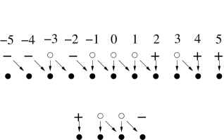
Figure 3. The top half of the figure is a diagram of the complex $\widetilde{C}(K,1)$ for $K=K(5,1,2)$. The numbers label the indices on the groups $A_{n}$ and $B_{n}$, which are indicated by $+$’s, $-$’s and $o$’s (for the $A_{n}$), and solid dots for the $B_{n}$. Summands of type $[-,-]$, $[-,+]$, and $[+,+]$ are visible. The bottom half of the figure shows a typical summand of type $[+,-]$.

We can represent the chain complex $C(K,1)$ by a diagram of the type illustrated in Figure 3. The upper row of the diagram shows the $A_{n}$, while the lower row shows the $B_{n}$. We represent the group $A_{n}$ by a $+$ if $\pi_{n}^{+}$ is nontrivial but $\pi_{n}^{-}=0$, by a $-$ if $\pi_{n}^{-}$ is nontrivial but $\pi_{n}^{+}=0$, and by an $o$ if both maps are nontrivial. (Thus $A_{n_{k}+ip}$ is represented by the sign of $i$.) Each $B_{n}$ is represented by a filled circle. Nontrivial maps are indicated by arrows, but trivial ones are omitted.

The complex $C(K,1)$ can be decomposed into summands corresponding to connected components of the diagram. Each summand corresponds to an interval $[a,b]$, where $a$ and $b$ are labeled with a $+$ or $-$, and all the intervening integers are labeled with an $o$. The homology of a summand of type $[+,+]$ or $[-,-]$ is trivial, but the homology of a summand of type $[-,+]$ is ${\mathbb{Z}}$ (supported in the top row) and the homology of a summand of type $[+,-]$ is ${\mathbb{Z}}$ (supported in the bottom row). Thus there is a unique summand with nontrivial homology if and only if the $-$’s in the diagram appear to the left of all the $+$’s.

Suppose $A_{m}$ is labeled with a $+$, and $A_{n}$ is labeled with a $-$ for some $m<n$. Then $\widehat{HFK}(K,m-ip)\cong{\mathbb{Z}}$ for some $i>0$, and $\widehat{HFK}(K,n+ip)\cong{\mathbb{Z}}$ for some $i>0$, so $\text{width}\ \widehat{HFK}(K)>2p$. Conversely, if $\widehat{HFK}(K,m)\cong\widehat{HFK}(K,n)\cong{\mathbb{Z}}$ with $n-m>2p$, then $A_{m+p}$ is labeled with a $+$ and lies to the left of $A_{n-p}$, which is labeled with a $-$. This proves the claim. ∎

Lemma 4.9.

Suppose $\widehat{HFK}(K)\cong{\mathbb{Z}}^{p+2}$. Then $K_{1}$ is an L-space if and only if

$$\text{{\em width}}\ \widehat{HFK}(K)=2p\quad\text{ and}\quad\tau(K,\mathfrak{s}_{0})>0.$$

Proof.

In this case, there is a unique $\text{spin}^{c}$ structure with $\widehat{HFK}(K,\mathfrak{s})\cong{\mathbb{Z}}^{3}$. The symmetry of $\Delta_{K}(t)$ implies that this is necessarily $\mathfrak{s}_{0}$. If $K_{1}$ is an L-space, the argument used in the proof of Lemma 4.7 shows that the three ${\mathbb{Z}}$ summands are in Alexander gradings $-p,0$, and $p$, and that $\tau(K,\mathfrak{s}_{0})=p$. Conversely, if $\text{{width}}\ \widehat{HFK}(K)=2p$, then $\widehat{HFK}(K,\mathfrak{s}_{0})$ must be supported in Alexander gradings $-p,0$, and $p$. It is now easy to see that $\pi_{ip}^{+}$ is an isomorphism for $i>0$ and vanishes for $i\leq 0$, and that $\pi_{ip}^{-}$ is an isomorphism for $i<0$ and vanishes for $i\geq 0$. All the other $\text{spin}^{c}$ structures behave exactly as they did in the proof of Lemma 4.8.

We represent the chain complex $C(K,1)$ by the same sort of diagram we used in the proof of Lemma 4.8, labeling $A_{0}$ with a $*$, and each $A_{n}$ ($n\neq 0$) by either a $-$, a $+$, or an $o$. As before, $C(K,1)$ decomposes into summands corresponding to intervals $[a,b]$ all of whose interior points are labeled by an $o$; however, there are now some additional possibilities. First, $A_{0}$ itself is always a summand, with homology ${\mathbb{Z}}$. Second, intervals of the form $[-,*]$ and $[*,+]$ correspond to summands with trivial homology, while those of the form $[+,*]$, and $[*,-]$ have homology ${\mathbb{Z}}$. From this, it is easy to see that $K_{1}$ is an L-space if and only if the groups labeled with a $+$ all have $n>0$, and those labeled with a $-$ all have $n<0$. This happens if and only if all the groups labeled with an $o$ have $-p<n<p$, which is equivalent to the statement that $\text{width}\ \widehat{HFK}(K)=2p$. ∎

Proof of Proposition 4.5.

If $Y=K_{1}$, this is an immediate consequence of Lemmas 4.6–4.9. If $Y=K_{-1}$, we consider the mirror knot $\overline{K}\subset\overline{Z}$, for which $\overline{K}_{1}=\overline{K_{-1}}=\overline{Y}$. $\overline{Y}$ is an L-space if and only if $Y$ is, so the claim follows from the previous case, together with the identities $\widehat{HFK}(K,j)\cong\widehat{HFK}(\overline{K},j)$ and $\tau(\overline{K},\mathfrak{s}_{0})=-\tau(K,\mathfrak{s}_{0})$. (These are well-known when $K$ is null-homologous, and their proof carries over to our situation without change.) ∎

Proof of Theorem 1.

By Theorem 4.3, $\text{width}\ \widehat{HFK}(K)<2p$ if and only if $g(K)<(p+1)/2$. In light of the proposition, it suffices to show that $\widehat{HFK}(K)\cong{\mathbb{Z}}^{p}$ whenever the width of $\widehat{HFK}(K)$ is less than $2p$. Suppose that $\text{width}\ \widehat{HFK}(K)<2p$, and that there is some $k$ for which $\widehat{HFK}(K,\mathfrak{s}_{k})\not\cong{\mathbb{Z}}$. Then we can find a prime $q$ so that $\dim_{{\mathbb{Z}}/q}\widehat{HFK}(K,\mathfrak{s}_{k};{\mathbb{Z}}/q)>1$. By hypothesis, $\widehat{HFK}(K,\mathfrak{s}_{k};{\mathbb{Z}}/q)$ is supported in at most two Alexander gradings — call them $k$ and $k-p$.

As described in section 3 of [31], we can find a reduced complex $(C^{\prime},d_{+}^{\prime})$ which is filtered chain homotopy equivalent to the complex $\widehat{CF}(K,\mathfrak{s}_{k};{\mathbb{Z}}/q)$, and whose underlying group is isomorphic to the direct sum of $\widehat{HFK}(K,j;{\mathbb{Z}}/q)$ for $j\equiv k\ (p)$. On the other hand, the fact that $Z$ is an L-space, combined with the universal coefficient theorem tells us that

$$H(\widehat{CF}(K,\mathfrak{s}_{k};{\mathbb{Z}}/q))\cong{{\widehat{HF}}}(Z,\mathfrak{s}_{k};{\mathbb{Z}}/q)\cong{\mathbb{Z}}/q$$

It follows that $\dim_{{\mathbb{Z}}/q}\widehat{HFK}(K,k;{\mathbb{Z}}/q)=\dim_{{\mathbb{Z}}/q}\widehat{HFK}(K,k-p;{\mathbb{Z}}/q)\pm 1.$ Without loss of generality, let us assume that $\widehat{HFK}(K,k;{\mathbb{Z}}/q)$ is larger. Then the induced differential $d_{+}^{\prime}:\widehat{HFK}(K,k;{\mathbb{Z}}/q)\to\widehat{HFK}(K,k-p;{\mathbb{Z}}/q)$ is surjective.

Similarly, there is reduced complex $(C^{\prime},d_{-}^{\prime})$ which is filtered chain homotopy equivalent to $\widehat{CF}(-K,\mathfrak{s}_{k-a};{\mathbb{Z}}/q)$, and the induced differential $d_{-}^{\prime}:\widehat{HFK}(K,k-p;{\mathbb{Z}}/q)\to\widehat{HFK}(K,k;{\mathbb{Z}}/q)$ must be injective. Thus there is some is some $x\in\widehat{HFK}(K,k;{\mathbb{Z}}/q)$ for which $d_{-}^{\prime}d_{+}^{\prime}x\neq 0$. Now $d_{-}^{\prime}x$ vanishes for grading reasons, so $d_{-}^{\prime}d_{+}^{\prime}x+d_{+}^{\prime}d_{-}^{\prime}x\neq 0$.

On the other hand, consider the bifiltered complex $CFK^{\infty}(K)$, defined in [27], [31]. In the corresponding reduced complex $(C_{\infty}^{\prime},d_{\infty}^{\prime})$, $d_{-}^{\prime}$ and $d_{+}^{\prime}$ are the components of $d_{\infty}^{\prime}$ which lower the bifiltration by $(1,0)$ and $(0,1)$ respectively. Thus $d_{-}^{\prime}d_{+}^{\prime}+d_{+}^{\prime}d_{-}^{\prime}$ is the component of $(d_{\infty}^{\prime})^{2}$ which lowers the filtration by $(1,1)$. It follows that $d_{-}^{\prime}d_{+}^{\prime}+d_{+}^{\prime}d_{-}^{\prime}=0$, so we have reached a contradiction. ∎

5. The Fox -Brody theorem and applications

In this section, we prove Theorems 2 and 3. The main ingredient is an old theorem of Fox and Brody. To state it, recall that if $K\subset M$ is a knot in a three-manifold, the Alexander polynomial $\Delta_{K}$ is most naturally viewed as an element of the group ring ${\mathbb{Z}}[H_{1}(M-K)]$.

Theorem 5.1 (The Fox-Brody Theorem).

[7] Suppose that $K\subset M$ is a knot in a three-manifold and that $H_{1}(M-K)$ is torsion-free. If $i_{*}:{\mathbb{Z}}[H_{1}(M-K)]\to{\mathbb{Z}}[H_{1}(M)]$ is the map induced by inclusion, then the ideal generated by $i_{*}(\Delta_{K})$ depends only on the class of $[K]$ in $H_{1}(M)$.

In other words, if $K_{1}$ and $K_{2}$ are knots representing the same homology class in $M$, then $i_{*}(\Delta_{K_{1}})=i_{*}(\Delta_{K_{2}})$ up to multiplication by units in the group ring ${\mathbb{Z}}[H_{1}(M)]$. When $H_{1}(M)\cong{\mathbb{Z}}/p$, this amounts to saying that $\Delta_{K_{1}}(t)=\pm t^{k}\Delta_{K_{2}}(t)$ in the ring ${\mathbb{Z}}[{\mathbb{Z}}/p]\cong{\mathbb{Z}}[t]/(t^{p}-1)$. This uncertainty can presumably be eliminated using the Turaev torsion (c.f. Theorem VII.1.4 in [34], which unfortunately does not cover our situation.) However, in this case we can achieve the same result by elementary means.

Lemma 5.2.

Suppose that $H_{1}(Z)\cong{\mathbb{Z}}/p$, and that $K_{1}$ and $K_{2}$ are primitive knots representing the same homology class in $Z$. If we normalize $\Delta_{K_{i}}(t)$ $(i=1,2)$ so that $\Delta_{K_{i}}(1)=1$ and $\Delta_{K_{i}}(t^{-1})=\Delta_{K_{i}}(t)$, then $i_{*}(\Delta_{K_{1}})=i_{*}(\Delta_{K_{2}})$.

Proof.

As noted above, the Fox-Brody theorem implies that $i_{*}(\Delta_{K_{1}}(t))=\pm t^{k}i_{*}(\Delta_{K_{2}}(t))$ in ${\mathbb{Z}}[{\mathbb{Z}}/p]$. The requirement that $\Delta_{K_{1}}(1)=\Delta_{K_{2}}(1)=1$ ensures that the sign is positive. To see that $k=0$, we view the polynomial $i_{*}(\Delta_{K_{1}}(t))$ as assigning a number to each $p$th root of unity in the complex plane. The symmetry of $\Delta_{K_{1}}$ says that the resulting diagram is invariant under reflection across the real axis, while the symmetry of $\Delta_{K_{2}}$ implies that the diagram is also invariant under reflection about some other axis. If the two axes differ, then the diagram is invariant under the composition of the two reflections, which is a nontrivial rotation. If the order of this rotation is $m$, then $\Delta_{K_{1}}(1)$ must be divisible by $m$. This contradicts the fact that $\Delta_{K_{1}}(1)=1$, so the two axes are the same. If $p$ is odd, it follows that $k\equiv 0\ (p)$, while if $p$ is even, either $k\equiv 0$ or $k\equiv p/2\ (p)$. To eliminate the second possibility, note that since $\Delta_{K}(1)=1$, the coefficient of $t^{0}$ in $\Delta_{K_{1}}(t)$ must be odd. This implies that the coefficient of $t^{0}$ in $i_{*}(\Delta_{K_{1}}(t))$ is odd, while the coefficient of $t^{p/2}$ is even. But if $k\equiv p/2\ (p)$, the same argument applied to $\Delta_{K_{2}}(t)$ shows that the coefficient of $t^{0}$ in $i_{*}(\Delta_{K_{1}}(t))$ is even, while the coefficient of $t^{p/2}$ is odd. ∎

If $K\subset Z$ is a primitive knot of order $p$, recall from Proposition 3.1 that

$$\overline{\Delta}(K)=\Delta_{K}(t)\cdot\frac{t^{p/2}-t^{-p/2}}{t^{1/2}-t^{-1/2}}.$$

is the graded Euler characteristic of $\widehat{HFK}(K)$.

Corollary 5.3.

Suppose that $H_{1}(Z)\cong{\mathbb{Z}}/p$, and that $K_{1},K_{2}\subset Z$ are two primitive knots in the same homology class. Then $\overline{\Delta}(K_{1})-\overline{\Delta}(K_{2})$ is divisible by $(t^{p}-1)^{2}$.

Proof.

We must show that $\delta=\Delta_{K_{1}}(t)-\Delta_{K_{2}}(t)$ is divisible by $(t-1)(t^{p}-1)$. The Fox-Brody theorem tells us that $(t^{p}-1)|\delta$. Thus we need only show $(t-1)^{2}|\delta$. By the symmetry of $\Delta_{K_{1}}$ and $\Delta_{K_{2}}$, , we know that $\delta(t^{-1})=\delta(t)$. Suppose $a\neq 0,\pm 1$ is a root of $\delta$. Then $a^{-1}$ is also a root, and we can consider the polynomial $\delta_{1}=\delta/(t-a)(t^{-1}-a)$, which is also symmetric. Iterating, we eventually arrive at some $\delta_{n}$ which has no roots other than $\pm 1$, and thus is of the form $\delta_{n}=t^{k}(t+1)^{a}(t-1)^{b}.$ Substituting $t=t^{-1}$ and equating, we see that $b$ must be even. Since we already know that $(t-1)|\delta$, this proves the claim. ∎

Proof of Theorem 2.

Let $K^{\prime}=K(p,q,k)$ be a primitive simple knot in $L(p,q)$ (so that $(k,p)=1$). Then $\overline{\Delta}(K^{\prime})$ has the following property (*): for each $i\in{\mathbb{Z}}/p$, there is a unique $n\equiv i{{\thinspace}}(p)$ such that the coefficient of $t^{n}$ in $\overline{\Delta}(K^{\prime})$ is nonvanishing. It is easy to see that there is no other polynomial congruent to $\overline{\Delta}(K^{\prime})$ modulo $(t^{p}-1)^{2}$ which has this property.

Suppose that $K\subset L(p,q)$ is another knot representing the same homology class as $K^{\prime}$, and that $K$ admits an LHS surgery. Then by Proposition 4.5, $\widehat{HFK}(K)$ is isomorphic to either ${\mathbb{Z}}^{p}$ or ${\mathbb{Z}}^{p+2}$. In the first case, $\overline{\Delta}(K^{\prime})$ has property (*), so by Corollary 5.3, we must have $\overline{\Delta}(K)=\overline{\Delta}(K^{\prime})$. It follows that $\widehat{HFK}(K)\cong\widehat{HFK}(K^{\prime})$, and thus that $g(K)=g(K^{\prime})$. Since $K$ and $K^{\prime}$ are in the same homology class, $K^{\prime}$ has a homology sphere surgery, and by Proposition 4.5, this homology sphere is an L-space.

Next, suppose $\widehat{HFK}(K)\cong{\mathbb{Z}}^{p+2}$. From the proof of Lemma 4.9, we know that for $k\neq 0$, $\chi(\widehat{HFK}(K),\mathfrak{s}_{k})=t^{i}$ for some $-p<i<p$, and that $\chi(\widehat{HFK}(K),\mathfrak{s}_{0})=t^{-p}-1+t^{p}$. In particular, $f(t)=\overline{\Delta}(K)-t^{-p}(t^{p}-1)^{2}$ has property (*). It follows that $f(t)=\overline{\Delta}(K^{\prime})$ and thus $\text{width}{{\thinspace}}\widehat{HFK}(K^{\prime})<2p$. Applying Proposition 4.5 once more, we see that $K^{\prime}$ has an LHS surgery. ∎

Proof of Theorem 3.

By Corollary 5.3, we can write

$$\overline{\Delta}(K^{\prime})=\overline{\Delta}(K)+f(t)(t^{-p}-2+t^{p}),$$

where $f(t)$ is some symmetric Laurent polynomial. By hypothesis, $g(K)<(p+1)/2$, so the degree of $\overline{\Delta}(K)$ is less than $p$. It follows that either degree $\overline{\Delta}(K^{\prime})\geq p$, so $g(K^{\prime})\geq(p+1)/2$, or $f(t)=0$, so $\overline{\Delta}(K^{\prime})=\overline{\Delta}(K)$. In the latter case, we have

$$g(K) \geq\frac{1}{2}(\text{degree}\ \overline{\Delta}(K^{\prime})-p+1)$$

$$=\frac{1}{2}(\text{degree}\ \overline{\Delta}(K)-p+1)$$

$$=g(K^{\prime}).$$

To see that the last equality holds, observe from the proof of Theorem 1 that $\widehat{HFK}(K)$ must be isomorphic to ${\mathbb{Z}}^{p}$, so $\widehat{HFK}(K)$ is determined by $\overline{\Delta}(K)$. ∎

5.1. Knots with width ${\bf=2p}$

In this section, we consider knots $K\subset L(p,q)$ which have $\text{width}\ \widehat{HFK}(K)=2p$ and admit an integer LHS surgery, which we assume for the moment is $K_{1}$. By Theorem 2, each such $K$ is in the same homology class as a simple knot $K^{\prime}$ with $\text{width}\ \widehat{HFK}(K^{\prime})<2p$. $K^{\prime}$ admits a ${\mathbb{Z}}$HS surgery $K_{1}^{\prime}$, which is an L-space by Theorem 1. Although ${{\widehat{HF}}}(K_{1})\cong{{\widehat{HF}}}(K_{1}^{\prime})$, the two spaces can be distinguished by their $d$-invariants [25].

Proposition 5.4.

With hypotheses as above, $d(K_{1})=d(K_{1}^{\prime})-2$.

Proof.

The $d$ invariant of $K_{1}$ is the absolute grading of the generator of ${{\widehat{HF}}}(K_{1})\cong{\mathbb{Z}}$. To compare $d(K_{1})$ with $d(K_{1}^{\prime})$, we return to the mapping cone theorem of Ozsváth and Szabó. In addition to computing the Floer homology of surgeries on $K$, the mapping cone can be used to determine the maps induced by the corresponding surgery cobordism. (This is not explicitly stated in [24], but the analogous result for null-homologous knots may be found in [23], and the proof carries through without change.) The precise statement is as follows: for each $n\in{\mathbb{Z}}$, there is an inclusion of chain complexes $i_{n}:B_{n}\to C(K,1)$. If $W:L(p,q)\to K_{1}$ is the surgery cobordism, the set $\text{Spin}^{c}(W)$ may be identified with ${\mathbb{Z}}$ in such a way that the induced map

$$\widehat{F}_{W,\mathfrak{s}_{n}}:{{\widehat{HF}}}(L(p,q),\mathfrak{s}_{n})\to{{\widehat{HF}}}(K_{1})$$

is equal (as a relatively graded map) to the map induced by $i_{n}$.

Let $x$ be a generator of ${{\widehat{HF}}}(L(p,q),\mathfrak{s}_{0})$. Although $(i_{0})_{*}(x)$ is trivial in homology, it still makes sense to talk about its homological grading. Inspecting $C(K,1)$, we see that the grading of the generator of ${{\widehat{HF}}}(K_{1})$ is one less than that of $(i_{0})_{*}(x)$. On the other hand, a similar computation with $C(K^{\prime},1)$ shows that the grading of the generator of ${{\widehat{HF}}}(K_{1}^{\prime})$ is one more than that of $(i_{0}^{\prime})_{*}(x)$.

To complete the proof, we observe that the surgery cobordism $W^{\prime}:L(p,q)\to K_{1}^{\prime}$ has exactly the same homological properties as $W$, and that $c_{1}(\mathfrak{s}_{0})^{2}=c_{1}(\mathfrak{s}_{0}^{\prime})^{2}$. (To see this, consider the conjugation symmetry, which acts as a reflection on the affine ${\mathbb{Z}}$ graded sets $\text{Spin}^{c}(W)$ and $\text{Spin}^{c}(W^{\prime})$. Both $\mathfrak{s}_{0}$ and $\mathfrak{s}_{0}^{\prime}$ are $\text{spin}^{c}$ structures nearest to the center of the reflection.) Thus $\widehat{F}_{W,\mathfrak{s}_{0}}(x)$ and $\widehat{F}_{W^{\prime},\mathfrak{s}_{0}}(x)$ have the same absolute grading. ∎

Corollary 5.5.

If Conjecture 1 is true, then no $K\subset L(p,q)$ with $g(K)=(p+1)/2$ admits an $S^{3}$ surgery.

Proof.

Suppose without loss of generality that $K_{1}=S^{3}$. (If $K_{-1}=S^{3}$, then we consider the mirror knot $\overline{K}\subset L(p,-q)$.) If Conjecture 1 is true, the corresponding simple knot $K^{\prime}$ must be of either Berge or Tange type. If $K^{\prime}$ is a Berge knot, then $d(K_{1}^{\prime})=d(S^{3})=0$, so $d(K_{1})=-2$. Thus $K_{1}\neq S^{3}$. On the other hand, if $K^{\prime}$ is a Tange knot then $K_{1}^{\prime}$ is either the Poincaré sphere or its orientation reverse. To determine the orientation, we refer to the main theorem of [33], which says that there is no positive surgery cobordism from $\overline{\Sigma}$ (the Poincare sphere oriented as the result of $+1$ surgery on the positive trefoil) to a lens space. Reversing the direction of the cobordism, we see that there is no positive surgery cobordism from a lens space to $\Sigma$. Thus $K_{1}^{\prime}=\overline{\Sigma}$. It is well-known that $d(\overline{\Sigma})=-2$, so by the proposition $d(K_{1})=-4$. Again, we conclude that $K_{1}\neq S^{3}$. ∎

Corollary 5.6.

Conjecture 1 implies Conjecture 2.

Proof.

Suppose $K\subset S^{3}$ has an integer lens space surgery $L(p,q)$, and let $\widetilde{K}\subset L(p,q)$ be the dual knot. By considering the mirror image if necessary, we may assume $\widetilde{K}_{1}=S^{3}$. By Theorem 2, the simple knot $K^{\prime}$ in the same homology class admits an LHS surgery and (assuming Conjecture 1), the previous corollary implies that $g(\widetilde{K})=g(K^{\prime})<(p+1)/2$. If Conjecture 1 is true, then $K^{\prime}$ is either a Berge knot or a Tange knot. To rule out the second possibility, observe that an argument very similar to the one used in the proof of Proposition 5.4 shows that $d(K^{\prime}_{1})=d(\widetilde{K}_{1})=d(S^{3})=0.$ Thus $K^{\prime}$ is of Berge type, and $K_{1}^{\prime}=S^{3}$. By considering the dual knot, we see that $L(p,q)$ is realized by surgery on a Berge knot in $S^{3}$. ∎

Proof of Corollary 4.

It is well known [20] that $L(4n+3,4)$ may be realized as $4n+3$ surgery on the positive $(2,2n+1)$ torus knot. The dual knot in $L(4n+3,4)$ is the simple knot $K(4n+3,4,2)$. Suppose $K\subset S^{3}$ has an integer surgery which yields $L(4n+3,4)$, and let $\widetilde{K}$ be the dual knot. Then by Theorem 2, $\widetilde{K}$ is in the same homology class as a simple knot $K^{\prime}=K(4n+3,4,k)$ which also admits an integer LHS surgery. By Lemma 2.6, $k^{2}\equiv\pm 4\ (4n+3)$, so $k\equiv\pm 2\ (4n+3)$. (Since $4n+3\equiv 3\ (4)$, there are no solutions with $k^{2}\equiv-4\ (4n+3)$.)

From Theorem 2, we know that either $g(\widetilde{K})=g(K^{\prime})=g(T(2,2n+1))=n$, or $g(\widetilde{K})=2n+2$. In the first case, Baker’s theorem [4] tells us that $\widetilde{K}$ is a $(1,1)$ knot. By a theorem of Berge [5], this implies that $\widetilde{K}$ is simple, and thus that $\widetilde{K}=K(4n+3,4,\pm 2)$. In the second case, we can apply Proposition 5.4 to compute the $d$-invariant of the homology sphere $Y$ obtained by integer surgery on $\widetilde{K}$. We find that

$$d(Y) =d(K^{\prime}_{\mp 1})\pm 2$$

$$=d(S^{3})\pm 2=\pm 2$$

so $Y$ could not have been $S^{3}$. It follows that $\widetilde{K}=K(4n+3,4,\pm 2)$, and thus that $K$ is the positive $(2,2n+1)$ torus knot. ∎

We conclude by noting that knots of the form considered in this section do exist, and that in fact there are infinitely many of them. In [17], Hedden shows that each lens space $L(p,q)$ contains a $(1,1)$ knot $T_{L}$ with $\widehat{HFK}(T_{L})\cong{\mathbb{Z}}^{p+2}$ and $\tau(T_{L},\mathfrak{s}_{0})=-1$. An easy calculation shows that $T_{L}$ is in the same homology class as the simple knot $K(p,q,q+1)$, so it admits an integer ${\mathbb{Z}}$HS surgery whenever $q\equiv\pm(q+1)^{2}\ (p)$. This surgery will be an L-space if and only if $q\equiv(q+1)^{2}\ (p)$ and $\text{width}\ \widehat{HFK}(K(p,q,q+1)<2p$. If we put $k=q+1$, the first condition becomes $k^{2}-k+1\equiv 0\ (p)$, which implies that $K(p,k^{2},k)$ is a Berge knot of Type VII. (See the next section for more details.) Thus the second condition is implied by the first, and there is exactly one knot of this type for each Berge knot of type VII. In [17], Hedden conjectures that $T_{L}$ and its mirror image are the only knots in $L(p,q)$ for which $\widehat{HFK}(K)\cong{\mathbb{Z}}^{p+2}$. If the conjecture is true, then these are the only knots of this form.

In small examples of this type, it is possible to identify the resulting L-space homology sphere as the Poincaré sphere by using GAP [14] to show that its fundamental group has finite order. (The largest example for which the author was able to do this was obtained by surgery on $T_{L}\subset L(39,16)$.) It seems likely that this is always the case, but the author does not know how to prove it.

6. Simple Knots

In this section, we explain how Conjecture 1 can be rephrased as an elementary (to state, at least) question in number theory. We give a simple algorithm for computing the genus of the $K(p,q,k)$ and explain which $K(p,q,k)$ correspond to the knots found by Berge and Tange. Finally, we give some numerical evidence to support the conjecture.

6.1. Genus of simple knots

The Fox calculus provides us with a simple algorithm to compute the genus of $K(p,q,k)$. Given $p,q$ and $k$, we define a function $f_{p,q,k}:{\mathbb{Z}}/p\to{\mathbb{Z}}$ by the relation

$$f_{p,q,k}(i+1)-f_{p,q,k}(i)=\begin{cases}k-p&\text{if}\ iq\equiv 1,2,\ldots,k\ (p)\\ k&\text{otherwise}.\end{cases}$$

together with the normalization $f(0)=0$. Let $G(p,q,k)$ be the difference between the maximum and minimum values of $f$. Then we have

Proposition 6.1.

$\displaystyle G(p,q,k)=\text{{\em width}}{{\thinspace}}\widehat{HFK}(K(p,q,k)).$

Proof.

(c.f section 5 of [29]) We refer to the standard Heegaard diagram of $K(p,q,k)$ described in section 2.1. Label the points of $\alpha\cap\beta$ by $x_{0},x_{1},\ldots,x_{p-1}$ as we go from left to right along $\alpha$. As we transverse $\beta$, we encounter the $x_{i}$ in the following order: $x_{0},x_{q},x_{2q},\ldots x_{(p-1)q}$. From this, it is easy to see that the relator corresponding to $\beta$ is $w=w_{0}w_{1}\ldots w_{p-1}$, where

$$w_{i}=\begin{cases}ma&\text{if}\ iq\in[1,\ldots k]\\ a&\text{otherwise}.\end{cases}$$

If we abelianize, this relation becomes $pa+km=0$, so the abelianization map is given by $|a|=k$, $|m|=-p$. It is now easy to see that

$$d_{a}w=\sum_{i=0}^{p-1}t^{f_{p,q,k}(i)}$$

which proves the claim. ∎

6.2. Berge knots

Several families of simple knots with integer surgeries yielding $S^{3}$ were discovered by Berge [5]. We summarize his results here. To describe these families, it is enough to specify the parameters $p$ and $k$, since $q\equiv\pm k^{2}\ (p)$ whenever $K(p,q,k)$ has an integer ${\mathbb{Z}}$HS surgery.

The Berge knots may be divided into two broad classes. The first class is much more numerous, and consists of knots in the solid torus which have solid torus surgeries [6, 13]. The families in this class depend only on the value of $p$ modulo $k^{2}$. They are Berge Types I and II: $\displaystyle p\equiv ik\pm 1\ (k^{2})\quad\gcd(i,k)=1,2$ Berge Type III: $\displaystyle\begin{cases}p\equiv\pm(2k-1)d\ (k^{2}),\quad d|k+1,\frac{k+1}{d}\ \text{odd}\\ p\equiv\pm(2k+1)d\ (k^{2}),\quad d|k-1,\frac{k-1}{d}\ \text{odd}\end{cases}$ Berge Type IV: $\displaystyle\begin{cases}p\equiv\pm(k-1)d\ (k^{2}),\quad d|2k+1,\\ p\equiv\pm(k+1)d\ (k^{2}),\quad d|2k-1,\end{cases}$ Berge Type V: $\displaystyle\begin{cases}p\equiv\pm(k+1)d\ (k^{2}),\quad d|k+1,\ d\ \text{odd}\\ p\equiv\pm(k-1)d\ (k^{2}),\quad d|k-1,\ {d}\ \text{odd}\end{cases}$ (Berge’s type VI is actually a special case of type V.) Observe that the expressions for $p$ in types III-V all divide either $2k^{2}\pm k-1$ (for Types III and IV) or $k^{2}\pm 2k+1$ (for Type V).

The remaining exceptional Berge types also involve a quadratic expression in $k$, but now the modulus appearing in the relation is $p$. They are Berge Types VII and VIII: $\displaystyle k^{2}\pm k\pm 1\equiv 0\ (p)$ Berge Type IX: $\displaystyle p=22j^{2}+9j+1,\quad\ k=11j+2\quad\text{for all }j\in{\mathbb{Z}}$ Berge Type X:  $\displaystyle p=22j^{2}+13j+2,\quad k=11j+3\quad\text{for all }j\in{\mathbb{Z}}$ (Berge’s types XI and XII are realized by taking negative values for $j$ in types IX and X respectively.) We remark that the knots of types IX and X all satisfy the quadratic relationship $2k^{2}+k+1\equiv 0\ (p)$.

6.3. Tange knots

Examples of simple knots with Poincaré sphere surgeries have recently been discovered by Tange [32]. He observed that with a single exception — the knot $K(191,34,15)$ — these knots all fall into quadratic families, similar to Berge’s families IX and X. Like the exceptional Berge knots, Tange’s families exhibit the following property: the members of a given family all satisfy a simple quadratic equation modulo $p$. The table below lists Tange’s families and the quadratic relations $Q(k)\equiv 0\ (p)$ which they satisfy.

$$\begin{array}[]{|l|l|l||l|l|l|}\hline\cr\rule{0.0pt}{10.0pt}\phantom{XXXx}p&\phantom{Xx}k&\phantom{XX}Q(k)&\phantom{XXXx}p&\phantom{Xx}k&\phantom{XX}Q(k)\\ \hline\cr\rule{0.0pt}{10.0pt}14j^{2}+7j+1&7j+2&2k^{2}-k+1&&&\\ \hline\cr\rule{0.0pt}{10.0pt}20j^{2}+15j+3&5j+2&4k^{2}-k-1&&&\\ \hline\cr\rule{0.0pt}{10.0pt}30j^{2}+9j+1&6j+1&4k^{2}-k+1&&&\\ \hline\cr\rule{0.0pt}{10.0pt}42j^{2}+23j+3&7j+2&6k^{2}-k-1&42j^{2}+47j+13&7j+4&6k^{2}-k-1\\ \hline\cr\rule{0.0pt}{10.0pt}52j^{2}+15j+1&13j+2&4k^{2}-k-1&52j^{2}+63j+19&13j+8&4k^{2}-k-1\\ \hline\cr\rule{0.0pt}{10.0pt}54j^{2}+15j+1&27j+4&2k^{2}-k-1&54j^{2}+39j+7&27j+10&2k^{2}-k-1\\ \hline\cr\rule{0.0pt}{10.0pt}69j^{2}+17j+1&23j+3&3k^{2}-k-1&69j^{2}+29j+3&23j+5&3k^{2}-k-1\\ \hline\cr\rule{0.0pt}{10.0pt}85j^{2}+19j+1&17j+2&5k^{2}-k-1&85j^{2}+49j+7&17j+5&5k^{2}-k-1\\ \hline\cr\rule{0.0pt}{10.0pt}99j^{2}+35j+3&11j+2&9k^{2}-k-1&99j^{2}+53j+7&11j+3&9k^{2}-k-1\\ \hline\cr\rule{0.0pt}{10.0pt}120j^{2}+16j+1&12j+1&5k^{2}-2k+3&102j^{2}+104j+22&12j+5&5k^{2}+2k-3\\ \hline\cr\rule{0.0pt}{10.0pt}120j^{2}+20j+1&20j+2&3k^{2}-2k+2&120j^{2}+36j+3&12j+2&5k^{2}-2k+2\\ \hline\cr\end{array}$$

The conjecture stated in the introduction says that $G(p,k^{2},k)<2p$ if and only if one of the pairs $(p,\pm k)$ or $(p,\pm k^{-1})$ belongs to one of the types described in this and the preceding section. Using a computer, we have verified that the conjecture holds for all $p\leq 100,000$. As discussed in the introduction, this implies that if $L(p,q)$ is realized as surgery on a knot in $S^{3}$ for $p\leq 100,000$, then it can be realized as surgery on a Berge knot.

References

- [1] J. W. Alexander. Topological invariants of knots and links. Trans. Amer. Math. Soc., 30(2):275–306, 1928.
- [2] J. Bailey and D. Rolfsen. An unexpected surgery construction of a lens space. Pacific J. Math., 71(2):295–298, 1977.
- [3] K. Baker, J.E. Grigsby, and M. Hedden. Grid diagrams for lens spaces and combinatorial knot Floer homology. arXiv:0710.0359, 2007.
- [4] K. L. Baker. Small genus knots in lens spaces have small bridge number. Algebr. Geom. Topol., 6:1519–1621 (electronic), 2006.
- [5] J. Berge. Some knots with surgeries yielding lens spaces. unpublished manuscript.
- [6] J. Berge. The knots in which have nontrivial Dehn surgeries that yield . Topology Appl., 38(1):1–19, 1991.
- [7] E. J. Brody. The topological classification of the lens spaces. Ann. of Math. (2), 71:163–184, 1960.
- [8] R.H. Crowell and R.H. Fox. Introduction to Knot Theory. Ginn and Co., 1963.
- [9] M. Culler, C. Gordon, J. Luecke, and P. Shalen. Dehn surgery on knots. Ann. of Math. (2), 125:237–300, 1987.
- [10] R. Fintushel and R. Stern. Constructing lens spaces by surgery on knots. Math. Z., 175(1):33–51, 1980.
- [11] R. Fox. Free differential calculus. I. Derivation in the free group ring. Ann. of Math. (2), 57:547–560, 1953.
- [12] R. Fox. Free differential calculus. II. The isomorphism problem of groups. Ann. of Math. (2), 59:196–210, 1954.
- [13] D. Gabai. Surgery on knots in solid tori. Topology, 28(1):1–6, 1989.
- [14] The GAP Group. GAP – Groups, Algorithms, and Programming, Version 4.4.10, 2007.
- [15] R. E. Gompf and A. I. Stipsicz. -manifolds and Kirby calculus, volume 20 of Graduate Studies in Mathematics. American Mathematical Society, Providence, RI, 1999.
- [16] M. Hedden. An Ozsváth-Szabó Floer homology invariant of knots in a contact manifold. arXiv: 0708.0448, 2007.
- [17] M. Hedden. On Floer homology and the Berge conjecture on knots admitting lens space surgeries. arXiv:0710.0357, 2007.
- [18] P. Kronheimer, T. Mrowka, P. Ozsváth, and Z. Szabó. Monopoles and lens space surgeries. math.GT/0310164.
- [19] R. Lipshitz. A cylindrical reformulation of Heegaard Floer homology. Geom. Topol., 10:955–1097 (electronic), 2006.
- [20] L. Moser. Elementary surgery along a torus knot. Pacific J. Math., 38:737–745, 1971.
- [21] Y. Ni. Knot Floer homology detects fibred knots. math.GT/0607156.
- [22] Y. Ni. Link Floer homology detects the Thurston norm. math.GT/0604360.
- [23] P. Ozsváth and Z. Szabó. Knot Floer homology and integer surgeries. math.GT/0410300.
- [24] P. Ozsváth and Z. Szabó. Knot Floer homology and rational surgeries. math.GT/0504404.
- [25] P. Ozsváth and Z. Szabó. Absolutely graded Floer homologies and intersection forms for four-manifolds with boundary. Adv. Math., 173:179–261, 2003. math.SG/0110170.
- [26] P. Ozsváth and Z. Szabó. Knot Floer homology and the four-ball genus. Geom. Topol., 7:615–639, 2003. math.GT/0301026.
- [27] P. Ozsváth and Z. Szabó. Holomorphic disks and knot invariants. Adv. Math., 186:58–116, 2004. math.GT/0209056.
- [28] P. Ozsváth and Z. Szabó. Holomorphic disks and topological invariants for closed three-manifolds. Ann. of Math. (2), 159:1027–1158, 2004. math.SG/0101206.
- [29] P. Ozsváth and Z. Szabó. On knot Floer homology and lens space surgeries. Topology, 44:1281–1300, 2005. math.GT/0303017.
- [30] P. Ozsváth and Z. Szabó. Holomorphic triangles and invariants for smooth four-manifolds. Adv. Math., 202:326–400, 2006. math.SG/0110169.
- [31] J. Rasmussen. Floer homology and knot complements. Harvard University thesis. math.GT/0306378, 2003.
- [32] M. Tange. Lens spaces given from L-space homology 3-spheres. arXiv:0709.0141, 2007.
- [33] M. Tange. On the non-existence of lens space surgery structure. arXiv:0707.0197, 2007.
- [34] V. Turaev. Torsions of -dimensional manifolds, volume 208 of Progress in Mathematics. Birkhäuser Verlag, Basel, 2002.