The equation of state with nonzero chemical potential for 2+1 flavors

Abstract:

We present results for the QCD equation of state with nonzero chemical potential using the Taylor expansion method with terms up to sixth order in the expansion. Our calculations are performed on asqtad 2+1 quark flavor lattices at $N_{t}=4$.

1 Introduction

The cost of the computation of the equation of state (EoS) increases very quickly with increasing temporal extent $N_{t}$ and aspect ratio $N_{s}/N_{t}$ fixed. Since the lattice spacing for small $N_{t}$ – $a=1/(TN_{t})$ – can be quite large, especially at low temperatures, it is very important to use improved actions with small discretization errors. The MILC collaboration has a longstanding program of full $2+1$ flavor simulations using the asqtad quark action [1] combined with a one-loop Symanzik improved gauge action [2]. This includes a computation of the EoS at zero baryon chemical potential and hence vanishing baryon density [3]. Here we will present the results of an extension of this computation to better approximate conditions in heavy ion collision experiments, namely the inclusion of a (small) chemical potential.

To avoid the notorious sign problem – the fermion determinant becomes complex with a nonzero chemical potential making straight forward Monte Carlo simulations impossible – we use the Taylor expansion method [4] which requires only simulations at zero chemical potential and only on the finite temperature ensembles.

2 Technicalities

In the Taylor expansion method [4] one expands, for example, the pressure as

$$\frac{p}{T^{4}}=\frac{\ln Z}{VT^{3}}=\sum_{n,m=0}^{\infty}c_{nm}(T)\left(\frac{\bar{\mu}_{l}}{T}\right)^{n}\left(\frac{\bar{\mu}_{h}}{T}\right)^{m}.$$ (1)

Here $Z$ is the partition function, and $\bar{\mu}_{l,h}$ are the chemical potentials for the light and heavy quarks, respectively. The expansion coefficients are evaluated at zero chemical potential $\mu_{l,h}=0$. Due to CP symmetry the terms in the series with $n+m$ odd vanish. The nonzero coefficients are

$$c_{nm}(T)=\frac{1}{n!}\frac{1}{m!}\frac{N_{t}^{3}}{N_{s}^{3}}\frac{\partial^{n+m}\ln Z}{\partial(\mu_{l}N_{t})^{n}\partial(\mu_{h}N_{t})^{m}}\biggr{|}_{\mu_{l,h}=0}\quad,$$ (2)

where now the $\mu_{l,h}$ are the chemical potentials in lattice units. Knowledge of the $c_{nm}(T)$ also allows for the computation of quark number densities and susceptibilities from eq. (1), since

$$\frac{n_{j}}{T^{3}}=\frac{\partial}{\partial\bar{\mu}_{j}/T}\left(\frac{\ln Z}{T^{3}V}\right),\qquad\qquad{\rm for~{}}j=l,h$$ (3)

and

$$\frac{\chi_{ij}}{T^{2}}=\frac{\partial}{\partial\bar{\mu}_{i}/T}\left(\frac{n_{j}}{T^{3}}\right),\qquad\qquad{\rm for~{}}i,j=l,h.$$ (4)

Similarly, the interaction measure is expanded as

$$\frac{I}{T^{4}}=-\frac{N_{t}^{3}}{N_{s}^{3}}\frac{d\ln Z}{d\ln a}=\sum_{n,m=0}^{\infty}b_{nm}(T)\left(\frac{\bar{\mu}_{l}}{T}\right)^{n}\left(\frac{\bar{\mu}_{h}}{T}\right)^{m},$$ (5)

where again only terms with $n+m$ even are nonzero and

$$b_{nm}(T)=\left.-\frac{1}{n!}\frac{1}{m!}\frac{N_{t}^{3}}{N_{s}^{3}}\frac{\partial^{n+m}}{\partial(\mu_{l}N_{t})^{n}\partial(\mu_{h}N_{t})^{m}}\right|_{\mu_{l,h}=0}\left(\frac{d\ln Z}{d\ln a}\right).$$ (6)

For explicit expressions of the Taylor expansion coefficients $c_{nm}(T)$ and $b_{nm}(T)$ we refer the reader to [5].

To determine the Taylor expansion coefficients $c_{nm}(T)$ and $b_{nm}(T)$ in numerical simulations, we need to calculate traces of derivatives of the asqtad fermion matrix such as

$$\frac{\partial^{n}\ln\det M_{l,h}}{\partial\mu_{l,h}^{n}}=\frac{\partial^{n}\,\mbox{Tr}\ln M_{l,h}}{\partial\mu_{l,h}^{n}},\hskip 28.45274pt\frac{\partial^{n}\,\mbox{Tr}M_{l,h}^{-1}}{\partial\mu_{l,h}^{n}},\hskip 28.45274pt\frac{\partial^{n}\,\mbox{Tr}(M_{l,h}^{-1}\frac{dM_{l,h}}{du_{0}})}{\partial\mu_{l,h}^{n}},$$ (7)

and products of such traces. The number of such terms increases fast with increasing order $n+m$. Up to sixth order 40 such terms need to be computed. These traces are estimated on the ensembles of lattices along a trajectory of constant physics using 200 random sources in the region of the phase transition/crossover and 100 sources outside that region. With these numbers of random sources the noise in the Taylor expansion coefficients is dominated by configuration-to-configuration fluctuations. Increasing the number of random sources would thus not decrease our statistical errors substantially.

3 First numerical results

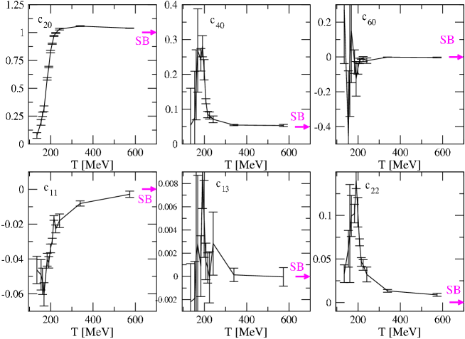
Figure 1: Some nonvanishing coefficients in the Taylor expansion of the pressure as function of the temperature along the trajectory of constant physics.

We have computed the Taylor expansion coefficients up to sixth order on the lattice ensembles along one trajectory of constant physics where we had computed the EoS at vanishing chemical potential before [3]. The trajectory is given by the choices $N_{t}=4$ and $m_{ud}\approx 0.1m_{s}$, where $m_{s}$ is tuned to the physical strange quark mass to within about 20%.

Figure 1 shows our result for some of the coefficients for the contribution to the pressure difference $\Delta p=p(\mu_{l,h}\neq 0)-p(\mu_{l,h}=0)$, see eq. (1). Note that the coefficients quickly reach the continuum Stefan-Boltzmann limit above $T_{c}$. Also note that the mixed coefficients with both $n,m\neq 0$ are quite small. Some coefficients contributing to the difference for the interaction measure $\Delta I=I(\mu_{l,h}\neq 0)-I(\mu_{l,h}=0)$ are show in figure 2.

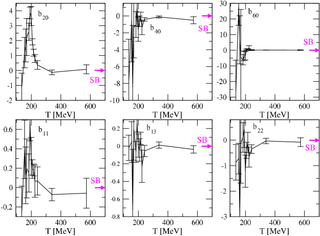
Figure 2: Some nonvanishing Taylor coefficients in the expansion of the interaction measure.

Since the pressure can be obtained by integration of the interaction measure along the trajectory of constant physics, $a^{4}p=\int_{TCP}a^{\prime 4}I(a^{\prime})d\ln a^{\prime}$, the coefficients $c_{nm}(T)$ can be obtained by integrating $b_{nm}(T)$, giving a consistency check. This is illustrated in figure 4.

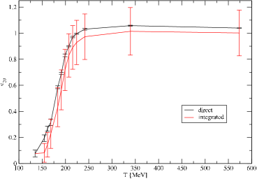
Figure 3: Comparing the two methods to compute $c_{20}(T)$, directly or by integrating $b_{20}(T)$.

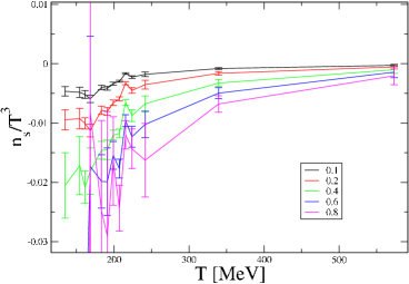
Figure 4: The induced strange quark number density $n_{s}/T^{3}$ when turning on only $\bar{\mu}_{l}/T$ and keeping $\bar{\mu}_{h}/T=0$.

Turning on $\bar{\mu}_{l}/T$ induces a small negative strange quark number density $n_{s}/T^{3}$ because some of the $c_{n1}(T)$ are nonvanishing, as shown in figure 4. To keep $n_{s}=0$, as is the case in heavy ion experiments, we need to compensate by a small tuned $\bar{\mu}_{h}/T$. We show the pressure and energy density contribution due to the nonzero chemical potential, with tuned $n_{s}=0$, in Figure 5.

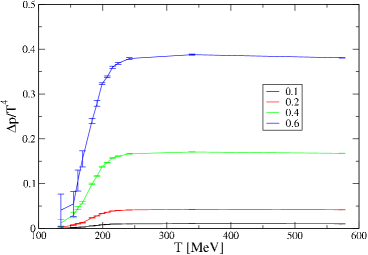
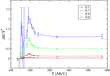
Figure 5: Pressure, $\Delta p$, and energy density, $\Delta\varepsilon$, contribution for the $m_{ud}\approx 0.1m_{s}$, $N_{t}=4$ trajectory to $O(\mu^{6})$.

4 The isentropic equation of state

Heavy ion collision experiments produce matter that, after thermalization, is expected to expand, at fixed baryon number, without further entropy generation, i.e. isentropically – with constant $s/n_{B}$. At the AGS, SPS and RHIC $s/n_{B}$ is approximately 30, 45 and 300 [6], respectively. To account for this situation, we numerically determine the $\mu_{l}$ and $\mu_{h}$, as function of $T$, by solving

$$\frac{s}{n_{B}}(\mu_{l},\mu_{h})=C,\qquad\frac{n_{s}}{T^{3}}(\mu_{l},\mu_{h})=0,$$ (8)

for $C=30$, 40, and 300, within our statistical errors. With the determined $\mu_{l}$ and $\mu_{h}$ we can then compute the isentropic equation of state, shown in figures 6 and 7 (left). For comparison, we also include the results with $\mu_{l}=\mu_{h}=0$, i.e. $s/n_{B}=\infty$.

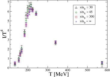
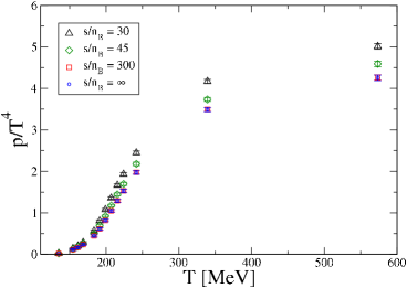
Figure 6: Isentropic versions of the interaction measure (left) and pressure (right).

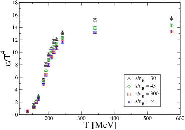
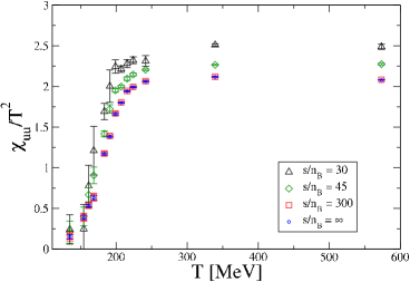
Figure 7: The isentropic energy density (left) and light-light quark number susceptibility (right).

In figure 7 (right) we show, as a further example, the isentropic light-light quark number susceptibility, $\chi_{uu}$. We note that $\chi_{uu}$ does not develop a peak structure on any of the isentropic trajectories, as would be expected near a phase transition point. Therefore all the mentioned heavy ion experiments take place far away from a possible critical (end) point in the $\mu$ – $T$ plane of the phase diagram.

5 Conclusions

We have extended the computation of the QCD equation of state for $2+1$ flavors along a trajectory of constant physics with $m_{ud}/m_{s}\approx 0.1$ on lattice ensembles with $N_{t}=4$ to small nonzero chemical potential with the Taylor expansion method up to sixth order in the chemical potential. We tuned the strange quark chemical potential to keep the strange quark density vanishing at different values of the light quark chemical potential.

We have also determined the isentropic EoS and quark number susceptibilities for values of the ratio $s/n_{B}$ relevant for heavy ion collision experiments. We found no signs of a possible phase transition along any of the considered isentropic trajectories. Qualitatively our results are in agreement with previous two-flavor studies.

Acknowledgments

This work was supported by the US DOE and NSF. Computations were performed at CHPC (Utah), FNAL, FSU, IU, NCSA and UCSB.

References

-
[1]
K. Orginos and D. Toussaint, Phys. Rev. D 59 (1999) 014501 [hep-lat/9805009];
G. P. Lepage, Phys. Rev. D 59 (1999) 074502 [hep-lat/9809157]. - [2] K. Symanzik, Plenum, New York 1980, 313.
- [3] C. Bernard et al., Phys. Rev. D 75 (2007) 105016 [hep-lat/0611031].
-
[4]
C.R. Allton et al., Phys. Rev. D 66 (2002) 074507 [hep-lat/0204010];
R.V. Gavai and S. Gupta, Phys. Rev. D 68 (2003) 034506 [hep-lat/0303013]. - [5] C. Bernard et al., arXiv:0710.1330 [hep-lat].
- [6] S. Ejiri et al., Phys. Rev. D 73 (2006) 054506 [hep-lat/0512040].