How does gas cool in DM halos?

Abstract

In order to study the process of cooling in dark-matter (DM) halos and assess how well simple models can represent it, we run a set of radiative SPH hydrodynamical simulations of isolated halos, with gas sitting initially in hydrostatic equilibrium within Navarro-Frenk-White (NFW) potential wells. Simulations include radiative cooling and a scheme to convert high density cold gas particles into collisionless stars, neglecting any astrophysical source of energy feedback. After having assessed the numerical stability of the simulations, we compare the resulting evolution of the cooled mass with the predictions of the classical cooling model of White & Frenk and of the cooling model proposed in the morgana code of galaxy formation. We find that the classical model predicts fractions of cooled mass which, after about two central cooling times, are about one order of magnitude smaller than those found in simulations. Although this difference decreases with time, after 8 central cooling times, when simulations are stopped, the difference still amounts to a factor of 2–3. We ascribe this difference to the lack of validity of the assumption that a mass shell takes one cooling time, as computed on the initial conditions, to cool to very low temperature. Indeed, we find from simulations that cooling SPH particles take most time in traveling, at roughly constant temperature and increasing density, from their initial position to a central cooling region, where they quickly cool down to $\sim 10^{4}$ K. We show that in this case the total cooling time is shorter than that computed on the initial conditions, as a consequence of the stronger radiative losses associated to the higher density experienced by these particles. As a consequence the mass cooling flow is stronger than that predicted by the classical model.

The morgana model, which computes the cooling rate as an integral over the contribution of cooling shells and does not make assumptions on the time needed by shells to reach very low temperature, better agrees with the cooled mass fraction found in the simulations, especially at early times, when the density profile of the cooling gas is shallow. With the addition of the simple assumption that the increase of the radius of the cooling region is counteracted by a shrinking at the sound speed, the morgana model is also able to reproduce for all simulations the evolution of the cooled mass fraction to within 20–50 per cent, thereby providing a substantial improvement with respect to the classical model. Finally, we provide a very simple fitting function which accurately reproduces the cooling flow for the first $\sim 10$ central cooling times.

1 Introduction

Understanding galaxy formation is one of the most important challenges of modern cosmology. The rather stringent constraints on cosmological parameters now placed by a number of independent observations (e.g., Springel et al., 2006, for a recent review) allows us to precisely set the initial conditions from which the formation of cosmic structures has started. As a consequence, understanding the complex astrophysical processes, related to the evolution of the baryonic component, represents now the missing link toward a successful description of galaxy formation and evolution. So far, two alternative approaches have been pursued to make quantitative predictions on the observational properties of the galaxy population and their evolution in the cosmological context. The first one is based on the so-called semi-analytical models (SAMs, hereafter; e.g., Kauffmann et al. 1993; Somerville & Primack 1999; Cole et al. 2000; Menci et al. 2005; Monaco et al. 2007). In this approach, the background cosmological model predicts the hierarchical build-up of the Dark Matter (DM) halos, where gas flows in, cools and gives rise to the formation of galaxies, while the complex interplay between gas cooling, star formation, chemical enrichment and release of energy from supernova (SN) explosions and Active Galactic Nuclei (AGN) is modeled through a set of simplified or phenomenological models, which are specified by a number of free parameters. A posteriori, the values of the relevant parameters should then be constrained by comparing SAM predictions to observational data. The rather low computational cost of this approach makes it a quite flexible tool to explore the model parameter space.

The second approach is based on resorting to full hydrodynamical simulations, which include the processes of gas cooling and suitable sub-resolution recipes for star formation and feedback. The obvious advantage of this method, with respect to SAMs, is that galaxy formation can be described by following in detail the gas-dynamical processes which determine the evolution of the cosmic baryons during the shaping of the large-scale cosmic structures. However, its limitation lies in the high computational cost, which makes it difficult to explore in detail the parameter space describing the process of galaxy formation and evolution. For this reason, following galaxy formation with full hydrodynamical simulations in a cosmological environment of several tens of Mpc is a challenging task for simulations of the present generation (e.g., Nagamine et al., 2004; Nagai & Kravtsov, 2005; Romeo et al., 2005; Saro et al., 2006).

This discussion shows that SAMs and hydrodynamical simulations provide complementary approaches to the cosmological study of galaxy formation. The ability of hydrodynamical simulations of accurately following gas dynamics calls for the need of a close comparison between these two approaches, in order to test the basic assumptions of the SAMs. The best regime to perform this comparison is when one excludes the effect of all those processes, like feedback in energy and metals, whose different modeling in SAMs and simulation codes would make the comparison scarcely telling. Since gas cooling is the most basic ingredient in any model of galaxy formation (e.g., White & Frenk, 1991), an interesting comparison would be performed when cooling is the only process turned on. In this spirit Benson et al. (2001), using a hydrodynamical simulation of a cosmological box and a stripped-down version of SAM, compared the statistical properties of “galaxies” found in the two cases. They discovered that SPH simulation and SAM give similar results for the thermodynamical evolution of gas and that there is a very good agreement in terms of final fractions of hot, cold and uncollapsed gas.

Similar conclusions were reached by Helly et al. (2003) and Cattaneo et al. (2007). They improved the comparison performed by Benson et al. (2001) by giving to the down-stripped SAM the same halo merger histories extracted from the cosmological simulation. In this way they were able to compare cooling in DM halos not only statistically but on an object-by-object basis. The result was again that the two methods provide comparable “galaxy” populations. Yoshida et al. (2002) performed a similar comparison for a simulation of a single galaxy cluster, obtaining similarly good results.

While the general agreement between the two methods is encouraging, still all the above analyses generally concentrated on comparing the statistical properties of the galaxy populations. Furthermore, if one wants to test the reliability of the cooling model implemented in the SAMs, the cleanest approach would be that of turning off the complications associated to the hierarchical merging of halos, thereby allowing gas to cool in isolated halos.

The purpose of this paper is to present a detailed comparison between the predictions of cooling models, as implemented in SAMs, and results of hydrodynamical simulations in which gas is allowed to cool inside isolated halos. Our controlled numerical experiments will be run for halos having the density profile (for DM particles) of Navarro et al. (1997) (NFW hereafter), with a range of masses, concentration parameters and average densities (related to the halos’ redshift). As a baseline model for gas cooling, we consider the classical one, as originally proposed by White & Frenk (1991). In this model, the cooling radius is defined as the radius at which the cooling time equals the time elapsed since radiative cooling is turned on. As a result, the growth rate of the cooled gas mass is simply related to the growth rate of the cooling radius. This model was claimed by White & Frenk (1991) to be close the exact self-similar solutions of cooling flows presented by Bertschinger (1989). Simulation results will also be compared to another model of gas cooling, which has been recently proposed by Monaco et al. (2007) in the context of the morgana SAM, and is based on a “dynamical” definition of cooling radius. As a result of our analysis, we will show that the gas cooling rate in the simulations is initially faster than predicted by the classical cooling model. When the simulations are stopped, after about 8 central cooling times, this initial transient causes the classical cooling model to underestimate the cooled mass by an amount which can be as large as a factor of three, depending on the halo concentration, density and mass. A much better agreement with simulations is achieved by the alternative morgana model.

The plan of the paper is as follows. In section 2 we describe first the “classical” analytic model for cooling (White & Frenk, 1991), and the alternative morgana cooling model (Monaco et al., 2007). In section 3 we present numerical simulations, performed with the GADGET-2 code and in section 4 we discuss the results obtained by comparing simulations to analytical cooling models. We discuss our results in section 5 and draw our final conclusions in section 6. A more technical discussion on the differences between the classical and the morgana cooling models is provided in Appendix A, while Appendix B gives a very simple fitting formula for the cooling flows.

2 Analytic models for gas cooling

2.1 Hydrostatic equilibrium in an NFW halo

All our tests start from a spherical dark matter halo with an NFW density profile,

$$\rho(r)=\rho_{\rm crit}\frac{\delta_{c}}{(r/r_{s})(1+r/r_{s})^{2}}\,,$$ (1)

where $r_{s}$ is a scale radius, $\delta_{c}$ is a characteristic (dimensionless) density, and $\rho_{\rm crit}$ is the critical cosmic density. The gas is assumed to be in hydrostatic equilibrium. The equilibrium solution for the gas can be found (Suto et al., 1998) assuming that the baryonic fraction of the halo is negligible and the gas, with density $\rho_{g}$, temperature $T_{g}$ and pressure $P_{g}$, follows a polytropic equation of state with index $\gamma_{p}$, $P_{g}\propto\rho_{g}^{\gamma_{p}}$. The equation of hydrostatic equilibrium is:

$$\frac{dP_{g}}{dr}=-G\frac{\rho_{g}M(<r)}{r^{2}}\,.$$ (2)

Here $M(<r)$ is the halo mass within $r$ (we will call $M_{200}=M(<r_{200})$ the mass within the radius $r_{200}$ encompassing an overdensity of $200\rho_{\rm crit}$), which is given by the NFW profile. Under these assumptions the equation can be solved analytically (Komatsu & Seljak, 2001):

$$\rho_{g}(r) = \rho_{g0}\left[1-a\left(1-\frac{\ln(1+c_{\rm nfw}x)}{c_{\rm nfw}x}\right)\right]^{1/(\gamma_{p}-1)}\,;$$

$$P_{g}(r) = P_{g0}\left[1-a\left(1-\frac{\ln(1+c_{\rm nfw}x)}{c_{\rm nfw}x}\right)\right]^{\gamma_{p}/(\gamma_{p}-1)}\,;$$ (3)

$$T_{g}(r) = T_{g0}\left[1-a\left(1-\frac{\ln(1+c_{\rm nfw}x)}{c_{\rm nfw}x}\right)\right]\,.$$

Here $\rho_{g0}$, $T_{g0}$ and $P_{g0}$ are the gas density, temperature and pressure at $r=0$ and $x=r/r_{200}$. Furthermore, $c_{\rm nfw}=r_{200}/r_{s}$ is the NFW concentration parameter, while $\gamma_{p}$ is the effective polytropic index, which determines the shape of the temperature profile. The constant $a$ is defined as:

$$a=\frac{\gamma_{p}-1}{\gamma_{p}}\frac{3}{\eta_{0}}\frac{c_{\rm nfw}(1+c_{\rm nfw})}{(1+c_{\rm nfw})\ln(1+c_{\rm nfw})-c_{\rm nfw}}\,.$$ (4)

The parameter

$$\eta_{0}=\frac{3r_{200}k_{B}T_{0}}{G\mu m_{p}M_{200}}$$ (5)

carries information about the central gas temperature $T_{0}$ and the mass $M_{200}$, thereby fixing the normalization of the polytropic equation of state. In eq. (5), $k_{B}$ is the Boltzmann constant, $\mu$ is the mean molecular weight ($\simeq 0.58$ for a plasma of primordial composition), and $m_{p}$ the proton mass.

Therefore, $\rho_{g0}$ is fixed by the constraint on the total gas mass $M_{g}$ within the virial radius. Calling ${\cal I}$ the integral

$${\cal I}(\alpha)=\int_{0}^{c_{\rm nfw}}\left[1-a\left(1-\frac{\ln(1+t)}{t}\right)\right]^{\alpha}t^{2}dt$$ (6)

(where for simplicity we declare only the dependence on the $\alpha$ exponent), we have

$$\rho_{g0}=\frac{M_{g}}{4\pi r_{s}^{3}}\times\frac{1}{{\cal I}(1/(\gamma_{p}-1))}\,.$$ (7)

In this way, $\eta_{0}$ is fixed by the constraint on the total gas thermal energy $E_{g}$ within the virial radius:

$$E_{g}=\frac{6\pi k_{B}T_{g0}\rho_{g0}r_{s}^{3}}{\mu m_{p}}\times{\cal I}(\gamma_{p}/(\gamma_{p}-1))\,.$$ (8)

The solution of the two conditions must be found numerically by iteration.

2.2 The classical cooling model

Most SAMs describe the cooling of gas following the model of White & Frenk (1991). The system is assumed to be in hydrostatic equilibrium at the time $t=0$. For each mass shell at radius $r$ a cooling time can be defined as:

$$t_{\rm cool}(r):=\left|{d\ln T\over dt}\right|^{-1}=\frac{3k_{B}T_{g}(r)\mu m_{p}}{2\rho_{g}(r)\Lambda(T_{g}(r))}\,,$$ (9)

where $\Lambda$ is the cooling function. The left-hand-side of the above equation follows from the assumption that $dT$ is computed for an isobaric transformation. In the following, we assume, for both simulations and analytical models, $\Lambda(T)$ to be that tabulated by Sutherland & Dopita (1993) for zero metallicity. The cooling radius at the time $t$ for the classical model, $r_{\rm C}(t)$, is the defined through the relation

$$r_{\rm C}(t):\ \ \ t_{\rm cool}(r_{\rm C})=t\,.$$ (10)

In other words, the function $r_{\rm C}(t)$ is the inverse of the function $t_{\rm cool}(r)$. It is then assumed that each shell cools after one cooling time. The resulting mass deposition rate reads

$$\dot{M}_{\rm cool}=4\pi r^{2}\rho_{g}(r_{\rm C})\frac{dr_{\rm C}}{dt}\,.$$ (11)

where a dot denotes a time derivative.

We emphasize that the classical cooling model imposes that a shell of gas cools exactly after one cooling time, computed on the initial configuration. The mass cooling rate of equation (11), predicted by this model, is generally not far from that of the self-similar solutions of cooling flows found by Bertschinger (1989). This point will be further discussed in Section 5 and in the Appendix.

2.3 The morgana cooling models

In the classical cooling model, hot gas is assumed to be located outside the cooling radius $r_{\rm C}$. This same assumption is used in the morgana cooling model; we call this cooling radius $r_{\rm M}$ to distinguish it from the classical one. The equilibrium gas configuration is computed as in equations (3), but taking into account that no hot mass is present within $r_{\rm M}$; this implies that the integral in equation (6) is evaluated from $r_{\rm M}/r_{s}$ to $c_{\rm nfw}$.

Given the equilibrium profile, the cooling rate of a shell of gas of width $\Delta r$ at a radius $r$ is:

$$\Delta\dot{M}_{\rm cool}(r)=\frac{4\pi r^{2}\rho_{g}(r)\Delta r}{t_{\rm cool}(r)}\,,$$ (12)

where $t_{\rm cool}$ is given by equation (9). The mass deposition rate is then computed by integrating the contributions of all the mass shells. In performing this integral, we note that the cooling time depends on density and temperature, the density dependence being always stronger since the temperature profile is much shallower than the density profile. The integration in $r$ can then be performed by assuming $T_{g}(r)\simeq T_{g}(r_{\rm M})$, while taking into full account the radial dependence of the density. The resulting total mass deposition rate can then be written as

$$\dot{M}_{\rm cool}=$$

$$\frac{4\pi r_{s}^{3}\rho_{g0}}{t_{\rm cool,0}}\int_{r_{\rm M}/r_{s}}^{c_{\rm nfw}}\left[1-a\left(1-\frac{\ln(1+t)}{t}\right)\right]^{2/(\gamma_{p}-1)}t^{2}dt.$$

We apply this mass cooling rate starting from $t=t_{\rm cool}(0)$ (the cooling time at $r=0$), under the hypothesis that nothing cools before that time. The rate of thermal energy loss by cooling is computed in a similar way:

$$\dot{E}_{\rm cool}=\frac{3kT_{g}(r_{\rm cool})}{2\mu m_{p}}\frac{4\pi r_{s}^{3}\rho_{g0}}{t_{\rm cool,0}}$$

$$\times\int_{r_{\rm M}/r_{s}}^{c_{\rm nfw}}\left[1-a\left(1-\frac{\ln(1+t)}{t}\right)\right]^{2/(\gamma_{p}-1)}t^{2}dt\,.$$

The lower extreme of integration comes from the assumption that the hot and cold phases are always separated by a sharp transition, taking place at the cooling radius $r_{\rm M}$. By equating the mass cooled in a time interval $dt$ with the mass contained in a shell $dr$, one obtains the evolution of the cooling radius:

$$\dot{r}_{\rm M}=\frac{\dot{M}_{\rm cool}}{4\pi\rho_{g}(r_{\rm M})r_{\rm M}^{2}}\,.$$ (15)

The evolution of the system is then followed by numerically integrating the equations (2.3), (2.3) and (15), starting after a time $t_{\rm cool}(0)$. The integration is performed with a simple Runge-Kutta integrator with adaptive time-step and the gas profile is re-computed at each time step. Clearly, as long as the mass and thermal energy of each cooled shell is removed from the profile, the rest of the gas is unperturbed so its profile does not change with time.

The two main assumptions at the base of the morgana cooling model are: (i) all mass shells contribute to cooling according to equation (12), (ii) there is anyway a sharp transition from the hot to the cold phase, which guarantees the presence of a sharp border separating the regions where cooled and hot gas resides.

Equation (15) is valid under the assumption that the gas is pressure-supported at the cooling radius, which is clearly false in general. In particular, as long as the time derivative of the cooling radius is much larger than the gas sound speed, the boundary of the cooled region propagates so quickly that any gas motion can be neglected. This holds only at early times and, therefore, for very low $r_{\rm M}$ values. On the contrary, the late evolution of cooling is better represented by letting the “cooling hole” close at the sound speed. We then define a further cooling radius $r_{\rm M,ch}$, whose evolution is given by the equation:

$$\dot{r}_{\rm M,ch}=\frac{\dot{M}_{\rm cool}}{4\pi\rho_{g}(r_{\rm M,ch})r_{\rm M,ch}^{2}}-c_{s}(r_{\rm M,ch})\,.$$ (16)

Here $c_{s}$ is the sound speed evaluated at the cooling radius. This simple change strongly influences the predictions of the cooling model. In fact, the evolution of the cooling radius turns out to be remarkably different, with $r_{\rm M,ch}<r_{\rm M}$; as a consequence, because the gas profile is recomputed at each time-step, the mass re-distributes over the available volume, at variance with the previous case in which the gas profile remains unperturbed beyond $r_{\rm M}$. We will refer to the models of equations (15) and (16) as the “unclosed” and “closed” morgana cooling models, respectively.

Equation (16) clearly gives an oversimplified description of the process in play, with the implicit assumption that the gas has time to settle into a new hydrostatic equilibrium configuration. However, due to the negative gas temperature profile, the uncooled gas is predicted to become progressively colder, with the result that the density and temperature profiles become steeper to keep satisfying the condition of hydrostatic equilibrium. Eventually, this leads to a catastrophic cooling involving all the the gas of the halo. A simple and effective way to obtain an acceptable behaviour for $M_{\rm cool}$ is to suppress the sound speed term of equation (16) when the specific thermal energy of the hot gas becomes smaller than the specific virial energy ($-0.5\,U_{H}/M_{H}$, where $U_{H}$ is the binding energy of the DM halo). Since this is admittedly an ad-hoc solution to the above problem, our attitude is to consider the “closed” morgana model as an effective model to describe the evolution of the cooled mass in DM halos.

In summary, we have identified three analytic cooling models: classical, unclosed morgana and closed morgana. The main difference between the classical and unclosed morgana model is the following: while the classical model equates the time required for a shell to cool to low temperature with the cooling time computed on the initial conditions (eq. 9), the unclosed morgana model does not rely on this strong assumption. The main difference between the unclosed and closed morgana models is that the latter attempts a more realistic description of the evolution of the cooling radius, taking into account that the cooled gas cannot provide pressure support to the inflowing cooling gas.

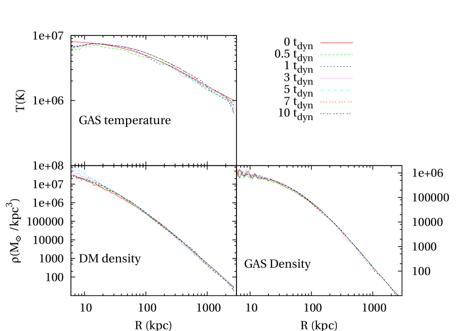
Figure 1: Profiles of gas temperature (Top panel), DM density (Bottom left panels) and gas density (Bottom right panel) for the non-radiative run of the halo H1, evaluated at 7 different epochs in the interval $[0,10]t_{dyn}$.

3 The simulations

The simulations that we will discuss in this paper have been obtained by evolving initial conditions for gas sitting in hydrostatic equilibrium within isolated halos whose DM density profile is the NFW one. They have been performed using GADGET-2 code, a massively parallel Tree+SPH code (Springel, 2005) with fully adaptive time-step integration. The version of the code that we used adopts an SPH formulation with entropy conserving integration and arithmetic symmetrization of the hydrodynamical forces (Springel & Hernquist, 2002), and includes radiative cooling computed for a primordial plasma with vanishing metallicity. The above SPH formulation is also that used by Yoshida et al. (2002) in their comparison between SAMs and hydrodynamical simulations. It ensures the suppression of spurious cooling at the interfaces between cooled and hot gas (see also Tornatore et al., 2003). In order to follow in detail the trajectories of gas particles in the phase diagram, while they are undergoing cooling, we have implemented a quite conservative criterion of time-stepping, in which the maximum time-step allowed for a gas particle is one tenth of its cooling time.

In the following, we will present simulations based on including radiative cooling along with a simple recipe for star formation, but excluding any form of energy feedback from supernovae. Only in one case, in which we want to study the structure and the evolution of the phase diagrams, we turned star formation off. The star formation recipe adopted assumes that a collisional gas particle, whose equivalent hydrogen number density exceeds $n_{H}=0.1$ cm^-3 and with temperature below $3\times 10^{4}$K, is instantaneously converted into a collisionless “star” particle. The practical advantage of including star formation is that the simulations becomes computationally much faster, since one avoids performing intensive SPH computations among cooled high-density gas particles. As we shall discuss in the Section 4, we verified that the evolution of the mass deposition rate is essentially independent of the introduction of star formation.

Initial conditions for isolated halos have been created by placing gas in hydrostatic equilibrium within a DM halo, having the NFW density profile (see eq. 1), according to the model given in section 2.1. To fix the gas thermal energy, we required, as suggested by Komatsu & Seljak (2001), that the slopes of the DM and gas density profiles be equal at the virial radius. This leads to thermal energies very similar to 1.2 times the virial energy, as used by Monaco et al. (2007). In order to generate initial conditions, initial positions of DM and gas particles are generated by Monte Carlo sampling the analytical profiles of eqs. (1) and (3). To create an equilibrium configuration for the DM halo, initial velocities of the particles are assigned according to a local Maxwellian approximation (Hernquist, 1993), where the width of the distribution is given by the velocity dispersion of the DM particles, as obtained by solving the Jeans’ equation. As for the gas particles, their internal energy is assigned according to the third of the equations (3). Since the above equations are a hydrostatic solution, gas particles are initially assigned zero velocities.

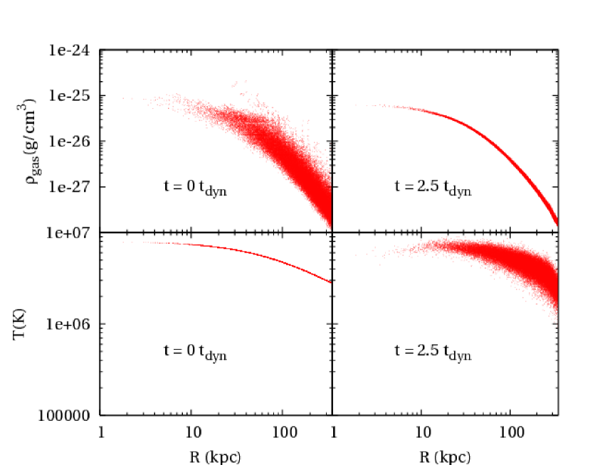
Figure 2: Top panels: Density of gas particles for the non-radiative run of the halo H1, as a function of their halo-centric distance, at $t=0$, as assigned in the initial conditions (left) and after $2.5t_{\rm dyn}$ (right). Bottom panels: the same as for the top panels, but for the temperature of gas particles.

Table 1: Characteristics of the simulated halos. Column 1: halo name; column 2: halo mass enclosed within $r_{200}$; Column 3: NFW concentration parameter; Column 4: redshift used to compute the reference critical density; Column 5: value of $r_{200}$ (in kpc); Columns 6: dynamical time (in Gyr); Column 7: central cooling time (in Gyr).

	$M_{200}$	$c_{\rm nfw}$	redshift	$r_{200}$	$t_{\rm dyn}$	$t_{\rm cool,0}$
$H1$	$10^{13}$	$6.3$	$z=0$	$350$	$0.56$	$0.56$
$H2$	$10^{13}$	$7.25$	$z=0$	$350$	$0.56$	$0.40$
$H3$	$10^{13}$	$5.25$	$z=0$	$350$	$0.56$	$0.82$
$H4$	$10^{12}$	$7.25$	$z=0$	$162$	$0.56$	$0.12$
$H5$	$10^{15}$	$4.3$	$z=0$	$1623$	$0.56$	$6.67$
$H6$	$3\cdot 10^{11}$	$6.53$	$z=1$	$75$	$0.32$	$0.04$
$H7$	$10^{13}$	$5.63$	$z=1$	$241$	$0.33$	$0.31$
$H8$	$10^{12}$	$5.92$	$z=2$	$79$	$0.19$	$0.04$

Each halo has been sampled with $6\times 10^{4}$ DM particles inside $r_{200}$ and an initially equal number of gas particles. The ratio between the mass of DM and gas particles is determined by the baryon fraction, that we assume to be $f_{\rm bar}=0.19$. As for the choice of the gravitational softening, it has been chosen to be about three times larger than the lower limit recommended by Power et al. (2003), $\epsilon\simeq 3r_{200}/\sqrt{N_{200}}$ for a Plummer-equivalent softening, where $N_{200}$ is the number of particles within $r_{200}$. The minimum value allowed for the SPH smoothing length is assumed to be 0.5 times the value of the gravitational softening, with SPH computations performed using $N_{\rm ngb}=32$ for the number of neighbours.

To ensure stability of the halos in the absence of cooling, density profiles have been sampled with particles out to about $8r_{200}$. This also ensures an adequate reservoir of external gas than can flow in while cooling removes pressure support in the central halo regions. In principle, our controlled numerical experiments could have been performed by using a static NFW potential, instead of sampling the halo with DM particles. However, this procedure would not have allowed us to account for any backreaction of cooling on the DM component. Indeed, it is known from cosmological simulations that including gas cooling causes a sizeable change (adiabatic contraction) of the structure of the DM halos (e.g., Gnedin et al., 2004).

The characteristics of the simulated halos are summarized in Table 1. In this table we also specify the redshift at which the simulated halo is assumed to stay. Although redshift never explicitly enters in our simulations of isolated halos, it appears in a indirect way when we fix the value of the critical density. Ultimately, increasing redshift amounts to take a higher value of $\rho_{\rm crit}$ and, therefore, a higher halo density for a fixed value of $M_{200}$. In this way, we expect that “high-redshift” halos will have a shorter cooling time. In the following, we assume the relation between redshift and critical density to be that of a cosmological model with $\Omega_{m}=0.3$ and $\Omega_{\Lambda}=0.7$.

Our reference halo has a mass $M_{200}=10^{13}M_{\odot}$ (H1 in Table 1), typical of a poor galaxy group, with a value of the concentration parameter $c_{\rm nfw}=6.3$, given by the relation between mass and concentration provided by NFW, and $r_{200}$ corresponding to the value of $\rho_{\rm crit}$ at $z=0$. Two other halos of the same mass are also simulated, which have different values of the concentration parameter, still lying within the scatter in the $M_{200}$–$c_{\rm nfw}$ relation (H2 and H3). We then simulate a smaller (H4) and a larger (H5) halo, with $M_{200}=10^{12}M_{\odot}$ and $M_{200}=10^{15}M_{\odot}$, respectively, so as to sample also the scale of elliptical galaxies and of rich clusters. We finally consider two halos at $z=1$ (H6 and H7) and one halo at $z=2$ (H8). In all runs we used the same value, $\gamma_{p}=1.18$, for the effective polytropic index. In Table 1 we also report for each halo the values of the dynamical time-scale, which is defined as

$$t_{\rm dyn}=\Bigg{(}\frac{1}{4\pi G\rho}\Bigg{)}^{1/2}\,,$$ (17)

and that of the cooling time calculated at the center of the halo as in equation (9).

In order to verify the numerical stability of our results, we also performed the following runs for the H1 halo: (a) a simulation with a 10 times larger number of particles and a rescaling of the softening, in order to check the effect of mass resolution (H1-HR); (b) a simulation with a 4 times larger number of particles (at fixed halo mass) and number of neighbours $N_{\rm ngb}$ than in the reference run, keeping the softening constant for the gravitational force (H1-4SPH): because mass resolution is given by $N_{\rm ngb}$ times particle mass, this is kept constant while decreasing the discreteness noise in the SPH computation; (c) a simulation with cooling only and without star formation (H1-C); (d) a simulation in which the gravitational softening is halved with respect to the reference value (H1-S).

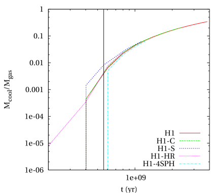
Figure 3: Evolution of the cooled mass $M_{\rm cool}$ for different runs of the H1 halo. Solid line: reference run with cooling and star formation; dashed curve: run with only cooling (H1-C); short-dashed curve: run with cooling and star formation, with halved gravitational softening (H1-S); dotted curve: run with cooling and star formation at 10 times better mass resolution (H1-HR); dotted-dashed curve: run with cooling and star formation at 4 times more particles and SPH neighbours (H1-4SPH) . The vertical black line represents the theoretical central cooling time.

All the initial conditions have been first evolved for 10 dynamical times, without cooling. This allowed us to check that temperature and density profiles are always stable, thus confirming that the initial conditions are indeed quite close to configurations of hydrostatic equilibrium. An example of this is shown in Figure 1, where we plot the profiles of gas density, DM density and temperature for the reference halo H1, at different epochs. Although the profiles are all remarkably stable, it is worth reminding that there are at least two reasons why our initial conditions may not be equilibrium configurations. Firstly, the gas profiles given by equations (3) are not an exact equilibrium solution because the gas mass is not negligible. Secondly, initial particle positions are assigned by performing a Monte Carlo sampling of the gas and DM density profiles, while the internal energy of gas particles is assigned in a deterministic way, by using the third of the equations (3). The scatter associated to the Poissonian sampling of the density profiles, joined with the deterministic assignment of the internal energy of SPH particles, may well not represent a configuration of stable equilibrium. If this is the case, we then expect that the system relaxes to the true minimum energy configuration in a time comparable to its dynamical time-scale. Indeed, Figure 2 shows the scatter plot of individual values of density and temperature of all the gas particles, as a function of their halo-centric distance, for the initial conditions of H1 (left panels) and for a configuration obtained by evolving the system for $2.5t_{\rm dyn}$ in the absence of cooling (right panels). The relaxed configuration shows residual scatter both in density (amounting to 5 per cent) and temperature (amounting to 15 per cent). The same amount of scatter is also found in the high resolution run (H1-HR), while a smaller amount (3 per cent in density, 5 per cent in temperature) is found in the H1-4SPH simulation, where the density is computed averaging over 128 instead of 32 particles. The latter result suggests a numerical origin for this scatter, related to the finite number of particles used in the SPH computations.

In order to account for this relaxation, we decided to use as initial conditions for the radiative runs the configuration attained by evolving the non-radiative runs for $2.5$ dynamical times. Once cooling is turned on, all simulations are let then evolving for 8 central cooling times, with the exception of H5, which is run for roughly two central cooling times.

4 Results

As already emphasized, the main aim of our analysis is to understand the radiative cooling of the gas in DM halos and to point out which one of the cooling models, described in section 2, gives results on the evolution of the cooled gas mass which are in best agreement with the numerical experiment. To this purpose, most of the discussion on how gas cools in simulations will refer to the H1 halo. Since the evolution of $M_{\rm cool}$ is the central result of our analysis, we will show it for all the halos and compare the simulation results with the predictions of the cooling models.

In Figure 3 we show the evolution of $M_{\rm cool}$ for the reference run of the halo H1 (i.e. cooling and star formation), and compare it with the same run without star formation (H1-C), with the run having 10 times better mass resolution (H1-HR), four times more particles and SPH neighbours (H1-4SPH) and with the run with standard mass resolution but with gravitational softening smaller by a factor of two (H1-S). In the runs with cooling and star formation, $M_{\rm cool}$ is contributed both by the mass in collisionless stars and by the mass in cold gas particles, which have temperature below $3\times 10^{4}$ K. In the run with cooling only, $M_{\rm cool}$ is clearly contributed only by particles colder than the above temperature limit. Figure 3 shows that the evolution of the cooled mass is independent of whether cold and dense particles are treated as collisionless or SPH particles. This result, which agrees with that found by Tornatore et al. (2003) for cosmological simulations of clusters, confirms that using the SPH scheme with explicit entropy conservation and arithmetic symmetrization of hydrodynamical forces Springel & Hernquist (2002) is able to suppress the spurious gas cooling which otherwise takes place at the interface between cold and hot phases. This result also demonstrates that including star formation in the radiative runs does not affect our results on $M_{\rm cool}$. As for the run with a larger number of neighbours (H1-4SPH), cooling turns out to start at a later epoch. The reason for this lies in the reduced scatter in density in the initial conditions, when a larger number of neighbours for the SPH computations is used. In fact, a gas particle whose density is scattered upwards with respect to the density computed from the profile at its halo-centric distance, has a shorter cooling time. As a consequence, the smaller the scatter, the lower the probability that a gas particle has cooling time significantly shorter than that relative to its radial coordinate. As for the high-resolution run (H1-HR), the larger number of particles provides a better sampling of the scattered density distribution. Therefore, there is an increasing probability to have a small number of gas particles, with exceptionally up-scattered density, which cool down at earlier times. Finally, decreasing the gravitational softening by a factor 2 (H1-S run) leads to better resolving the very central part of the halo, where gas can more easily cool. This turns into a stronger initial transient in the evolution of $M_{\rm cool}$ at the onset of cooling. Quite reassuringly, despite the differences in the evolution of $M_{\rm cool}$ between these runs during the first cooling time, they all nicely converge after about two cooling times. This demonstrates that our numerical description of the evolution of the cooled mass is numerically stable after an initial transient.

In order to probe in detail the behaviour of gas in radiative simulations, we have randomly selected five particles in three distance intervals from the center (10-20 kpc, 30-40 kpc and 50-60 kpc) in the initial conditions and we have followed their evolution in the H1-C run (the absence of star formation allows to follow the transition from the hot to the cold phase). In Figure 4 we plot the evolution of temperature and density as a function of time for the selected particles.

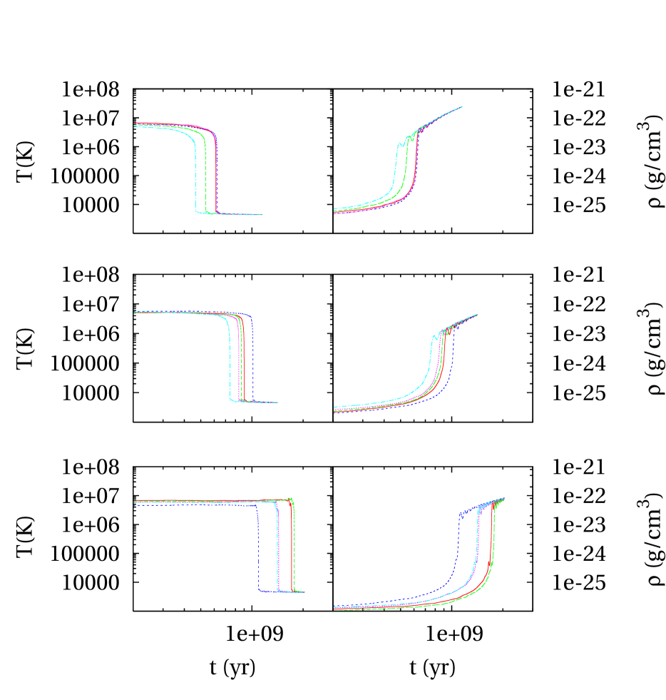
Figure 4: Evolution of temperature (left panels) and density (right panels) for three sets of five particles each, selected within three different radial shells in the initial conditions. Top panels: $(r_{\rm min},r_{\rm max})=(10,20)$ kpc; Central panels:$(r_{\rm min},r_{\rm max})=(30,40)$ kpc. Bottom panels: $(r_{\rm min},r_{\rm max})=(50,60)$ kpc.

While flowing toward the halo centre, each particle roughly maintains its initial temperature while its density progressively increases. Afterwards, in a very short time interval, it cools down to $\raise-2.0pt\hbox{\hbox to0.0pt{\hbox{$\sim$}\hss}\raise 5.0pt\hbox{$<$}\ }10^{4}$K, which corresponds to the temperature where the cooling function dies. This means that the transition from the hot to the cold phase takes place quite rapidly, thus keeping the two phases well separated.

Figure 5 shows the scatter plot of temperature vs. halo-centric distance of the gas particles in the H1-C run at two output times. It is possible to identify a “cooling region” as the spherical shell where the drop in temperature takes place. It is interesting to note that the size of this region is roughly constant in time and comparable to the softening scale. We have verified that the presence of a sharp physical boundary separating hot and cold gas phases is robust against numerical resolution, in fact with an even sharper boundary at higher resolution, but its size does depend on resolution. In the H1-HR run, who has roughly a two times smaller softening, the size of the cooling region is more than 50 per cent smaller. Therefore, while our simulations provide a numerically convergent result on the evolution of $M_{\rm cool}$, they do not provide a similarly convergent result on the size of the cooling region.

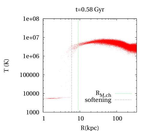
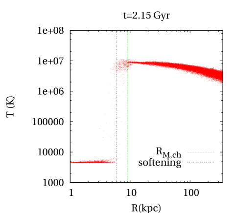
Figure 5: Scatter-plot of temperature vs. halo-centric distance for gas particles in the run of the H1 halo which includes only cooling, without star formation (H1-C). The green, dotted lines give the cooling radius $r_{\rm M,ch}$ as predicted by the closed morgana model, while the black, dashed lines denote the softening scale.

In Figure 6 we show the density profile of DM and the density, pressure and temperature profiles of the hot gas in the simulation at several times, normalized to the corresponding profiles evaluated for the initial conditions. Pressure increases in the inner part of the halo for a few dynamical times, to saturate later to values that peak at a factor of six times higher than in the initial conditions, just outside the cooling region. This increase in pressure is mainly driven by a comparable increase in gas density, while the temperature profile is much more stable or even slightly decreasing near the cooling region. The density increase on the other hand is partly caused by the adiabatic contraction of the DM halo, but because the increase in DM density, though significant, is smaller than that in gas density, then adiabatic contraction gives only a minor contribution. As we shall discuss in the following, the increase in gas density enhances radiative losses as the gas approaches the cooling region, and this turns into a shortening the cooling time of the inflowing gas particles, with respect to the predictions of the classical model.

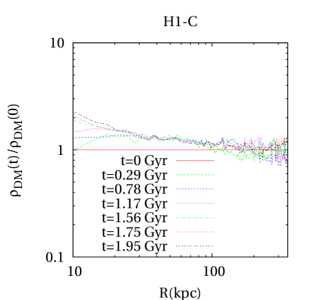
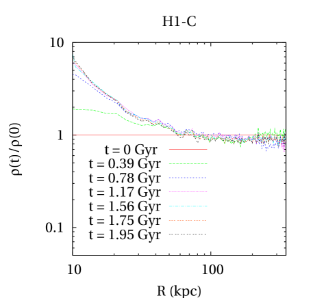
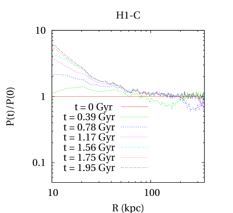
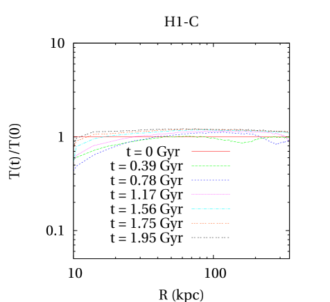
Figure 6: Profiles of DM density (upper left panel), gas density (upper right), pressure (lower left) and temperature (lower right) at different epochs for the H1 simulation with only cooling (H1-C). All profiles are normalized to their initial value.

In summary, the following conclusions can be drawn from our analysis of gas cooling in simulations:
(i) the drop in temperature when gas particles pass from the hot to the cold phase is quite rapid;
(ii) this drop in temperature takes place in a spherical shell with a rather sharp boundary, the cooling region, which separates the inner and outer regions dominated by cold and hot particles, respectively;
(iii) density and pressure increase with time just beyond the cooling region, and this increase is not driven by adiabatic contraction of the halo.

In the light of these results, the question then arises as to whether the cooling recipes, described in section 2, able to reproduce the rate of mass cooling found in the simulations.

In order to answer this question, we first address the issue concerning the tuning of the initial conditions. As mentioned in section 3, the gas in the simulations relaxes to a minimum energy configuration, so that the parameters of the gas profile after 2.5 dynamical times, when the cooling is turned on, may in principle differ from the ones used to generate the initial conditions. This is a crucial point because in order to make a reliable comparison between analytic cooling models and numerical simulations, we must be sure that the initial conditions are the same for both. Owing to the stability of the profiles shown in Figure 1, we expect this effect to be small. As we shall see, even small differences in the initial profiles leads to an appreciable change in the resulting evolution of $M_{\rm cool}$. In the model that we used to generate the initial hydrostatic configurations (equations 3), the parameters that determine the gas density and the temperature profiles are the halo gas mass $M_{g}$, the effective polytropic index $\gamma_{p}$, and the central temperature of the gas (in units of the virial one) $\eta$. While holding the mass fixed, we have considered 900 pairs of values for the parameters $(\gamma_{p},\eta)$, varying both the polytropic index and the energy factor in the range $[1.1:1.4]$. We have calculated for each pair the theoretical density and temperature profiles according to equations (3), and compared them with the profiles from the initial conditions. In particular, we calculated for each radius the root mean square difference between the density and temperature profiles of the hydrostatic model and those of the initial conditions, and imposed the maximum difference to be smaller than 10 per cent. Then, for each cooling model and unless otherwise stated, we show predictions relative to all the profiles that were selected by the procedure described above. This allows us to keep control on any uncertainty of the initial profiles which are used as input to the cooling models.

As a main term of comparison between analytic models and simulations, we use the evolution of the cooled mass fraction. In Figure 7 we plot the evolution of $M_{\rm cool}$ for all the eight simulated halos from simulations and the predictions of the different cooling models. As for the latter, each shaded area represent the envelope of each model prediction for all the profiles which provide a good fit to the initial conditions.

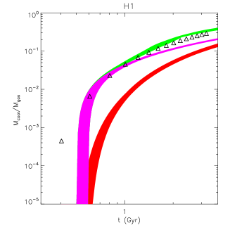
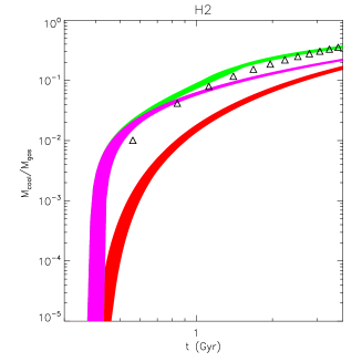
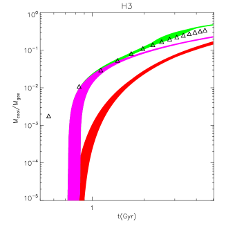
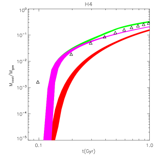
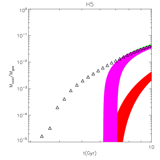
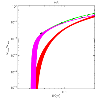
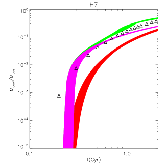
Figure 7: Evolution of the cooled gas fraction, $M_{\rm cool}$, for the eight simulated halos, in the radiative runs with star formation. Open triangles are the simulation results, while the shaded areas (in color in the online version) represent the prediction of the three different models. Classical model: darkest shade, red; unclosed morgana: lightest shade, magenta; closed morgana: middle shade, green). Each area represents the envelopes of hydrostatic models which provide a good fit to the initial conditions (see text).

From these plots we infer the following conclusions.

(i) No gas is allowed to cool down to low temperatures before one central cooling time has elapsed, both in the classical and in the morgana models. Afterwards, cooling takes place abruptly, giving rise to a sort of “burst” of star formation. This behaviour is consistent with simulation results, at least when the scatter in density and temperature, which are present in the initial conditions, is reduced.
(ii) The classical cooling model (red area) always underpredicts the value of $M_{\rm cool}$. This underestimate is more severe at earlier times, and remains quite substantial, a factor of 2–3, even in the most evolved configurations. This effect is generally stronger for the halos having a lower concentration and/or higher mass, i.e. having longer cooling times (see Table 1).
(iii) The unclosed morgana model (magenta area) follows in a much closer way the cooled mass at early times and the fit is very good in most cases at epochs between one and a few central cooling times. In the most evolved configurations, the model underestimate the cooled mass, although the underestimate is sensibly reduced with respect to the classical model.
(iv) The closed morgana model behaves very similarly to the unclosed one for a few central cooling times. At later times, it predicts a larger value of $M_{\rm cool}$, providing a generally good fit to the simulation results for the most evolved configurations.

5 Discussion

The better performance of the unclosed morgana model, with respect to the classical model, in reproducing the evolution of the cooled gas fraction from the simulations can be ascribed to the following facts.

As explained in Section 2.4, the classical model relies on the strong hypothesis that each gas shell cools in exactly one cooling time, with this cooling time computed on the initial conditions. While this hypothesis is valid when the first gas particles cool, it breaks down soon later. This behaviour is indeed not unexpected. The evolution of a mass element in presence of cooling and adiabatic compression is given by the following equation:

$$\dot{T}=T\left(-\frac{1}{t_{\rm cool}}+\frac{2}{3}\frac{\dot{\rho}}{\rho}\right)\,,$$ (18)

where $\rho(t)$ and $T(t)$ describe the evolution of density and temperature of the gas element, and $t_{\rm cool}$ is the cooling time computed on the actual density and temperature (not on the initial conditions). Under the assumptions that the temperature dependence of the cooling time can be neglected, so that $t_{\rm cool}(t)=t_{\rm c0}(\rho(t)/\rho_{0})^{-1}$, and that pressure is constant during the evolution, it is easy to solve equation (18) and find that the time $t_{\rm tot}$ required for the mass element to cool to $T=0$ coincides with $t_{\rm c0}$. Therefore, the basic assumption of the classical model is satisfied in the case in which gas particles cool at constant pressure.

On the other hand, Figure 4 shows that gas particles take most time to flow from their initial position to the cooling region. Since cooling takes place in a pressure-supported way during this time, their radiative losses are balanced by adiabatic compression. As a result, the temperature of the gas particles has a slow evolution while density increases significantly as they move towards the cooling region. This results in shallow and stable temperature profiles, while density profiles become progressively steeper (see Figure 6). The density increase turns into enhanced radiative losses, thereby making the total cooling time, $t_{\rm tot}$, shorter than the cooling time, $t_{\rm c0}$, computed on the initial conditions.

The main assumption of the classical model is then clearly invalidated by our simulations. Going back to the original proposal of this model by White & Frenk (1991), the main justification was that the model is roughly consistent with the exact self-similar solutions found by Bertschinger (1989). However, Bertschinger’s self similar solutions give cooling flows that are equal to:

$$\dot{M}_{\rm cool}=4\pi r^{2}\rho_{g}(r_{\rm C})\frac{dr_{\rm C}}{dt}\times\mu_{0}\,,$$ (19)

where the constant $\mu_{0}$ depends on the initial profile and can take values ranging from $\sim 0.1$ to $\sim 2.5$ (see tables 1 and 2 in Bertchinger’s paper). The classical model is recovered in the case $\mu_{0}=1$. In the Appendix we will consider the simple case of an isothermal halo with power-law density profile $\rho_{g}\propto r^{-2}$. In this case the unclosed morgana model gives $t_{\rm tot}=0.5t_{\rm c0}$ and a mass-deposition rate, $\dot{M}_{\rm cool}$, which is equal to $\sqrt{2}$ times that of the classical model. On the other hand, Bertschinger’s solutions give cooling flows higher than the classical value by a factor ranging from 1.304 to 1.190, depending on the shape of the cooling function, thus implying total cooling times $t_{\rm tot}$ shorter than $t_{\rm c0}$ by a factors ranging from 0.59 to 0.70. Both morgana and Bertschinger’s self-similar solutions predict that shallower power-law profiles give stronger cooling flows and shorter total cooling times. Therefore, while the unclosed morgana model agrees with the exact self-similar solution to within a few tens per cent, the assumption that $t_{\rm tot}=t_{\rm c0}$ is generally not correct.

More in detail, the difference between classical and unclosed morgana models at the onset of cooling is the consequence of the flatness of the density profile in the inner regions of the gas. This can be shown by finding exact solutions of the classical and morgana models in the case of power-law density profiles, $\rho_{g}(r)\propto r^{-\alpha}$, for an isothermal gas. These calculations are reported in the Appendix and the results can be summarized as follows. (i) Both the unclosed morgana model and the classical one predict a self-similar cooling flow for $\alpha>3/2$, thus implying that the corresponding mass deposition rates are proportional to each other. (ii) The classical and unclosed morgana models agree if $\alpha=3$; shallower profiles lead the unclosed morgana model to predict shorter total cooling times and higher cooling rates. (iii) For profiles flatter than $\alpha=3/2$ the mass cooling flow of the unclosed morgana model is dominated by the external regions. The solution is not proportional to the classical one, the cooling flow is not self-similar and is roughly constant. Clearly, such a shallow profile will hold in the inner region of a realistic halo.

As a conclusion, the strict validity of the classical model is limited to specific profiles and to self-similar flows. On the other hand, the unclosed morgana model, which relaxes the assumption on the total cooling time of a gas shell, better reproduces the stronger flows found in our simulations of isolated halos, which takes place when the Lagrangian cooling radius sweeps the flat part of the density profile.

The closed morgana model further improves the agreement with the simulations by increasing the fraction of cooled mass. The main reason for this increase is that, being always $r_{\rm M,ch}<r_{\rm M}$, the smaller value of the cooling radius leads to an increase of the density of the cooling shell, simply because the hot gas is allowed to stay at smaller radii. This implies still shorter cooling times and enhanced cooling flows. Another prediction of the closed morgana model is that the cooling radius $r_{\rm M,ch}$ is stable after a quick transient. This prediction is in qualitative agreement with the results of the simulations (see Figure 5; the dotted lines give the position of $r_{\rm M,ch}$). However, the size of the cooling region in the simulation is affected by resolution, so this comparison cannot be pushed to a quantitative level. The validity of this model breaks as soon as the energy of the uncooled gas drops below the virial value. In this case we still obtain a good match of the cooled mass fraction by simply dropping the sound speed term in equation (16), which is responsible for the shrinking of the cooling hole. For this reason, we consider the closed morgana model as an effective model, in that it takes into account the shrinking of the cooling region caused by the pressure from the hot gas just outside this region, without however providing a formally rigorous description for this effect.

Using the predicted rough constancy of the cooling flow when the central, shallow part of the gas profile is cooling, in Appendix B we show that it is possible to give a very simple and remarkably accurate prediction of the cooled mass as the result of a constant flow which is given by a simple analytic formula, valid up to $\sim 10$ central cooling times.

6 Conclusions

We have presented a detailed analysis of cooling of hot gas in DM halos, comparing the predictions of semi-analytic models with the results of controlled numerical experiments of isolated NFW halos with hot gas in hydrostatic equilibrium. Simulations have been performed spanning a range of masses (from galaxy- to cluster-sized halos), concentrations and redshift (from 0 to 2). Smaller halos at higher redshift have not been simulated because the validity of the assumption of a hydrostatic atmosphere is doubtful when the cooling time is much shorter than the dynamical time.

We have considered the “classical” cooling model of White & Frenk (1991), used in most SAMs, and the model recently proposed by Monaco et al. (2007) within the morgana code for the evolution of galaxies and AGNs. The main features of these models can be summarized as follows. The density and pressure profiles of the gas are computed by solving the equation of hydrostatic equilibrium in an NFW halo (Suto et al., 1998). The classical cooling model assumes that each mass shell cools to low temperature exactly after one cooling time $t_{\rm cool}(r)$, computed on the initial conditions. The cooling radius $r_{\rm C}$ is then the inverse of the $t_{\rm cool}(r)$ function, and the cooled fraction is the fraction of gas mass within $r_{\rm C}$. The “unclosed morgana” cooling model computes the cooling rate of each mass shell, then integrates over the contribution of all mass shells and follows the evolution of the cooling radius assuming that the transition from hot to cold phases is quick enough so that a sharp border in the density profile of hot gas is always present. This determines the evolution of the cooling radius $r_{\rm M}$. Moreover, to mimic the closure of the “cooling hole” due to the lack of pressure support at $r_{\rm M}$, the cooling radius (now called $r_{\rm M,ch}$) is induced to close at the sound speed. This defines the “closed morgana” model.

Our main results can be summarized as follows.

(i) The classical cooling model systematically underestimates the fractions of cooled mass. After about two central cooling times, they are predicted to be about one order of magnitude smaller than those found in simulations. Although this difference decreases with time, after 8 central cooling times, when simulations are stopped, the difference still amounts to a factor 2–3. This disagreement is ascribed to the lack of validity of the assumption that each mass shell takes one cooling time, computed on the initial conditions, to cool to low temperature. Seen from the point of view of a mass element, the time required by it to cool to low temperature is shorter than the initial cooling time when density increases and temperature is constant during cooling. This is what happens to gas particles in the simulations: they take most of time to travel from their initial position toward the cooling region, at roughly constant temperature and increasing density. The disagreement is stronger when the cooling gas comes from the shallow central region, in which case the cooling flow is markedly not self-similar.

(ii) The unclosed morgana model gives a much better fit of the cooled mass fraction. This is mostly due to the relaxation of the assumption on the cooling time, mentioned in point (i). This model correctly predicts cooling flows which are stronger than the classical model, by a larger amount for flatter gas density profiles. In the Appendix we show that the solution is not self-similar if the slope of the density profile is shallower than $r^{-3/2}$. In this case cooling is not dominated by the the shells just beyond the cooling radius but the whole region for which the density profile is shallow contributes.

(iii) The closed morgana model further improves the fit to the simulation results on the evolution of the cooled mass fraction, giving accurate results to within 20–50 per cent in all the considered cases, after about 8 central cooling times. This agreement is a good reward for the increase of physical motivation of this model, obtained at the modest price of letting the cooling radius close at the local sound speed. However, the closure of the cooling radius must be halted at later times for the model to give realistic results. In general, we consider the closed morgana as a successful effective model of cooling, rather than as a rigorous physical model.

(iv) The cooling flow is well approximated by a constant flow, for which we give a fitting formula in Appendix B, and which is valid up to $\sim 10$ central cooling times.

In the context of models of galaxy formation, cooling of hot virialized gas is the starting point for all the astrophysical processes involved in the formation of stars (and supermassive black holes) and their feedback on the interstellar and intra-cluster media. We find that the classical model, used in most SAMs, leads to a significant underestimate of the cooled mass at early times. This result is apparently at variance with previous claims, discussed in the Introduction, of an agreement of models and simulations in predicting the cooled mass, (Benson et al. 2001; Helly et al. 2003; Cattaneo et al. 2007; Yoshida et al. 2002). Given the much higher complexity of the cosmological initial conditions used in such analyses, it is rather difficult to perform a direct comparison with the results of our simulations of isolated halos. Here we only want to stress the advantage of performing simple and controlled numerical tests in order to study in detail how the process of gas cooling takes place.

It is well possible that the different behaviour of simulations and the classical cooling model is less apparent when the more complex cosmological evolution is considered. However, there is no doubt that the results of our analysis are quite relevant for the comparison between SAM predictions and observations. For instance, (Fontanot et al., 2007) have recently shown that the morgana model of galaxy formation is able to reproduce the observed number counts of sources in the sub-mm band by using the standard Initial Mass Function (IMF) by Salpeter (1955), without any need to resort to a top-heavier IMF (Baugh, 2006). As argued by these authors, the bulk of starbursts are driven by massive cooling flows, so this difference is mostly due to the different cooling models.

Appendix A Model solutions for power-law profiles

In this Appendix we will discuss the cases in which the unclosed morgana cooling model provides self-similar solutions and how these solutions compare to the exact self-similar solutions by Bertschinger (1989) and to the classical cooling model by White & Frenk (1991). To this purpose, we analytically solve equation (2.3) for the evolution of the cooled gas mass $M_{\rm cool}$ and equation (15) for the evolution of the cooling radius $r_{\rm M}$ in the case of an isothermal power-law density profile:

$$\rho_{g}(r)=\rho_{gV}\left(\frac{r}{r_{200}}\right)^{-\alpha}\,.$$ (20)

Here $\rho_{gV}$ is the density at the virial radius $r_{200}$, while temperature is fixed to the virial one. In the following we will make the approximation that we can neglect the dependence of the cooling time on temperature:

$$t_{\rm cool}(r)=t_{cV}\left(\frac{r}{r_{200}}\right)^{\alpha}\,,$$ (21)

where $t_{cV}$ is the initial cooling time of the gas at the virial radius. Let $r_{\rm M}$ be the cooling radius of the unclosed Morgana model. The mass cooling flow (equation 2.3) is:

$$\dot{M}_{\rm cool}=\frac{4\pi r_{200}^{3}\rho_{gV}}{t_{cV}}\int_{r_{\rm M}/r_{200}}^{1}\!\!\!\!\!\!x^{-2\alpha+2}dx\,,$$ (22)

where $x\equiv r/r_{200}$. If $\alpha\neq 3/2$ the solution is:

$$\dot{M}_{\rm cool}=\frac{4\pi r_{200}^{3}\rho_{gV}}{t_{cV}}\frac{1}{2\alpha-3}\left[\left(\frac{r_{\rm M}}{r_{200}}\right)^{-(2\alpha-3)}-1\right]\,.$$ (23)

If $\alpha>3/2$ and $r_{\rm M}\ll r_{200}$ then the equation for the Morgana cooling radius $r_{\rm M}$ becomes (equation 15):

$$\dot{r}_{M}=\frac{\dot{M}_{\rm cool}}{4\pi r_{\rm M}^{2}\rho_{g}(r_{\rm M})}=\frac{r_{200}}{(2\alpha-3)t_{cV}}\left(\frac{r_{\rm M}}{r_{200}}\right)^{1-\alpha}\,,$$ (24)

whose solution is

$$r_{\rm M}=r_{200}\left(\frac{\alpha}{2\alpha-3}\frac{t}{t_{cV}}\right)^{1/\alpha}\,.$$ (25)

Substituting this solution into equation (23) and neglecting the $-1$ term in parentheses we obtain

$$\dot{M}_{\rm cool}=\frac{4\pi r_{200}^{3}\rho_{gV}}{t_{cV}}\frac{1}{2\alpha-3}\left(\frac{\alpha}{2\alpha-3}\frac{t}{t_{cV}}\right)^{-(2\alpha-3)/\alpha}\,.$$ (26)

An analogous computation can be performed for the classical cooling model. From the definition of equation (10) for the classical cooling radius, we obtain:

$$r_{\rm C}(t)=r_{200}\left(\frac{t}{t_{cV}}\right)^{1/\alpha}\,,$$ (27)

which gives

$$\dot{M}_{\rm classic}=\frac{4\pi r_{200}^{3}\rho_{gV}}{\alpha t_{cV}}\left(\frac{t}{t_{cV}}\right)^{(3-2\alpha)/\alpha}$$ (28)

for the mass deposition rate. Therefore, the comparison of the two models leads to

$$\dot{M}_{\rm cool}=\left(\frac{\alpha}{2\alpha-3}\right)^{(3-\alpha)/\alpha}\times\dot{M}_{\rm classic}\,.$$ (29)

In the case of $\alpha=2$ we obtain $\dot{M}_{\rm cool}=\sqrt{2}\dot{M}_{\rm classic}$. Since the mass deposition rate from the morgana model is proportional to the classical one, cooling is self-similar and can be compared to the solution of Bertschinger (1989). The latter depends on the (power-law) temperature dependence of the cooling function, $\Lambda\propto T^{\lambda}$. To have a cooling time independent of temperature, as assumed in the morgana model, we should compare to the solution for $\lambda=1$, which is not given by Bertschinger because it is of no physical relevance. Going from $\lambda=-1$ to $\lambda=0.5$ (the values considered by Bertschinger) the ratio between the values of $\dot{M}_{\rm cool}$ predicted by the self-similar solution and by the classical model grows from 1.190 to 1.304. This compares well to our prediction of $\sqrt{2}$. We then conclude that the unclosed morgana model is roughly consistent with Bertschinger’s exact self-similar solution within a few tens per cent in the case of an isothermal gas density profile with $\alpha=2$.

The total cooling time $t_{\rm tot}$, i.e. the time required by a shell to cool to very small temperature, is defined as the inverse of the $r_{\rm M}(t)$ function. The unclosed morgana model gives:

$$t_{\rm tot}=\frac{2\alpha-3}{\alpha}t_{cV}\left(\frac{r}{r_{200}}\right)^{\alpha}=\frac{2\alpha-3}{\alpha}t_{\rm cool}(r)\,,$$ (30)

while the classical model assumes $t_{\rm tot}=t_{\rm cool}(r)$. Then, complete cooling is predicted by the morgana model to take less than one cooling time (half of it if $\alpha=2$) whenever $\alpha<3$. Clearly, the classical and unclosed morgana model give the same cooling flow and total cooling time for an isothermal profile with $\alpha=3$.

If $\alpha<3/2$, the $-1$ term in equation (23) becomes dominant. As a consequence, the cooling flow is not proportional to the classical one, so the solution is not self-similar, and cannot be compared to Bertschinger’s solutions. In fact, in a shallow profiles cooling is dominated by the external regions and the flow is roughly constant as a first approximation. However, in realistic cases a shallow profiles will be valid only within some reference scale radius $r_{\rm ref}$, and cooling will proceed very quickly until the cooling radius $r_{\rm M}$ has reached $r_{s}$.

Appendix B A simple analytic expression for the cooling flow

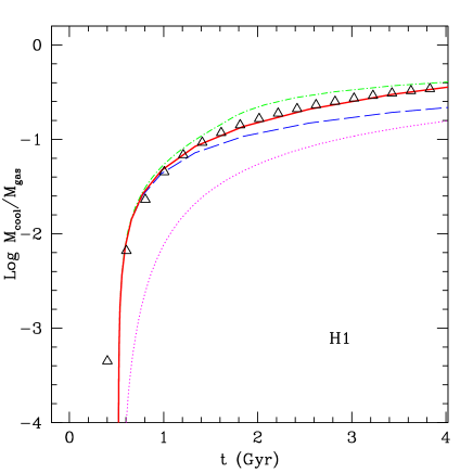
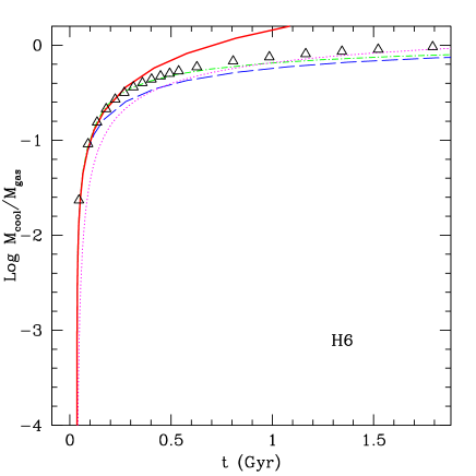
Figure 8: Simple approximation to the cooled mass fraction obtained by integrating in time the constant cooling flow of equation 41, shown for the H1 and H6 simulations (the others show a similar degree of agreement). Dotted (magenta), dashed (blue) and dot-dashed (green) lines give the predictions of the classical, unclosed and closed morgana models. The thick continuous line gives the simple analytic fit. For sake of completeness, the models are obtained using $\gamma_{p}=1.20$ and thermal energy equal to 1.18 times the virial energy (H1), and $\gamma_{p}=1.21$ and energy equal to 1.15 the virial energy (H6). These values are at the centre of the intervals used for the models shown in figure 7.

The last paragraph of Appendix A shows that, as long as the cooling radius sweeps the region where the gas density profile is shallower than $r^{-3/2}$, the cooling flow is roughly constant. Indeed, we find that both simulations and the morgana results can be fit with a constant cooling flow. To find an analytic approximation for it, we start from computing the reference radius $r_{\rm ref}$ at which $d\ln\rho_{g}/d\ln r=-3/2$. The function $\ln\rho_{g}$ (equation 3) is Taylor-expanded around $r_{s}$:

$$\rho_{g}(r_{s}) = \rho_{g0}\left[1-a\left(1-\ln 2\right)\right]^{1/(\gamma_{p}-1)}$$ (31)

$$\frac{d\ln\rho_{g}}{d\ln r}(r_{s}) = \frac{a}{\gamma_{p}-1}\,\frac{1/2-\ln 2}{1-a(1-\ln 2)}$$ (32)

$$\frac{d^{2}\ln\rho_{g}}{d\ln r^{2}}(r_{s}) = \frac{a}{\gamma_{p}-1}\,\frac{\ln 2-3/4+a(2-3\ln 2)/4}{[1-a(1-\ln 2)]^{2}}\,.$$ (33)

$$\ln\rho_{g}(r)\simeq\ln\rho_{g}(r_{s})$$

$$+\ln\left(\frac{r}{r_{s}}\right)\frac{d\ln\rho_{g}}{d\ln r}(r_{s})+\frac{1}{2}\left[\ln\left(\frac{r}{r_{s}}\right)\right]^{2}\frac{d^{2}\ln\rho_{g}}{d\ln r^{2}}(r_{s})+\ldots$$

The reference radius is then:

$$r_{\rm ref}\simeq r_{s}\exp\left(\frac{-3/2-d\ln\rho_{g}/d\ln r(r_{s})}{d^{2}\ln\rho_{g}/d\ln r^{2}(r_{s})}\right)$$ (35)

A guess for the reference cooling flow can then be obtained as $\dot{M}\simeq 4\pi r_{\rm ref}^{3}\rho_{g}(r_{\rm ref})/t_{\rm cool}(r_{\rm ref})$. This guess has been compared to the value of the cooling flow in the morgana unclosed and closed models, averaged over the time interval from 1 to 3 central cooling times and over the two models. We find systematic differences that are removed by adopting a correction function $f(M_{H},c_{\rm nfw})$ of halo mass and concentration. Let’s call:

$$A = 1.95-\left(\frac{1.41\times 10^{10}}{M_{H}}\right)^{0.3}$$ (36)

$$B = \max\left\{0.09\left[1-\left(\frac{M_{H}}{1.26\times 10^{15}}\right)^{0.3}\right],0.06\right\}$$ (37)

$$C = -0.043\left(B-0.085\right)+0.0014$$ (38)

then the correction function $f$ is found to be:

$$f(M_{H},c_{\rm nfw})=A+(c_{\rm nfw}-10)B$$ (39)

if $c_{\rm nfw}<=10$, and

$$f(M_{H},c_{\rm nfw})=A+(c_{\rm nfw}-10)B+(c_{\rm nfw}-10)^{2}C$$ (40)

if $c_{\rm nfw}>10$. The approximated cooling flow is then:

$$\dot{M}_{\rm approx}\simeq f(M_{H},c_{\rm nfw})\times\frac{4\pi r_{\rm ref}^{3}\rho_{g}(r_{\rm ref})}{t_{\rm cool}(r_{\rm ref})}$$ (41)

The dependence on cosmology is hidden in the dependence on redshift and concentration of $r_{\rm ref}$ and the function $f(M_{H},c_{\rm nfw})$.

This simple analytical model gives a very good fit to all the simulations shown in this paper, at least at early times. For sake of brevity, we show here (figure 8) only the reference H1 case and the worst-case H6 simulation. In the latter case the fraction of cooled mass approaches unity, and the approximation of a constant cooling flow breaks after $\sim 10$ central cooling times. It is very simple to truncate the constant cooling flow by imposing that the cooled mass does not overshoot the gas mass. However, a precise modeling of these late phases is immaterial, as feedback from star formation and AGNs would clearly regulate the dynamics of cooling, so any reasonable truncation would work equally well.

References

- Baugh (2006) Baugh C. M., 2006, Reports of Progress in Physics, 69, 3101
- Benson et al. (2001) Benson A. J., Pearce F. R., Frenk C. S., Baugh C. M., Jenkins A., 2001, MNRAS, 320, 261
- Bertschinger (1989) Bertschinger E., 1989, ApJ, 340, 666
- Cattaneo et al. (2007) Cattaneo A., Blaizot J., Weinberg D. H., Kereš D., Colombi S., Davé R., Devriendt J., Guiderdoni B., Katz N., 2007, MNRAS, 377, 63
- Cole et al. (2000) Cole S., Lacey C. G., Baugh C. M., Frenk C. S., 2000, MNRAS, 319, 168
- Fontanot et al. (2007) Fontanot F., Monaco P., Silva L., Grazian A., 2007, MNRAS, accepted, 0, 0
- Gnedin et al. (2004) Gnedin O. Y., Kravtsov A. V., Klypin A. A., Nagai D., 2004, ApJ, 616, 16
- Helly et al. (2003) Helly J. C., Cole S., Frenk C. S., Baugh C. M., Benson A., Lacey C., Pearce F. R., 2003, MNRAS, 338, 913
- Hernquist (1993) Hernquist L., 1993, ApJS, 86, 389
- Kauffmann et al. (1993) Kauffmann G., White S. D. M., Guiderdoni B., 1993, MNRAS, 264, 201
- Komatsu & Seljak (2001) Komatsu E., Seljak U., 2001, MNRAS, 327, 1353
- Menci et al. (2005) Menci N., Fontana A., Giallongo E., Salimbeni S., 2005, ApJ, 632, 49
- Monaco et al. (2007) Monaco P., Fontanot F., Taffoni G., 2007, MNRAS, 375, 1189
- Nagai & Kravtsov (2005) Nagai D., Kravtsov A. V., 2005, ApJ, 618, 557
- Nagamine et al. (2004) Nagamine K., Cen R., Hernquist L., Ostriker J. P., Springel V., 2004, ApJ, 610, 45
- Navarro et al. (1997) Navarro J. F., Frenk C. S., White S. D. M., 1997, ApJ, 490, 493
- Power et al. (2003) Power C., Navarro J. F., Jenkins A., Frenk C. S., White S. D. M., Springel V., Stadel J., Quinn T., 2003, MNRAS, 338, 14
- Romeo et al. (2005) Romeo A. D., Portinari L., Sommer-Larsen J., 2005, MNRAS, 361, 983
- Salpeter (1955) Salpeter E. E., 1955, ApJ, 121, 161
- Saro et al. (2006) Saro A., Borgani S., Tornatore L., Dolag K., Murante G., Biviano A., Calura F., Charlot S., 2006, MNRAS, 373, 397
- Somerville & Primack (1999) Somerville R. S., Primack J. R., 1999, MNRAS, 310, 1087
- Springel (2005) Springel V., 2005, MNRAS, 364, 1105
- Springel et al. (2006) Springel V., Frenk C. S., White S. D. M., 2006, Nature, 440, 1137
- Springel & Hernquist (2002) Springel V., Hernquist L., 2002, MNRAS, 333, 649
- Sutherland & Dopita (1993) Sutherland R. S., Dopita M. A., 1993, ApJS, 88, 253
- Suto et al. (1998) Suto Y., Sasaki S., Makino N., 1998, ApJ, 509, 544
- Tornatore et al. (2003) Tornatore L., Borgani S., Springel V., Matteucci F., Menci N., Murante G., 2003, MNRAS, 342, 1025
- White & Frenk (1991) White S. D. M., Frenk C. S., 1991, ApJ, 379, 52
- Yoshida et al. (2002) Yoshida N., Stoehr F., Springel V., White S. D. M., 2002, MNRAS, 335, 762