Optical afterglows of gamma–ray bursts: a bimodal distribution?

Abstract

The luminosities of the optical afterglows of Gamma Ray Bursts, 12 hours (rest frame time) after the trigger, show a surprising clustering, with a minority of events being at a significant smaller luminosity. If real, this dichotomy would be a crucial clue to understand the nature of optically dark afterglows, i.e. bursts that are detected in the X–ray band, but not in the optical. We investigate this issue by studying bursts of the pre–Swift era, both detected and undetected in the optical. The limiting magnitudes of the undetected ones are used to construct the probability that a generic bursts is observed down to a given magnitude limit. Then, by simulating a large number of bursts with pre–assigned characteristics, we can compare the properties of the observed optical luminosity distribution with the simulated one. Our results suggest that the hints of bimodality present in the observed distribution reflects a real bimodality: either the optical luminosity distributions of bursts is intrinsically bimodal, or there exists a population of bursts with a quite significant grey absorption, i.e. wavelength independent extinction. This population of intrinsically weak or grey–absorbed events can be associated to dark bursts.

1 Introduction

Since the detection of the first long Gamma Ray Burst (GRB) optical afterglow (Van Paradijs et al. 1997), the non–detection of any optical source in the direction of the gamma–ray trigger of some events stimulated the interest about the possible differences between the nature of the afterglow emission of the optically bright and faint GRBs. During the last 9 years the increasing number of optical detections and spectroscopic redshift determinations allowed us to study the intrinsic features of the optical afterglow emission of long GRBs. Despite the improved (i.e. made more promptly) observations of optical afterglows, in almost half of the observed long GRBs no optical counterpart is still found. These events have been called in the literature as Dark Burst, or Failed Optical Afterglows GRBs (Lazzati et al. 2002).

In Nardini et al. (2006a) we showed the optical $R$ band luminosity light curves of a sample of 24 pre–Swift GRBs with known spectroscopic redshift and published estimate of host galaxy dust absorption. We found a strong clustering of that luminosities for the GRBs in our sample. Most (i.e. 21/24) of the $R$ band luminosities at 12 hours in the source frame are clustered within a log–normal distribution centred around a mean value $\log L_{\nu_{R}}=30.65$ [erg s^-1 Hz^-1] with a dispersion $\sigma=0.28$. We also found 3 GRBs showing dimmer luminosities, a factor 15 (from 3.6 to 4.6 $\sigma$) smaller than the mean of the higher luminosity distribution. No GRB was found in the luminosity range between these two “families”. In Fig 1 we show the histogram of the $R$ band luminosities of our sample of GRBs.

In a recent update (Nardini et al. 2006b) we added 8 new GRBs detected by the Swift satellite (Gehrels et al. 2004) for whose an estimate of the host galaxy dust extinction has been published. This small sample of Swift GRBs confirms both the clustering and the bimodality of the optical luminosities found by us with pre–Swift bursts. We also evaluated the optical luminosities for 17 other Swift GRBs without any published $A_{V}^{host}$ estimate, and found that they are consistent with our previous findings.

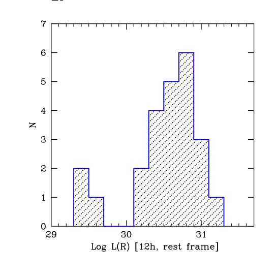
Figure 1: Histogram of the monochromatic optical luminosities 12 hours (rest frame) after the trigger for the 24 GRBs analysed in Nardini et al. (2006a). Data have been de-reddened both for Galactic and host extinction.

The discovery of a family of optically dim GRBs is an important clue for the understanding of the nature of dark bursts. The few underluminous observed events could be the tip of the iceberg of a population of GRBs which are intrinsically less luminous. Therefore, a fraction of dark GRBs could belong to this family whose distance, optical absorption, or observing conditions do not allow any optical detection. Because of its potential importance for the understanding of dark bursts, we investigate, in this paper, if the observed bimodal luminosity distribution of optically–bright bursts is due to any selection effect (related to the search/detection of GRB optical counterparts) or if it reflects the existence of two GRB populations.

To this aim we simulate through a Montecarlo method a sample of GRBs with a redshift distribution traced by the cosmic star formation rate (Porciani & Madau 2001), assuming different shapes of their intrinsic optical luminosity function. We also simulate different values of dust absorption within the host galaxy to all the simulated events. This value is calculated assuming the standard extinction curves (Pei 1992).

We infer a limiting magnitude distribution obtained by the analysis of the deepest $R$ band upper limits of all the pre–Swift GRBs with no detection of their optical afterglow. This is the key point of our study: the use of the upper limits on the optical flux to construct the probability that a simulated bursts would be detected or not. It is this probability distribution that allows us to perform, meaningfully, our simulations. We then compare the resulting luminosity distribution of the detectable simulated events with the one obtained in Nardini et al. (2006a) and shown in Fig 1.

The scope of our simulation is to check if for any conceivable combination of the input assumptions (i.e. luminosity function, extinction and redshift distribution) we can reproduce a simulated sample whose $R$–band luminosity distribution (12h rest frame) is consistent with that observed with the sample of 24 pre–Swift GRBs.

For our analysis we use only the pre–Swift GRBs because they represent an homogeneous sample: their optical light curves were sampled from hours to days after the trigger and the estimates of the host galaxy extinction have been published. The same study can be repeated using the more recent Swift GRBs once we will have a sufficient number of events with published estimates of the host galaxy extinction (now this number is too small, see Nardini et al. 2006b).

2 Optical upper limits of dark bursts

During over 7 years from the detection of the first long GRB optical afterglow in 1997 (Van Paradijs et al. 1997) to the launch of the Swift satellite on November 20th 2004 (Gherels et al. 2004), 238 long GRBs have been localised, within a few hours to days, with an accuracy of 1 degree or better. For only 64 of them an associated optical afterglow was found. For a large fraction of them the lack of optical data is due to the absence of any optical telescope pointing the source location error. We found 111 bursts with at least one optical–NIR failed (i.e. giving only a flux upper limit) observation and among them we focused our attention on the 94 GRBs with at least one $R$ band limiting magnitude.

In order to avoid including in our sample events with a large gamma–ray error box uncovered by the optical observation, we discarded the events with an error box wider than 11’ of radius if the $R$ band observation set does not cover at least the 80% of the error box area. We found 2 events which do not satisfy this criterion. For the others:

• 58 events have an error box narrower than 10’ of radius

• 27 events with the entire error box covered by the observations

• 4 events with more than 90% of the error box covered

• 3 events with more than 80% of the error box covered

We performed our analysis with these 92 dark GRBs.

We often found a large number of $R$ band upper limits for a single burst obtained at different epochs after the trigger. In these cases we evaluated the deepest limiting $R$ band magnitude for each GRB assuming a temporal behaviour $F(\nu,t)\propto t^{-\alpha}$ with $\alpha=1$, the average slope of the detected optical afterglows. For instance suppose that, for a given burst, there are two upper limits of $R>18$ and $R>20$ at, say, 1 and 24 hours since trigger, respectively. We select $R>18$ at 1 hour as the most stringent, since it corresponds [assuming $F(t)\propto t^{-1}$] to $R>21.45$ at 24 hours.

We corrected the resulting upper limits for the Galactic dust extinction along the line of sight using the absorption maps found by Schlegel et al. 1998. For most of the events the amount of Galactic dust absorption is negligible but there are some GRBs absorbed by several magnitudes in the $R$ band . For example, along the line of sight of GRB 030501 and GRB 030320, the Galactic dust absorption value $A_{R}$ (in the $R$ band) is 39 and 20.5 magnitudes, respectively. Such an extinction makes impossible any GRB optical afterglow detection.

In Fig. 2 we show the deepest $R$ band upper limits for all the 92 GRBs of the sample, de-reddened for the Milky Way dust absorption.

Figure 2: Deepest $R$ band upper limits for all the pre–Swift dark bursts. All the data are corrected for the Galactic extinction given in Schlegel et al. (1998). Each upper limit corresponds to a single GRB. For GRBs with several upper limits available in the literature, we report, conservatively, the deepest upper limit evaluated by assuming a standard flux decay light curve (see text).

2.1 Telescope Selection Function

For the majority of the dark GRBs in our sample, the deepest upper limit is quite constraining. Lazzati et al. (2002), albeit with a smaller sample of bright and dark GRBs, demonstrated that the non detection of an optical afterglow for most of the optically dark GRBs was not due to adverse observing conditions or delay in performing the observations. They also showed that these events do not have particularly large Galactic absorbing columns. The upper limits we added in our sample are generally deeper than the previous ones, thus confirming their results. Therefore, we can reasonably exclude that any instrumental bias is responsible for the failure of the detection of the optical afterglow in dark GRBs.

In order to obtain an homogeneous distribution of upper limits we extrapolated the deepest limiting $R$ band magnitude for each burst at the common time of 12 hours after the burst trigger (observer frame). We again assumed a temporal behaviour of the form $F\propto t^{-\alpha}$ with an index $\alpha=1$.

In Fig. 3 we show the $R$ band deepest limiting magnitudes for all the dark GRBs in our sample. The obtained values represent the distribution of the optical observation depth for a large number of events. Thanks to the consistency of the upper limits and the afterglow detections (see Lazzati et al. 2002), we can use this distribution to describe the probability for a burst to be observed in the optical with a certain depth. We can call this distribution Telescope Selection Function (TSF).

We can see in Fig. 3 that most of the dark bursts have been observed at 12 hours at least down to R$\approx$20. Sometimes the limiting magnitudes are greater than 24. Only for a small fraction of GRBs the limiting magnitude is smaller than 15, possibly due to bad observational conditions and/or high Galactic absorption.

Note that all the limiting magnitudes and the detected afterglow data considered in our sample concerns bursts observed before the launch of the Swift satellite. During the last two years, indeed, the prompt (within few minutes since trigger) location of the GRB allowed the early pointing of the optical telescopes. As a consequence, dark bursts observed in the Swift–era have systematically earlier upper limits than pre–Swift bursts. Besides, the early optical (and at a larger extent the early X–ray) light curves of several Swift bursts have shown unexpected features (different slopes, re-brightening and flares) whose nature is still debated. Moreover, the increased number of GRBs with accurate and promptly distributed positions makes it difficult to systematically extend the optical follow–up campaign up to few days after the trigger for all bursts. Therefore, on average, the available optical observations of Swift bursts are covering the very early optical afterglow emission, from few minutes to several hours since the burst onset. For these differences we prefer to keep separate the pre–Swift and the Swift bursts although the study that we propose in this paper, based on the sample of pre–Swift GRBs, can be performed with a sizable sample of Swift bursts with host extinction and late optical observations.

Figure 3: Histogram of the deepest $R$ band upper limits (corrected for Galactic extinction) extrapolated at a common time (12h after the trigger), obtained assuming a temporal behaviour $F(t)\propto t^{-1}$ of the optical afterglow flux. This distribution corresponds to the Telescope Selection Function (see text).

3 Simulated sample

The basic idea of our simulation is to produce, under some assumptions, a population of GRBs which is “subject” to the same TSF that we constructed from the upper limits of dark bursts. The result is a population of observed optical afterglows which can be compared with the real one. This is a test on the assumptions, of the simulated sample, i.e. (1) its redshift distribution, (2) the intrinsic luminosity function and (3) the host galaxy extinction.

3.1 Redshift distribution

The lack of optical information about the dark GRBs does not allow a direct spectroscopic redshift determination for all but two of them (GRB 000210, Piro et al 2002; GRB 000214, Antonelli et al. 2000). Assuming that the dark GRBs are related to the same progenitors of the optically detected bursts we can use the cosmic star formation (CSFR) history to represent the redshift distribution of all the GRBs we analyse. Among the three recipes of Porciani & Madau (2001), which differ at $z\geq$2, we considered the CSFR#2 (Eq.5 in that paper). The K–correction has been calculated assuming that the optical–UV afterglow spectrum is a single power law: $F(\nu)\propto\nu^{-\beta}$. The observed spectral index $\beta$ is usually in the range $0.5<\beta<1$. We used a typical value $\beta=1$ in our simulation but our results are unchanged if adopting different values in the range $0.5<\beta<1$ and choosing a different shape for the CSFR (e.g. Eq. 4 or 6 in Porciani & Madau (2001)).

3.2 Luminosity function

We assumed 3 different types of intrinsic monochromatic luminosity distributions at the common time 12 hours in the source frame: a log–normal, a powerlaw and a top–hat. For each luminosity function we considered several combination of their free parameters. Note that we cannot be guided, in the choice of the optical luminosity function, from what we already know of the luminosity function of the prompt emission of GRBs (see e.g. Firmani et al. 2004), since there is no correlation between the optical luminosity at 12 hours and the luminosity (or total energy) of the burst (see Nardini et al. 2006).

3.3 Host galaxy dust absorption

The association of long GRBs with massive progenitors could imply the presence of a large amount of absorbing dust in the source neighbourhood. On the other hand, the analysis of optical–near infrared afterglow spectral energy distributions showed a relatively small amount of reddening due to dust in the host galaxy. The value of $A_{V}^{host}$ in the source frame is usually of the order of a fraction of a magnitude (Kann et al. 2006; see Fig. 3 in Nardini et al. 2006a), despite the evidence of high $N_{\rm H}$ column densities found in the X–ray afterglow analysis (Vreeswijk et al. 2004; Jakobsson et al. 2006; Stratta et al. 2004).

We take into account the host galaxy dust absorption effects on the observable optical luminosities in our simulation. We test different shapes of the intrinsic $A_{V}^{host}$ distributions. The corresponding $A_{R}^{host}$ (in the rest frame) has been evaluated using the analytical extinction curves by Pei (1992). Most of the estimated dust absorption in optical GRB afterglows are well described by extinction curves without an evident 2175 Å feature, so we used a Small Magellanic Cloud like extinction curve. In any case, our results are not largely affected by this choice.

This sample of generated events is then assumed to be observed using optical telescopes with a limiting magnitudes distribution traced by the TSF at the common ($z=0$) time $t_{obs}=12h$. (Note that the effect of Galactic dust absorption is considered within the TSF definition). All events whose redshift makes the Ly–$\alpha$ break to obscure the observed $R$ band radiation have been considered as dark. In summary:

• we assume a redshift distribution function, a luminosity distribution and a host galaxy absorption function;

• we pick up at random a redshift $z$ a luminosity $L(R)$ and a host extinction $A_{V}$. With these parameters we compute the $R(12h)$ magnitude of the event at 12h in the observer frame;

• we pick up at random a limiting magnitude $R_{lim}(12h)$ for the telescope that will observe this event within the TSF.

• We compare $R(12h)$ with $R_{lim}(12h)$ to decide if this event can be observed or not. All events with redshift greater than 5 are considered undetectable.

In order to make a statistically meaningful simulation we repeat the above procedure 1000 times and build up the luminosity distribution of the “observable” events. This distribution can be finally compared with the observed one (Fig. 1). Through the comparison between the simulated “detectable” sample and the really observed one we can assign a probability to our set of assumptions. We can then repeat this procedure by changing the starting assumptions (e.g. the luminosity and/or absorption distribution).

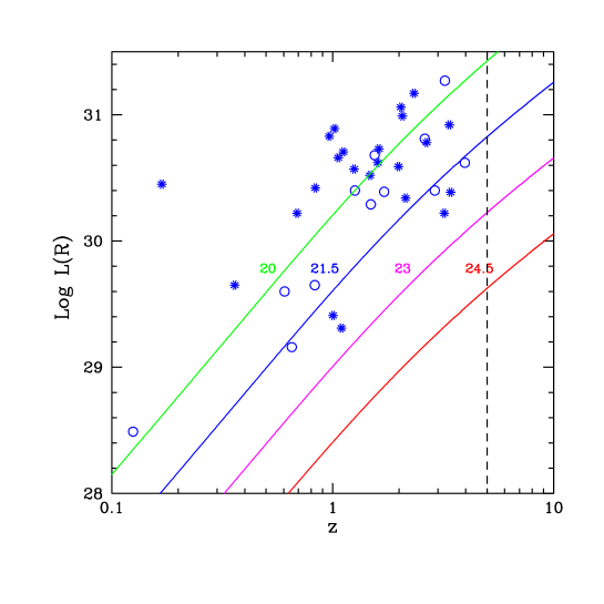
Figure 4: Limiting observable intrinsic $R$ band luminosity as a function of redshift, for different limiting magnitudes. Starred dots represent the luminosities of the GRBs in the sample and circles represent the Swift burst luminosities (Here we added 4 new Swift GRBs with a published estimate of $A_{V}^{host}$). The dashed vertical line at $z=5$ corresponds the Lyman–$\alpha$ break for the $R$ band.

4 Comparison with the observed distribution

The luminosity distribution of the simulated GRBs, that are observable using the considered TSF, has to be compared with the distribution of the observed GRB afterglows. Some features of the tested intrinsic luminosity functions have been chosen in order to better reproduce the distribution represented in Fig. 1. For example it is necessary to impose an high luminosity cut off to the luminosity function at about $\log[L(\nu_{R})^{12h}]\approx 31.2$ [erg s^-1Hz^-1]. A GRB with a greater luminosity would be easily detectable also with a low limiting magnitude for almost all the redshifts smaller than 5 (see Fig. 4). The absence of any observed GRB with such a luminosity therefore sets a constraint to the luminosity function.
The method most commonly adopted for comparing two distinct distributions is the two-sample Kolmogorov Smirnov (K-S) test. Unfortunately, given the specific luminosity distribution we are considering (Fig 1), this method has some critical limitations. Indeed (e.g. Press et al. 1992, Numerical Recipes in C, Second Edition; Ashman et al. 1994), the K-S test is ideal for comparing the median of two distributions but it is not sensitive to the tails of the distributions being compared and it also fails in comparing bimodal with unimodal distributions. In particular in our case we want to statistically verify a bimodality represented by an excess of events (i.e. the low luminosity events) which are located on the tail of the more numerous population of high luminosity bursts but at more than 3.6 $\sigma$ away from its central value. By applying the K-S test in order to compare an unimodal luminosity function with such an observed distribution we expect to strongly overestimate the null hypothesis probability. This is the reason why we have searched for a statistical method that fully exploited the observational constrain of having “a lack” of events with optical luminosities in between those of the two population of Fig.1.
We adopted the Likelihood Ratio Test (LRT) described by Cash 1979.
The simulation generates a sample of 30000 GRBs, each with an associated intrinsic luminosity $L(\nu_{R})$, redshift, host galaxy dust absorption $A_{V}^{host}$ and telescope limiting magnitude. The simulation returns the luminosities of the events that have an observer frame flux large enough to be detected by the associated telescope. Through this luminosities distribution we can predict the number of bursts expected in each bin using the same binning adopted in the histogram plotted in Fig. 1. We can then compare these predictions with the observed data by evaluating the factor C (eq.3 of Cash 1979) of the LRT. A large Cash statistic C implies the rejection of the model. As a reference value we adopted C=9.2 which corresponds to a probability of rejection of the model hypothesis of $P_{rej}=90$%. A simulated distribution can be considered consistent with the observed data with $P_{rej}<90$% if the obtained C is smaller than 9.2.

Table 1: Simulation results without considering host galaxy absorption

a	b	$C^{c}$	$CP^{d}$	$P_{KS}^{e}$
G	30.65, 0.25	35.5	$<10^{-5}$	0.38
G	30.20, 0.70	14.8	$6.1\cdot 10^{-4}$	0.31
G	30.50, 0.50	15.4	$4.5\cdot 10^{-4}$	0.69
TH	29.3, 31.2	12.0	$2.5\cdot 10^{-3}$	0.33
PL	29.3, 31.2, $-$1	11.7	$2.9\cdot 10^{-3}$	0.24
PL	29.3, 31.2, $-$1.5	11.7	$2.9\cdot 10^{-3}$	0.24
PL	29.3, 31.2, $-$2	11.6	$3.0\cdot 10^{-3}$	0.22

a) Assumed luminosity distribution: G=Gaussian, TH=top hat, PL=power–law.
b) Parameters G: $\mu$, $\sigma$; TH: minimum luminosity, maximum luminosity; PL: minimum luminosity, maximum luminosity, index $\alpha$ assuming $N\propto L(\nu_{R})^{\alpha}.$
c) Value of the C factor obtained with the Cash statistics.
d) Cash Probability from eq. 3 (Cash 1979).
e) Probability obtained with the K-S test.

5 Results

5.1 Simulation without considering host galaxy dust absorption

We considered different combinations of the parameters characterising the assumed luminosity distribution (i.e. mean value $\mu$ and $\sigma$ for the log–normal, luminosity range and slope $\alpha$ for the power–law and the luminosity range for the top hat). The results of the simulations are listed in Tab. LABEL:noabs We found that in none of these cases the observed luminosity distribution of the simulated samples agrees with the observed one. The factor C is always larger than 11.6. In the log–normal cases, a narrow luminosity function that well matches the observed high luminosity peak returns a large C value because it cannot reproduce the low luminosity excess. A too wide distribution has, instead, an excess of events with $\log{L(\nu_{R})^{12h}}>31.2$, in contrast with the observed maximum luminosity.

Both the power–law and the top hat distributions are affected by similar problems. The observed high luminosity cut off requires an upper bound to the simulated distributions. The low luminosity end instead does not affect our results. As it happens for the log–normal distribution, we are unable to reproduce an observable luminosity distribution, since we always violate some of the observed properties of the distribution shown in Fig 1.

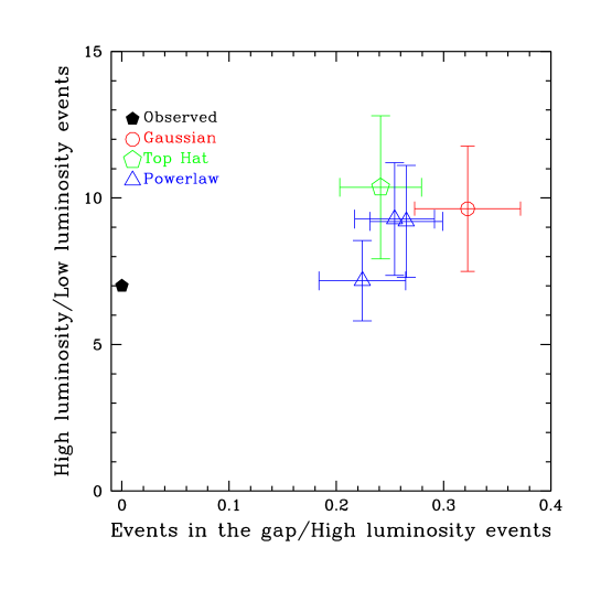
Figure 5: Unabsorbed case. Ratio between the number of observed events with $30.2<\log[L(\nu_{R})^{12h}]<31.2$ and $\log{L(\nu_{R})^{12h}}<29.7$ versus the observed events with $29.7<\log{L(\nu_{R})^{12h}}<30.2$ and $30.2<\log[L(\nu_{R})^{12h}]<31.2$ for the considered initial luminosity functions in case of host galaxy dust absorption absence. Error bars show 1 $\sigma$ uncertainties.

As an illustrative exercise we show in Fig. 5 the results obtained by repeating 1000 times the former simulation with 1000 events. We plot the ratio between the number of observed events in the high ($30.2<\log[L(\nu_{R})^{12h}]<31.2$ over the low ($29.7<\log{L(\nu_{R})^{12h}}<30.2$) luminosity bins versus the ratio of the number of observed events in the gap ($29.7<\log{L(\nu_{R})^{12h}}<30.2$) and those in the high luminosity range ($30.2<\log[L(\nu_{R})^{12h}]<31.2$). Note that the the ratios of the simulated samples stand at more than 3$\sigma$ from the observed one (filled pentagon).

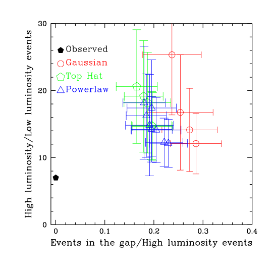
Figure 6: Host galaxy absorption case. Ratio between the number of observed events with $30.2<\log[L(\nu_{R})^{12h}]<31.2$ and $\log{L(\nu_{R})^{12h}}<29.7$ versus the observed events with $29.7<\log{L(\nu_{R})^{12h}}<30.2$ and $30.2<\log[L(\nu_{R})^{12h}]<31.2$ for the different initial luminosity functions considering the host galaxy dust absorption effects. Error bars show 1 $\sigma$ uncertainties.

5.2 Host galaxy absorption

In order to check if the addition of the host galaxy dust absorption allows us to produce a luminosity distribution compatible with the observed one, we tested some different kinds of absorption distributions and extinction curves. The distribution of $A_{V}^{host}$ estimated for the observed bursts is dominated by low values. A large number of events are consistent with zero absorption and the majority of them show $A_{V}^{host}$ smaller than 1 magnitude. This however could be due to selection effects, since it is more difficult to detect highly absorbed optical sources.

We first assumed a top hat $A_{V}^{host}$ distribution, with a minimum $A_{V}^{host}=0$, and assuming different maximum absorption values (i.e. $A_{V,Max}^{host}=2,3,5$ magnitudes). Then we simulated a power–law like $A_{V}^{host}$ distribution (with different slopes and $A_{V,Max}^{host}$), which better represents the observed distribution. We finally assumed a single value for the $V$ band extinction in the host galaxy for all bursts (note that this conditions in any case implies different values of $A_{\nu_{R}(1+z)}$). We also tried a Gaussian distribution, but the results are very similar to those found with the top hat distribution.

For all these attempts we have combined the $A_{V}^{host}$ distributions with the different luminosity distributions described in the previous section. The results are listed in Tab. LABEL:siabs. In no case we were able to reproduce the observed distribution. We conclude that a continuous absorption distribution, combined with a unimodal luminosity function, is unable to generate an observable GRBs luminosity distribution characterised by an empty gap between the two different luminosity groups.

Table 2: Simulation results considering different shapes of host galaxy dust absorption distributions.

Luminositya	Parametersa	Absorptionb	$C^{a}$	$CP^{a}$	$P_{KS}^{a}$
distribution		parameters
G	30.65, 0.25	TH, 2	32.3	$<10^{-5}$	0.16
G	30.20, 0.70	TH, 2	14.4	$7.5\cdot 10^{-4}$	0.20
G	30.50, 0.50	TH, 2	17.1	$1.9\cdot 10^{-4}$	0.23
G	30.65, 0.25	P, 2, $-$1	35.4	$<10^{-5}$	0.25
G	30.65, 0.25	P, 2, $-$2	63.8	$<10^{-5}$	0.28
G	30.20, 0.70	P, 2, $-$1	14.3	$7.8\cdot 10^{-4}$	0.49
G	30.20, 0.70	P, 2, $-$2	14.7	$6.4\cdot 10^{-4}$	0.35
G	30.50, 0.50	P, 2, $-$1	15.3	$4.8\cdot 10^{-4}$	0.50
G	30.50, 0.50	P, 2, $-$2	14.6	$6.8\cdot 10^{-4}$	0.61
G	30.65, 0.28	C, 0.5	34.2	$<10^{-5}$	0.16
G	30.20, 0.70	C, 0.5	13.9	$9.6\cdot 10^{-4}$	0.23
G	30.50, 0.50	C, 0.5	18.2	$1.1\cdot 10^{-4}$	0.24
G	30.65, 0.28	C, 0.7	33.3	$<10^{-5}$	0.14
G	30.20, 0.70	C, 0.7	14.2	$8.3\cdot 10^{-4}$	0.14
G	30.50, 0.50	C, 0.7	17.5	$1.6\cdot 10^{-4}$	0.17
TH	29.3, 31.2	TH, 2	11.6	$3.0\cdot 10^{-3}$	0.56
TH	29.3, 31.2	P,2, $-$1	12.1	$2.4\cdot 10^{-3}$	0.48
TH	29.3, 31.2	P,2, $-$2	12.3	$2.1\cdot 10^{-3}$	0.35
TH	29.3, 31.2	C, 0.5	11.8	$2.7\cdot 10^{-3}$	0.58
TH	29.3, 31.2	C, 0.7	12.6	$1.8\cdot 10^{-3}$	0.44
PL	29.3, 31.2, $-$1	TH, 2	11.0	$4.1\cdot 10^{-3}$	0.75
PL	29.3, 31.2, $-$1	P, 2, $-$1	11.5	$3.2\cdot 10^{-3}$	0.41
PL	29.3, 31.2, $-$1	C, 0.7	10.4	$4.5\cdot 10^{-3}$	0.64
PL	29.3, 31.2, $-$1	C, 0.5	11.3	$3.5\cdot 10^{-3}$	0.73
PL	29.3, 31.2, $-$2	TH, 2	10.6	$5.0\cdot 10^{-3}$	0.77
PL	29.3, 31.2, $-$2	P, 2, $-1$	11.2	$3.7\cdot 10^{-3}$	0.77
PL	29.3, 31.2, $-$2	C, 0.5	10.9	$4.3\cdot 10^{-3}$	0.78
PL	29.3, 31.2, $-$2	C, 0.7	10.7	$4.7\cdot 10^{-3}$	0.71

a) Same notes as in Tab. LABEL:noabs.
b) Absorption distributions parameters. TH: maximum absorption in the $V$ band magnitudes (the minimum is set to 0); P: maximum absorption in the $V$ band magnitudes and index $\alpha$; C: constant absorption $A_{V}^{host}$.

Table 3: Simulation results assuming an achromatic “grey dust” absorption

Luminositya	Parametersa	Absorptiona	Grey dustb	$A_{\lambda}$c	$C^{a}$	$CP^{a}$	$P_{KS}^{a}$
distribution		parameters	%
G	30.65, 0.25	0	60	1.6	6.0	$5.0\cdot 10^{-2}$	0.40
G	30.65, 0.25	0	70	1.6	4.4	0.11	0.69
TH	30.2, 31.2	0	60	1.5	5.6	$6.1\cdot 10^{-2}$	0.35
TH	30.2, 31.2	0	70	1.5	4.7	$9.5\cdot 10^{-2}$	0.21
PL	30.2, 31.2, $-$1	0	70	1.5	2.9	0.24	0.50
PL	30.2, 31.2, $-$2	0	70	1.5	2.6	0.27	0.51

a) Same notes as in Tab. LABEL:siabs.
b) Fraction of the simulated events with an associated achromatic rest frame absorption (in percentage).
c) Achromatic absorption amount (in magnitudes).

5.3 Achromatic extinction

The analysis of the optical to X–ray spectral energy distributions (SED) of some long GRBs suggests the presence of an achromatic optical absorption component (Stratta et al. 2005), perhaps due to the small size grain destruction in the neighbourhood of the GRB (Lazzati et al. 2001, Perna & Lazzati 2002). The amount of this absorption could be higher than what inferred assuming standard dust (even by several magnitudes). We then considered the possibility that a fraction of GRBs can be absorbed with an achromatic extinction curve. Starting with the same luminosity function tested in the previous cases, we associated a further achromatic absorption to a fraction of events. Such an absorption decreases the observable flux and the chance for those events to be detected. When observed, the analysis of the optical SED of these GRBs would not show any evidence of dust absorption. The inferred intrinsic luminosity could therefore be underestimated by a factor equal to the grey absorption amount. The optical luminosity distribution inferred by the observer could appear bimodal even if the real intrinsic luminosity function were unimodal.
This last absorption model, when applied in the simulation to a large fraction of events, returns often a luminosity distribution compatible with the observed one. For the cases tested in this paper the C factor is always smaller than 9.2. Indeed it is even smaller than 4.6 (P=90%) reaching in some cases very small values with P$<$24%. We conclude that unimodal luminosity functions can reproduce the observed bimodal luminosity distribution of fig. 1, if strong achromatic absorption is assumed.

Similarly to what we have done in Fig. 5 we plot in Fig. 7 the high to low luminosity number ratio vs the gap to high luminosity number ratio. For clarity, we inserted in this plot only the cases with grey absorption only, without the addition of a standard dust absorption effect. As can be seen, there are luminosity functions (powerlaw and top–hat) which agree with the observed luminosity distribution.

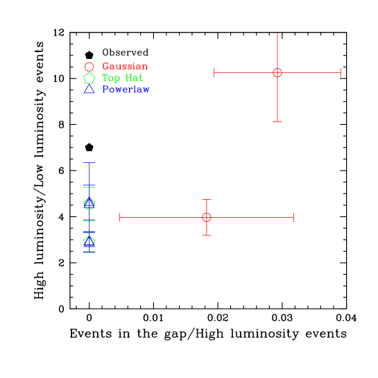
Figure 7: Achromatic absorption case. Ratio between the number of observed events with $30.2<\log[L(\nu_{R})^{12h}]<31.2$ and $\log{L(\nu_{R})^{12h}}<29.7$ versus the observed events with $29.7<\log{L(\nu_{R})^{12h}}<30.2$ and $30.2<\log[L(\nu_{R})^{12h}]<31.2$ for the different initial luminosity functions in the case of achromatic dust absorption. In all the plotted points we did not consider the contribution of the standard dust absorption. Error bars show 1 $\sigma$ uncertainties.

6 Discussion

Our findings suggests that the bimodality of the observed optical luminosity distribution, even if found with a relatively small number of events, is significant. It can be the result of either a bimodality in the optical luminosity function, or the result of a fraction of bursts being absorbed by a significant amount of grey dust.

In the first case we would expect that the bimodality in the optical afterglow luminosity is accompanied by some hints of bimodality in other properties, such as the energetics of the prompt emission or the luminosity distribution of the X–ray afterglow flux. However, as already discussed in Nardini et al. (2006a), there are no convincing evidences of such a behaviour. Indeed, it was just this lack of evidence that prompted us to consider the alternative hypothesis of grey absorption. In this case, however, we have to assume the presence of a relatively large amount of grey dust (producing an absorption of 1.5–2 magnitudes) only in a fraction of bursts. Our results are therefore difficult to understand, implying, in any case, the existence of two, relatively well separated, GRB optical afterglow families. Note that infrared observations, while surely important and crucial to confirm the existence of the clustering of the high luminosity burst class and the separation in two luminosity classes, would not discriminate between the two hypotheses mentioned above. In fact, since the grey dust is absorbing the observed infrared flux (which would be optical or UV in the rest frame) by the same amount of the observed optical one, we could not distinguish between an intrinsic bimodal luminosity distribution and the presence of grey dust. To this aim it will be useful in the future an extended broadband afterglow analysis of the optically subluminous events. On the other hand infrared observations and spectroscopy would not be limited to bursts having $z<5$, and could therefore give important information on the number of bursts above this redshift limit, where the different star formation rates greatly differ. It will then be possible to directly measure the number of bursts which are optically dark because they lie at large redshifts. In Fig. 8, we superposed the simulated events to the plot shown in Fig. 4. In this case we simulated two separate Gaussian luminosity functions characterised by the same width but with different mean values (i.e. 30.65 and 29). The starred dots represent the observed values updated with the Swift GRBs, the small triangles represent the non detectable simulated events and the empty pentagons represent the observable simulated ones. This figure shows how such a bimodal optical luminosity function well reproduces the distribution obtained with the real data.

Our results have important implications for the nature of dark GRBs. In the pre-Swift era it was possible to infer a redshift for at least 3 Dark GRBs (i.e. 970828, 000210 & 000214). In Nardini et al. (2006a) we showed that the X-Ray and Gamma-Ray energetics of GRB 000210 and GRB 000214 are comparable to the optically subluminous ones. The Galactic absorption corrected R band upper limits of GRB 000210 and of GRB 970828 are deep enough to infer upper limits for their intrinsic optical luminosities that are much smaller than the observed events ones (i.e. $\log{L(\nu_{R})}<28.7$ at 8.9h after trigger rest frame for GRB 000210 and $\log{L(\nu_{R})}<28.4$ at 3.2h after trigger rest frame). Lazzati et al. 2002 excluded that most of the long Dark GRBs have no optical detection because of “adverse” observing conditions, since their associated limiting optical magnitudes are not particularly small (i.e. the corresponding flux limits are severe). Therefore it is very likely that dark bursts belong to the observed optically underluminous family, whose “existence” has been statistically proved in this work. If it is intrinsically faint or affected by a large achromatic extinction is still to be found.

We did our study using a sample of bursts belonging to the pre–Swift era. As stated, we are forced to do that, because of the paucity of Swift events with measured (and published) values of the host galaxy extinction. Once we will have enough bursts, we can repeat our analysis with Swift bursts, which will shed light on the link between the optical afterglow properties at relatively late times (12 hours in the rest frame) and the early afterglow properties. For the moment, we can only stress that all Swift bursts for which the host galaxy extinction has been measured entirely confirm the observed bimodality in the optical luminosity distribution.

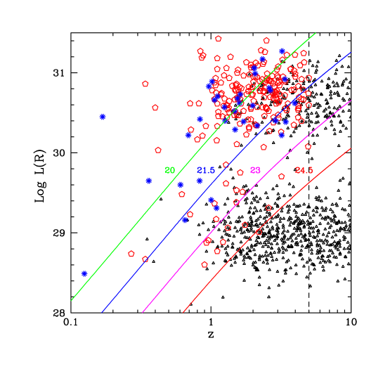
Figure 8: Logarithm of the optical luminosity $\log L(\nu_{R})^{12h}$ versus redshift $z$ for the observed GRBs updated with the ones detected by Swift (starred dots), for the undetectable simulated events (small triangles) and for the observable simulated events (empty pentagon).

7 Summary and conclusions

In this study we analysed the possible importance of observational selection effects on the clustering and the bimodality found in the long GRBs optical afterglow luminosity distribution.

• We studied the $R$ band upper limits of all the pre–Swift dark GRBs and we showed that they are consistent with the “typical” afterglow detections. The distribution of these upper limits extrapolated at 12 h after trigger enables the definition of a Telescope Selection Function, which can define the probability, for any burst, to be pointed with a telescope and exposure time corresponding to some limiting magnitude.

• Through Montecarlo simulations, we have studied which combinations of optical luminosity functions and absorption in the host galaxy can be consistent with the observations. In doing so, we have found that the gap between the two observed luminosity distribution is real and it is not the result of a small number statistics.

• If the absorption is chromatic (i.e. a “standard” one) no unimodal intrinsic luminosity distribution agrees with the observed one. If a good fraction of events (but not all) is absorbed by “grey” (i.e. achromatic) dust, then a unimodal luminosity distribution is possible. An achromatic absorption would not be recognised through the standard $A_{V}^{host}$ estimate methods. This can lead to underestimate the intrinsic luminosity for a fraction of bursts that could thus appear as members of an underluminous family.

• Dark bursts could then be associated either to an intrinsically optically underluminous family, or to those bursts being characterised by a relatively large achromatic absorption. In the first case one should explain why, optically, the luminosity distribution is bimodal, while other properties are not (e.g. the distribution of the energetics of the prompt emission), while in the second case one should explain why a fraction of bursts live in a different environment, characterised by grey dust.

8 Appendix 1
Reference for the upper limits of the dark burst

GRB970111: Castro-Tirado et al. (1997); GRB970228: Odewahn et al. (1997); GRB981220: Pedersen et al. (1999); GRB990217: Palazzi et al. (1999); GRB990506: Vrba et al.(1999); GRB990527: Pedersen et al. (1999b); GRB990627: Rol et al. (1999); GRB990704: Rol et al. (1999b); GRB990806: Greiner et al. (1999); GRB990907: Palazzi et al. (1999b); GRB991014: Uglesich et al. (1999); GRB991105: Palazzi et al. (1999c); GRB991106: Jensen et al. (1999); GRB000115: Gorosabel et al. (2000); GRB000126: Kjernsmo et al. (2000); GRB000210: Gorosabel et al. (2000b); GRB000307: Kemp et al. (2000); GRB000323: Henden et al. (2000); GRB000326: Pedersen et al. (2000); GRB000408: Henden et al. (2000b); GRB000416: Price et al. (2000); GRB000424: Uglesich et al. (2000); GRB000508B: Jensen et al. (2000); GRB000519: Jensen et al. (2000b); GRB000528: Palazzi et al. (2000); GRB000529: Palazzi et al. (2000b); GRB000607: Masetti et al. (2000); GRB000615: Stanek et al. (2000); GRB000616: Bartolini et al. (2000); GRB000620: Gorosabel et al. (2000c); GRB000623: Gorosabel et al. (2000d); GRB000801: Palazzi et al. (2000c); GRB000812: Masetti et al. (2000b); GRB000830: Jensen et al. (2000c); GRB001018: Bloom et al. (2000); GRB001019: Henden et al. (2000c); GRB001025: Fynbo et al. (2000); GRB001105: Castro Ceron et al. (2000); GRB001109: Greiner et al. (2000); GRB001120: Price et al. (2000b); GRB001204: Price et al. (2000c); GRB001212: Zhu (2000); GRB010103: Dillon et al. (2001); GRB010119: Price et al. (2001); GRB010126: Masetti et al (2001); GRB010213: Zhu (2001); GRB010220: Berger et al. (2001); GRB010324: Oksanen et al (2001); GRB010326A: Price et al. (2001b); GRB010326B: Pandey et al. (2001); GRB010412: Price et al. (2001c); GRB010629: Halpern et al. (2001); GRB011019: Komiyama et al. (2001); GRB011030: Rhoads et al. (2001); GRB011212: Saracco et al. (2001); GRB020127: Castro Cerón et al. (2002); GRB020409: Price et al. (2002); GRB020418: Gorosabel et al. (2002); GRB020531: Dullighan et al., (2002); GRB020603: Castro Cerón et al. (2002b); GRB020604: Gorosabel et al. (2002b); GRB020625: Price et al. (2002b); GRB020812: Ohashi et al. (2002); GRB020819: Levan et al. (2002); GRB021008: Castro-Tirado et al. (2002); GRB021016: Durig et al. (2002); GRB021112: Schaefer et al. (2002); GRB021113: Kawabata et al. (2002); GRB021201: Garnavich et al. (2002); GRB021204: Ishiguro et al. (2002); GRB021206: Pedersen et al. (2003); GRB021219: Castro-Tirado et al. (2002b); GRB030204: Nysewander et al. (2003); GRB030320: Gal-Yam et al. (2003); GRB030413: Schaefer et al. (2003); GRB030414: Lipunov et al. (2003); GRB030416: Henden et al. (2003); GRB030501: Klotz et al. (2003); GRB030823: Fox et al. (2003); GRB030824: Fox et al. (2003b); GRB030913: Henden et al (2003); GRB031026: Chen et al. (2003); GRB031111: Silvey et a. (2003); GRB040223: Gomboc et al. (2004); GRB040228: Sarugaku et al. (2004); GRB040403: de Ugarte et al. (2004); GRB040624: Fugazza et al., (2004); GRB040701: de Ugarte et al. (2004b); GRB040810: Price et al. (2004); GRB040812: Cobb et al. (2004); GRB040825A: Jensen et al. (2004); GRB040825B: Gorosabel et al. (2004); GRB041015: Isogai et al. (2004); GRB041016: Kuroda et al. (2004); GRB041211: Monfardini et al. (2004);

References

- [] Antonelli, L.A., Piro, L., Vietri, M., et al., 2000, ApJ, 535, 39
- [] Ashman, K.M., Bird, C.M. & Zepf, S.E., 1994, A.J., 108,2348
- [] Bartolini, C., Gualandi, R., Guarnieri, A., Piccioni, A., Palazzi, N., Pian, E. & Masetti, N., 2000, GCN, 714
- [] Berger, E., Frail, D.A., Price, P.A., Bloom, J.S., Galama, T.J., Kudritzki, R. & Bresolin, F., 2001, GCN, 958
- [] Bloom, J.S., Diercks, A., Kulkarni, S.R., Harrison, F.A., Behr, B.B. & Clemens, J.C., 2000, GCN, 915
- [] Cash, W., 1979, ApJ, 228, 939
- [] Castro Ceron, J.M., Castro-Tirado, A.J., A. Henden, A., et al., 2000, GCN, 894
- [] Castro Ceron, J.M., Gorosabel, J., Amado, P. & Castro Cerón, J.M., 2002, GCN, 1775
- [] Castro Ceron, J.M., Gorosabel, J., Greiner, J., Klose, S., Snigula, J. & Castro-Tirado, A.J., 2002, GCN, 1234
- [] Castro Ceron, J.M., Pedani, M., Gorosabel, J. & Castro-Tirado, A.J., 2002b, GCN, 1413
- [] Castro-Tirado, A.J. & Gorosabel, J., 1997, IAUC, 6598
- [] Castro-Tirado, A.J., Klose, S., Wisotzki, L., Greiner, L., Castro Ceron, J.M. & Gorosabel, J., 2002, GCN, 1642
- [] Chen, A.C., Ting,H.C., Lin, H.C., Huang, K.Y., Kinoshita, D., Ip, W.H., Urata, Y. & Tamagawa, T., 2003, GCN, 2436
- [] Cobb, B.E. & Bailyn, C.D., 2004, GCN, 2642
- [] de Ugarte Postigo, A., Sota, A., Gorosabel, J. & Castro-Tirado, A.J., 2004, GCN, 2571
- [] de Ugarte Postigo, A., Tristram, P., Sasaki, Gorosabel, J., Yock, P. & Castro-Tirado, A.J., 2004, GCN, 2621
- [] Dillon, B. & Dellinger, J., 2001, GCN, 911
- [] Dullighan, A., Monnelly, G., Butler, N., Vanderspek, R., Ford, P. & Ricker, G., 2002, GCN, 1411
- [] Durig, D.T., Shroyer, E.W., Shukla, P.P. & West, D., 2002, GCN, 1644
- [] Firmani, C., Avila-Reese, V., Ghisellini, G. & Tutukov, A., 2004, ApJ, 611, 1033
- [] Fox, D.B., & Hunt, M.P., 2003, GCN, 2365
- [] Fox, D.B., & Hunt, M.P., 2003b, GCN, 2369
- [] Fugazza, D., D’Avanzo, P., Tagliaferri, G., et al., 2004, GCN, 2617
- [] Fynbo, J.P.U., Moller, P., Milvang-Jensen, B., et al., 2000, GCN, 867
- [] Gal-Yam, A. & Ofek, E.O., 2003, GCN, 1946
- [] Garnavich, P. & Quinn, J., 2002, GCN 1746
- [] Gehrels, N., Chincarini, G., Giommi, P., et al., 2004, ApJ, 601, 1005
- [] Gomboc, A., Marchant, J.M., Smith, R.J., Mottram, C.J. & Fraser, S.N., 2004, GCN, 2534
- [] Gorosabel, J., de Ugarte Postigo, A., Miranda, L.F., Jelinek, M., Pereira, C.B., Castro Cerón, J.M. & Aceituno, J., 2004, GCN, 2675
- [] Gorosabel, J., Henden, A., Castro-Tirado, A.J., et al., 2000c, GCN, 734
- [] Gorosabel, J., Hjorth, J., Jakobsson, P., et al., 2002, GCN, 1419
- [] Gorosabel, J., Hjorth, J., Jensen, B.L., Pedersen, H., Jakobsson, P., Fynbo, J. & Andersen, M.I., 2002b, GCN, 1429
- [] Gorosabel, J., Jensen, B.L., Hjorth, J., Fogh Olsen, L., Christensen, L., Andersen, M.I. & Jaunsen, A.O., 2000b, GCN, 547
- [] Gorosabel, J., Pascual, S., Gallego, J., et al., 2000d, GCN, 735
- [] Gorosabel, J., Vrba, F., Henden, A., et al., 2000, GCN, 563
- [] Greiner, J., Pompei, J., Els, S., et al., 1999, GCN, 396
- [] Greiner, J., Stecklum, B., Klose, S., et al., 2000, GCN, 887
- [] Halpern, J.P. & Mirabal, N., 2001, GCN, 1079
- [] Henden, A., Castro-Tirado, A.J. & Castro Ceron, J.M., 2000, GCN, 621
- [] Henden, A., Kaiser, D., Hohman, D., Pason, R. & Aquino, B., 2000c, GCN, 858
- [] Henden, A., Luginbuhl, C., Canzian, B., 2000b, GCN, 633
- [] Henden, A. & Oksanen, A., 2003, GCN, 2392
- [] Henden, A., Silvay, J., Moran, J., Soule, R., Reichart, D., Schaefer, J., Canterna, R. & Scoggins, B., 2003, GCN, 2250
- [] Ishiguro, M., Sarugaku,Y., Nonaka, H., Kwon, S.M., Nishiura, S., Mito, H. & Urata, Y., 2002, GCN, 1747
- [] Ishiguro, M., Mizuno, T., Arai, Y., Sato, F., Urata, Y., Tamagawa, T. & Huang, K.Y., 2004, GCN, 2825
- [] Jakobsson, P., Fynbo, J.P.U., Ledoux, C., et al., 2006, astro-ph, 0609450
- [] Jensen, B.L., Cassan, A., Dominis, D., et al., 2004, GCN, 2686
- [] Jensen, B.L., Pedersen, H., Hjorth, J., et al., 2000, GCN, 670
- [] Jensen, B.L., Pedersen, H., Hjorth, J., Gorosabel, J., Dall, T.H. & O’Toole, S., 2000b, GCN, 679
- [] Jensen, B.L., Pedersen, H., Hjorth, J., Gorosabel, J., Fynbo, J.P.U. & Nowotny, W., 2000c, GCN, 788
- [] Jensen, B.L., Pedersen, H., Hjorth, J., Larsen, S. & Costa, E., 1999, GCN, 440
- [] Kawabata, T., Ayani, K., Yamaoka, H., Kawai, N. & Urata, Y., 2002, GCN, 1700
- [] Kann, D.A., Klose, S., Zeh, A., 2006, ApJ, 641, 993
- [] Kemp, J. & Halpern, J.P., 2000, GCN, 609
- [] Kjernsmo, K., Jaunsen, A., Saanum, OE, Jensen, B.L., Hjorth, J., Pedersen, H. & Gorosabel, J., 2000, GCN, 533
- [] Klotz,A. & Boër, M., 2003, GCN, 2224
- [] Komiyama, Y., Kosugi, G., Kobayashi, N., et al., 2001, GCN, 1128
- [] Kuroda, D., Yanagisawa, K & Kawai, N., 2004, GCN, 2818
- [] Lazzati, D., Covino, S. & Ghisellini, G., 2002, MNRAS, 330, 583
- [] Lazzati, D., Perna, R. & Ghisellini, G., 2001, MNRAS, 325, 19
- [] Levan, A., Burud, I., Fruchter, A., Rhoads, J., van den Berg, A., Homan, J., Rol, E. & Tanvir, N., 2002, GCN, 1517
- [] Liang, E. & Zhang, B., 2006, ApJ, 638, 67
- [] Lipunov, L., Krylov, A., Kornilov, V., et al., 2003, GCN, 2157
- [] Masetti, N., Palazzi, E., Pedani, M., Magazzu, A., Ghinassi, F. & Pian, E., 2001, GCN, 926
- [] Masetti, N., Palazzi, E., Pian, E., et al., 2000, GCN, 720
- [] Masetti, N., Palazzi, E., Pian, E., Cosentino, R., Ghinassi, F., Magazzú, A. & Benetti, S., 2000b, GCN, 774
- [] Monfardini, A., Guidorzi, C., Mottram, C.J. & Mundell, C., 2004, GCN, 2852
- [] Nardini, M., Ghisellini, G., Ghirlanda, G., Tavecchio, F., Firmani, C. & Lazzati, D., 2006a, A&A, 451, 821
- [] Nardini, M., Ghisellini, G., Ghirlanda, G., Tavecchio, F., Firmani, C. & Lazzati, D., 2006b, submitted to Il Nuovo Cimento
- [] Nysewander, M., Henden, A., Lopez-Morales, M., Reichart, D. & Schwartz, M., 2003, GCN, 1861
- [] Odewahn, S.C., Djorgovski, S.G., Kulkarni, S. R. & Frail, D.A., 1997, IAUC, 6730
- [] Ohashi, H., Kato, T., Senda, T., Mii, H., Mizuno, K., Yasaka, Y. & Yamaoka, H., 2002, GCN, 1515
- [] Oksanen, A., Hyvonen, H., Price, A., et al., 2001, GCN, 1019
- [] Palazzi, E., Masetti, N., Pian, E., et al., 1999, GCN, 262
- [] Palazzi, E., Masetti, N., Pian, E., et al., 2000, GCN, 691
- [] Palazzi, E., Masetti, N., Pian, E., et al., 2000b, GCN, 699
- [] Palazzi, E., Masetti, N., Pian, E., et al., 2000c, GCN, 767
- [] Palazzi, N., Pian, E., Masetti, N., et al., 1999b, GCN, 413
- [] Palazzi, N., Pian, E., Masetti, N., et al., 1999c, GCN, 449
- [] Pandey, S.B., Stalin, C.S. & Mohan, V., 2001, GCN, 1040
- [] Pedersen, Jensen, B.L., Hjorth, J. & Gorosabel, J., 2000, GCN, 625
- [] Pedersen, Jensen, B.L., Järvinen, A. & Andersen, M.I., 2003, GCN, 2350
- [] Pedersen, H., Lindgren, B., Hjorth, J., Andersen, M.I., Jaunsen, A.O., Sollerman, J., Smoker, J. & Mooney, C., 1999, GCN, 192
- [] Pedersen, H., Hjorth, J., Jensen, B. L., Rasmussen, M. B., Jaunsen, A. O. & Hurley, K., 1999b, GCN, 139
- [] Pei, Y.C., 1992, ApJ, 395, 130
- [] Perna, R. & Lazzati, D., 2002, ApJ, 580, 261
- [] Piro, L., Frail, D.A., Gorosabel, J., et al., 2000, ApJ, 571, 680
- [] Porciani, C. & Madau, P., 2001, ApJ, 548, 522
- [] Press, W.H., Teukolosky, S.A., Vetterling, W.T. & Flannery, B.P., 1992,Numerical Recipes in C, Second Edition, Cambridge University Press, Page 626.
- [] Price, P., Axelrod, T. & Schmidt, B., 2000, GCN, 640
- [] Price, P., Axelrod, T. & Schmidt, B., 2000c, GCN, 898
- [] Price, P., Axelrod, T. & Schmidt, B., 2001c, GCN, 1038
- [] Price, P., Axelrod, T., Schmidt, B. & Reichart, D.E., 2001b, GCN, 1022
- [] Price, P., Hauser, M., Pühlhofer, G. & Wagner, S.J., 2004, GCN, 2639
- [] Price, P., Hunt, M.P. & Fox, D.W., 2002, GCN, 1368
- [] Price, P., Meltzer, J., Stalder, B., Djorgovski, S.G. & Galama, T.J., 2000b, GCN, 892
- [] Price, P., Morrison, G. & Bloom, J.S., 2001, GCN, 919
- [] Price, P., Schmidt, B., Axelrod, T. & Bloom, J.S., 2002b, GCN, 1441
- [] Rhoads, J.E., Burud, I., Fruchter, A., Kouveliotou, C. & Wood-Vasey, M., 2001, GCN, 1140
- [] Rol, E., Palazzi, E., Masetti, N., et al., 1999, GCN, 358
- [] Rol, E., Vreeswijk, P., Galama, T., et al., 1999b, GCN, 374
- [] Saracco, P., Covino, S., Ghisellini, S., 2001, GCN, 1205
- [] Sarugaku, Y., Aoki, T., Urata, Y., Huang, K.Y. & Tamagawa, T., 2004, GCN, 2537
- [] Schaefer, J., Gibbs, D., Nysewander, M., Canterna, R. & Reichart, D., 2003, GCN, 2137
- [] Schaefer, J., Savage, S., Canterna, R., Nysewander, M., Reichart, D., Henden, A. & Lamb,D., 2002, GCN, 1776
- [] Schlegel, D.J., Finkbeiner, D.P. & Davis, M., 1998, ApJ, 500, 525
- [] Silvey, J., Allen,D., Canterna, R. & Price, P.A., 2003, GCN, 2447
- [] Stanek, K.Z., Garnavich, P.M. & Berlind, P., 2000, GCN, 706
- [] Stratta, G., Fiore, F., Antonelli, L.A., Piro, L. & De Pasquale, M., 2004, ApJ, 608, 846
- [] Stratta, G., Perna, R., Lazzati, D., Fiore, F., Antonelli, L.A., Conciatore, M.L., 2005, A&A, 441, 83
- [] Uglesich, R., Halpern, J. & Thorstensen, J., 1999, GCN, 428
- [] Uglesich, R., Mirabal, N., Halpern, J.P., Vanlandingham, K., Noel-Storr, J., Wagner, R.M. & Eskridge, P., 2000, GCN, 663
- [] Van Paradijs, J., Groot, P.J., Galama, T., et al., 1997, Nature, 386, 682
- [] Vrba, F.J., Henden, A.A., Canzian, B., et al., 1999, GCN, 305
- [] Vreeswijk, P.M., Ellison, S.L., Ledoux, C., et al., 2004, A&A, 419, 927
- [] Zhu, J., 2000, GCN, 904
- [] Zhu, J., 2001, GCN, 946