Astrophysical Condition on the attolensing as a possible probe for
a modified gravity theory

Abstract

We investigate the wave effect in the gravitational lensing by a black hole with very tiny mass less than $10^{-19}M_{\rm sun}$ (solar mass), which is called attolensing, motivated by a recent report that the lensing signature might be a possible probe of a modified gravity theory in the braneworld scenario. We focus on the finite source size effect and the effect of the relative motion of the source to the lens, which are influential to the wave effect in the attolensing. Astrophysical condition that the lensed interference signature can be a probe of the modified gravity theory is demonstrated. The interference signature in the microlensing system is also discussed.

I Introduction

Many physicists have drawn attention to extra dimensional physics for several years due to recent development in testing Randall-Sundrum type II (RS-II) scenario RSII . In this scenario they considered a four dimensional positive-tension brane embedded in five dimensional AdS bulk which allows us to reconsider our understanding about the history of our universe in the early stages. Some investigations have been carried out to modify the existence of primordial black holes (PBH)s in this RS-II scenario that the life time of five dimensional PBHs against the Hawking radiation becomes longer compared with the standard PBH in four dimensions GCL . This is because the five dimensional feature becomes significant in the black hole with very tiny mass. The ratio of the life time against the Hawking radiation of such five dimensional PBH to that of the four dimensional PBH may be estimated, $lM_{4}/l_{4}M$, where $l$ is the AdS radius of the braneworld model, $l_{4}$ and $M_{4}$ are the four dimensional Planck length and mass, respectively, and $M$ is the black hole mass GCL .

Since the braneworld PBHs can live longer, then it is possible that such black holes still exist and spread out in our universe. Therefore, it is natural to consider the possibility of the gravitational lensing phenomenon by such the black hole. More recently, the authors KPIII investigated the wave effect in gravitational lensing by the black hole with the very tiny mass smaller than $10^{-19}M_{\rm sun}$, where $M_{\rm sun}$ is the solar mass, which is called attolensing. They showed that the interference signature in the energy spectrum in gamma ray burst due to the attolensing might be a possible probe of the modified gravity theory. In the standard general relativity, PBH with the mass smaller $10^{-18}M_{\rm sun}$ will be evaporated through the Hawking radiation within the cosmic age. Then, the detection of such the interference signature would be a probe of extra dimension of our universe.

In the present paper, we consider the two effects in the lensing phenomenon that are influential for measurement of the interference signature in the energy spectrum in the attolensing: One is the finite source size effect. The other is the effect of the relative motion of the black hole (lens object) to the source. We demonstrate the condition that these effects become influential. This is one of the astrophysical conditions that the attolensing can be a probe of the modified gravity theory. Throughout this paper, $H_{0}=72$ km s^-1 Mpc^-1 is the Hubble parameter, and we use the unit in which the light velocity equals 1.

II Review of Basic Equations

The wave effect in the gravitational lensing has been investigated (e.g., SEF ; Nakamura ; path ). We start with a brief review of the black hole solution in the type II Randall-Sundrum braneworld gravity model. We write the line element as KPIII ; GT

$$ds2=-(1+2\Psi)dt^{2}+(1+2\Phi)d{\bf x}^{2},$$ (1)

where

$$\Psi=-{GM\over r}-{2\over 3}{GMl^{2}\over r^{3}},$$ (2)

$$\Phi=+{GM\over r}+{1\over 3}{GMl^{2}\over r^{3}},$$ (3)

where $M$ is the black hole mass, $G$ is the gravitational constant, and $l$ is the AdS radius of the braneworld model. The propagation of the electromagnetic wave can be approximated by the massless scalar wave equation, which yields

$$\left(\triangle+\omega^{2}\right)\phi=(\Psi-\Phi)\phi,$$ (4)

where we assumed the amplitude of the field is in proportion to $e^{-i\omega t}\phi({\bf x})$, and $\omega$ is the angular frequency of the wave. With defined

$$\tilde{\psi}=\int dr\left(\Psi-\Phi\right)=4GM\ln\rho-2{GMl^{2}\over\rho^{2}}+{\rm constant},$$ (5)

the amplification factor is (e.g.,SEF ; Nakamura ; path )

$$F = {\omega\over 2\pi i}{D_{L}D_{S}\over D_{LS}}\int d^{2}\vec{\theta}\exp\left[i\omega\left({D_{L}D_{S}\over D_{LS}}\biggl{|}\vec{\theta}-\vec{\theta}_{0}\biggr{|}^{2}-\tilde{\psi}\right)\right],$$ (6)

where, $\vec{\theta}_{0}$ denotes the position of the source, $D_{S}$ is the (angular diameter) distance between the observer and the source, $D_{L}$ is the distance between the observer and the lens, and $D_{LS}$ is the distance between the lens and the source. Introducing the Einstein angle,

$$\theta_{E}=\sqrt{4GMD_{LS}\over D_{S}D_{L}},~{}~{}$$ (7)

and the dimensionless variables

$${\bf x}={\vec{\theta}\over\theta_{E}},~{}~{}{\bf y}={\vec{\theta}_{0}\over\theta_{E}},~{}~{}$$ (8)

and

$$w=4GM\omega,~{}~{}\varepsilon_{l}={l\over\theta_{E}D_{L}},$$ (9)

we have

$$F={w\over 2\pi i}\int d^{2}{\bf x}\exp\left[iw\left({1\over 2}|{\bf x}-{\bf y}|^{2}-\ln|x|+{\varepsilon_{l}^{2}\over 2|x|^{2}}\right)\right].$$ (10)

In the limit of the geometric optics, the light path is determined by the lens equation,

$$x-y-{1\over x}-{\varepsilon_{l}^{2}\over x^{3}}=0.$$ (11)

From KPIII , the solution is approximately obtained as

$$x={1\over 2}\left(\sqrt{4+y^{2}}\pm|y|\right)+{1\over 2}\left({2+y^{2}\over\sqrt{4+y^{2}}}\mp|y|\right)\varepsilon_{l}^{2}.$$ (12)

Then, the magnification is

$$|\mu^{\pm}|={1\over 2}\left({2+y^{2}\over|y|\sqrt{4+y^{2}}}\pm 1\right)-{2\over|y|\sqrt{4+y^{2}}^{3}}\varepsilon_{l}^{2},$$ (13)

and the time delay is

$${\Delta\tau}={1\over 2}|y|\sqrt{4+y^{2}}+\ln\left({\sqrt{4+y^{2}}+|y|\over\sqrt{4+y^{2}}-|y|}\right)+{\varepsilon_{l}^{2}\over 2}|y|\sqrt{4+y^{2}}.$$ (14)

In the semiclassical limit, the magnification is given by

$${\cal M}(w,y)=|F|^{2}\simeq{2+y^{2}\over|y|\sqrt{4+y^{2}}}+{2\over|y|\sqrt{4+y^{2}}}\sin(\omega\Delta\tau)-{4+2(2+y^{2})\sin(w\Delta\tau)\over|y|\sqrt{4+y^{2}}^{3}}{\varepsilon_{l}^{2}}.$$ (15)

The first term of the right hand side of Eq. (15) corresponds to the formula within the geometric optics, and the second term does to the semiclassical correction of the wave optics, and the third term does to the correction due to the modification of the gravity.

As discussed in the literature KPIII , one can write

$$\varepsilon_{l}^{2}\sim 10^{-18}\biggl{(}{l\over 0.2{\rm mm}}\biggr{)}^{2}\biggl{(}{M\over 10^{15}{\rm g}}\biggr{)}^{-1}\biggl{(}{H_{0}^{-1}\over D_{LS}D_{L}/D_{S}}\biggr{)}.$$ (16)

Thus the correction is small for the primordial braneworld black hole. Then, in the following, we neglect the correction of order $\varepsilon^{2}_{l}$.

III Finite source size effect

In this section, we consider the finite source size effect, which can be influential to the interference signature MY ; SPG . The magnification of a source with a finite size can be expressed by averaging the point source magnification over the source-position,

$$\bar{{\cal M}}(w)={\displaystyle{\int d^{2}{\bf y}W({\bf y}){\cal M}(w,y)}\over\displaystyle{\int d^{2}{\bf y}W({\bf y})}},$$ (17)

where $W({\bf y})$ denotes the distribution of the source intensity. In this paper, we assume the uniform intensity of a circular region, for simplicity,

$$W({\bf y})=\left\{\begin{array}[]{ll}1{}{}{}&{\rm for}~{}~{}~{}~{}|{\bf y}-{\bf y}_{0}|\leq R,\\ 0{}{}{}&{\rm for}~{}~{}~{}~{}|{\bf y}-{\bf y}_{0}|>R,\end{array}\right.$$ (20)

where ${\bf y}_{0}$ is the position of the center of the source and $R$ is the radius of the source.

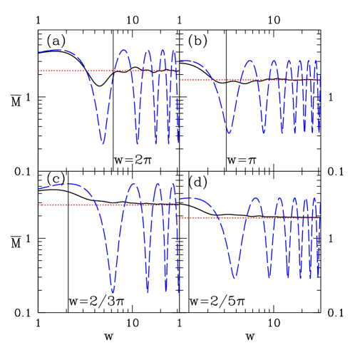
Figure 1: $\bar{\cal M}(w)$ (solid curve) as function of $w$ with $W({\bf y})$ shown in each panel in Figure 2, correspondingly. The dashed curve is ${\cal M}(w,y_{0})$, and the doted line is $\bar{\cal M}_{\rm geo}$.

We demonstrate the behavior of ${\bar{\cal M}}(w)$ as function of $w$ in several cases of $W({\bf y})$. The panels of Figure 1 show $\bar{\cal M}(w)$ for the source distribution function $W({\bf y})$, as shown in the panels of Figure 2, correspondingly. The radius, $R$ and the center-position of extended source $(|{\bf y}_{0}|)$ are $(R,|{\bf y}_{0}|)=(0.25,0.5)$ for the panel (a), $(0.5,0.75)$ for the panel (b), $(0.75,0.25)$ for the panel (c), $(1.25,0.25)$ for the panel (d), respectively. The dashed circle in the panel of Figure 2 is the Einstein radius.

In each panel of Figure 1, the solid curve is $\bar{\cal M}(w)$ defined by Eq. (17), but the dotted straight line is the result of the geometric optics,

$$\bar{{\cal M}}_{\rm geo}={\displaystyle{\int d^{2}{\bf y}W({\bf y})\Bigl{(}{|\mu^{+}(y)|+|\mu^{-}(y)|}}\Bigr{)}\over\displaystyle{\int d^{2}{\bf y}W({\bf y})}}.$$ (21)

The dashed curve in each panel of Figure 1 shows the magnification ${\cal M}(w,y_{p})$ of the point source located at the position $y_{p}$, where $y_{p}$ is determined by solving

$$\bar{\cal M}_{\rm geo}=|\mu^{+}(|y_{p}|)|+|\mu^{-}(|y_{p}|)|={2+|y_{p}|^{2}\over|y_{p}|\sqrt{4+y_{p}^{2}}},$$ (22)

which yields

$$y_{p}^{2}=-2+\frac{2{\bar{\cal M}}_{\rm geo}}{\sqrt{{{\bar{\cal M}}_{\rm geo}}^{2}-1}}.$$ (23)

Note that the behavior of $\bar{{\cal M}}(w)$ is similar to ${\cal M}(w,y_{p})$ for $w\sim 1$, while $\bar{{\cal M}}(w)$ approaches to $\bar{{\cal M}}_{\rm geo}$ as $w$ becomes larger, $w\gg 1$.

IV Relative motion of lens

In this section we consider the point source, but taking the relative motion of the source to the lens into account. Because black holes have naturally the velocity dispersion in the universe, then the position of the source relative to the lens moves within a finite observation time. Assuming that the time resolution to obtain the energy spectrum is not very fine and that the energy spectrum is obtained by the formula (17), but with

$$W({\bf y})=\left\{\begin{array}[]{ll}\displaystyle{\int dt\delta^{(2)}({\bf y}-{\bf y}(t)){}{}{}}&{\rm for}~{}~{}~{}~{}t_{ini}\leq t\leq t_{fin},\\ 0{}{}{}&{\rm for}~{}~{}~{}~{}t<t_{ini},~{}t>t_{fin},\end{array}\right.$$ (26)

where ${\bf y}={\bf y}(t)$ defines the track of the source. Substituting (26) into (17), we have

$$\bar{\cal M}(w)={\displaystyle{\int_{t_{ini}}^{t_{fin}}dt{\cal M}(w,y(t))}\over\displaystyle{\int_{t_{ini}}^{t_{fin}}dt}}.$$ (27)

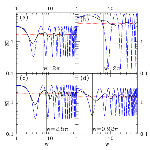
Figure 3: $\bar{\cal M}(w)$ (solid curve) as function of $w$ with $W({\bf y})$ shown in each panel in Figure 4, correspondingly. The dashed curve is ${\cal M}(w,y_{0})$, and the doted line is $\bar{\cal M}_{\rm geo}$.

The panels of Figure 4 show the typical tracks of the source $W({\bf y})$ considered here. Figure 3 shows the magnification corresponding to the tracks. The track is defined by the straight line connecting two points between $(0.5,0)$ and $(1,0)$ for the panel (a), $(0.1,0)$ and $(0.6,0)$ for the panel (b) $(0.5,0)$ and $(0.5,0.75)$ for the panel (c) $(0.5,0)$ and $(0.5,1.5)$ for the panel (d), respectively. The meaning of the solid, dotted, and dashed curve is same as those of Figure 1.

Similar to the case of the extended source, $\bar{{\cal M}}(w)$ takes similar value of ${\cal M}(w,y_{p})$, for $w\sim 1$. While $\bar{{\cal M}}(w)$ approaches to $\bar{{\cal M}}_{\rm geo}$ as $w$ becomes large, $w\gg 1$. However, note that the convergence of $\bar{{\cal M}}(w)$ to $\bar{{\cal M}}_{\rm geo}$ in the region $w\gg 1$ is slow in comparison with the case of the extended source in the previous section.

V Condition of phase cancellation

From the formulas (15) and (17), we expect that the interference signature disappears under the condition,

$$w|\Delta\tau(y_{\rm min})-\Delta\tau(y_{\rm max})|\lower 2.15277pt\hbox{$\;\buildrel>\over{\sim}\;$}2\pi,$$ (28)

where $y_{\rm min}$($y_{\rm max}$) is the minimum (maximum) value of $y$ in the (typical) region of the source defined by $W(\bf y)$. This condition means that the phase difference between the waves from $y_{\rm min}$ and $y_{\rm max}$ in the source plane is larger than $2\pi$. Namely, Eq. (28) is the condition of the phase cancellation.

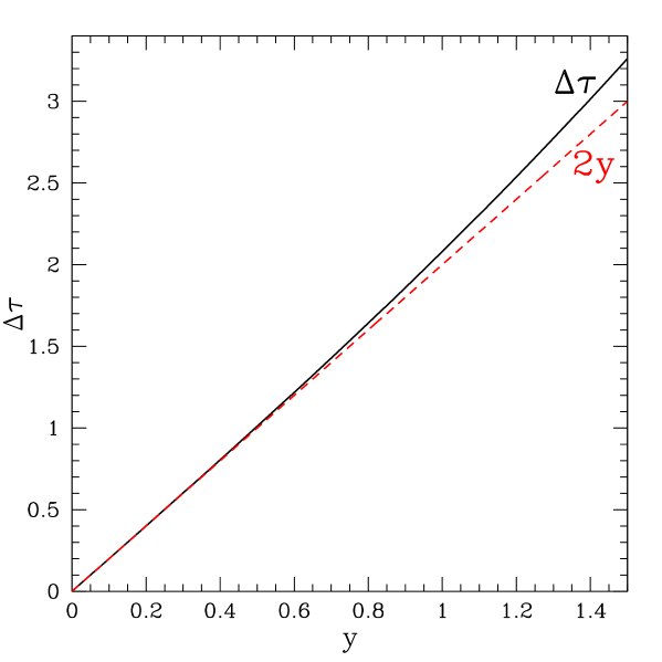
Figure 7: $\tau$ (solid curve) as a function $y$. The dashed line is $2y$.

In the case of the point-mass lens, formula (28) can be approximated in a simpler formula, as follows. Figure 7 shows $\Delta\tau(y)$ as a function of $y$. This suggests that $\Delta\tau=2y$ is a quite good approximation as long as $y\lower 2.15277pt\hbox{$\;\buildrel<\over{\sim}\;$}1$, inside the Einstein radius. This is understood by the Taylor expansion of $\tau(y)$,

$$\tau(y)=2\left[y+{1\over 24}y^{3}-{1\over 640}y^{5}+{\cal O}(y^{7})\right],$$ (29)

which suggests that the correction to the relation $\tau(y)=2y$ from the higher order terms is small as long as $y\lower 2.15277pt\hbox{$\;\buildrel<\over{\sim}\;$}1$. Then, (28) is written as

$$w|y_{\rm min}-y_{\rm max}|\lower 2.15277pt\hbox{$\;\buildrel>\over{\sim}\;$}\pi.$$ (30)

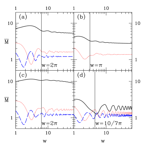
Figure 5: $\bar{\cal M}(w)$ as function of $w$ with $W({\bf y})$ shown in each panel in Figure 6, correspondingly.

The panels of Figure 5 show the magnification assuming $W({\bf y})$ shown in each panel of Figure 6, correspondingly. In each panel of Figure 6, we consider a few case of $W({\bf y})$ with the same $|y_{\rm max}-y_{\rm min}|$ but with different position of the center. In the panel (a), $W({\bf y})$ assumes the circles with $R=0.25$ and $|{\bf y}_{0}|=0.25~{}{\rm(solid~{}curve)},~{}0.75{\rm~{}(dotted~{}curve)},~{}1.25{\rm~{}(dashed~{}curve)}$, respectively. These sources have the same value $|y_{\rm max}-y_{\rm min}|=0.5$. In this case, from Eq. (30), the condition that the interference signature disappears is $w\gtrsim 2\pi$. One can confirm that the interference signature disappears at $w\gtrsim 2\pi$ from the panel (a) of Figure 5. Similarly, the panel (b) assumes the circles with the radius $R=0.5{\rm~{}(solid~{}curve)},1.0{\rm~{}(dotted~{}curve)}$, where Eq. (30) gives $w\gtrsim\pi$. Thus, Eq. (30) is regarded as the condition that the interference signature disappears due to the phase cancellation.

On the other hand, the panel (c) assumes the tracks of a point source which connect the two points between $(0.01,0)~{}{\rm and}~{}(0.51,0)$ (solid curve), $(1.0,0)~{}{\rm and}~{}(1.5,0)$ (dotted  curve), and $(0.5,0)~{}{\rm and}~{}(1,0)$ (dashed curve). All these cases have $|y_{\rm max}-y_{\rm min}|=0.5$, and Eq. (30) yields $w\gtrsim 2\pi$. Similarly, the panel (d) assumes the tracks of a point source which connect the two points, $(0.4,0)~{}{\rm and}~{}(0.4,\sqrt{1.1^{2}-0.4^{2}})$ (solid curve), $(0.8,0)~{}{\rm and}~{}(0.8,\sqrt{1.5^{2}-0.8^{2}})$ (dotted curve), and $(1.2,0)~{}{\rm and}~{}(1.2,\sqrt{1.9^{2}-1.2^{2}})$ (dashed curve). All these cases have $|y_{\rm max}-y_{\rm min}|=0.7$, and Eq. (30) yields $w\gtrsim 10\pi/7$. In these cases, the interference signature slightly remains even for $w|y_{\rm max}-y_{\rm min}|\gtrsim\pi$, but becomes very weak there.

In the reference MY , it is discussed that the finite source size effect becomes substantial and the interference signature is affected under the condition $wR\gg 1$. Eq. (30) is essentially same as the condition discussed in the previous paper.

VI Discussion

Here let us discuss the astrophysical condition that the finite source size effect becomes important in the attolensing. From the condition (30), we have

$$\hat{R}(1+z_{L})\omega\sqrt{4GMD_{L}\over D_{LS}D_{S}}\lower 2.15277pt\hbox{$\;\buildrel>\over{\sim}\;$}\pi,$$ (31)

where we introduced $\hat{R}(=|y_{\rm min}-y_{\rm max}|\theta_{E}D_{S})$, which is the physical size of the source, and the redshift of the lens is taken into account. Here we imagine the black holes spread throughout the Universe, and consider the attolensing at the cosmological distance. In this case Eq. (31) is rephrased as

$$1.1\times(1+z_{L})\biggl{(}{\hbar\omega\over{\rm 100MeV}}\biggr{)}\biggl{(}{M\over 10^{-19}{M_{\rm sun}}}\biggr{)}^{1/2}\biggl{(}{\hat{R}\over 10^{3}{\rm km}}\biggr{)}\biggl{(}{H_{0}^{-1}\over D_{LS}D_{S}/D_{L}}\biggr{)}^{1/2}\lower 2.15277pt\hbox{$\;\buildrel>\over{\sim}\;$}\pi.$$ (32)

Note that $10^{-19}M_{\rm sun}=0.2\times 10^{15}{\rm g}$. Thus the finite source size effect will be influential to the attolensing by the black hole at the cosmological distances, for example, $\hat{R}$ must be less than $10^{3}$ km. However, for the attolensing by the black hole at the galactic scale $D_{L}\sim 10{\rm~{}kpc}$ and $D_{LS}\sim D_{S}\sim H_{0}^{-1}$, the condition is relaxed by the factor $\sqrt{D_{S}/D_{L}}\sim 10^{3}$.

When the source has the relative velocity to the lens, $v_{\scriptscriptstyle\bot}$, perpendicular to the line of sight direction, we may write

$$|y_{\rm min}-y_{\rm max}|\simeq{v_{\scriptscriptstyle\bot}\Delta t\over D_{S}\theta_{E}},$$ (33)

where $\Delta t$ is the duration time of the source emission. From the condition (30),

$$(1+z_{L})\omega\sqrt{4GMD_{L}\over D_{DS}D_{S}}v_{\scriptscriptstyle\bot}\Delta t\gtrsim\pi.$$ (34)

Then, the condition (30) is written as

$$0.3\times(1+z_{L})\biggl{(}{\hbar\omega\over 100{\rm MeV}}\biggr{)}\biggl{(}{M\over 10^{-19}{M_{\rm sun}}}\biggr{)}^{1/2}\biggl{(}{\Delta t\over 1{\rm s}}\biggr{)}\biggl{(}{v_{\scriptscriptstyle\bot}\over 3\times 10^{2}{\rm km}}\biggr{)}\biggl{(}{{H_{0}^{-1}}\over D_{S}D_{LS}/D_{L}}\biggr{)}^{1/2}\lower 2.15277pt\hbox{$\;\buildrel>\over{\sim}\;$}\pi.$$ (35)

Thus, the relative motion of the source will be also influential to the attolensing by the black hole at the cosmological distance as well as at the galactic distance.

VII Summary and Conclusions

We investigated the condition that the finite source size effect and the relative motion of the source becomes substantial in the wave effect of the gravitational lensing. The condition is expressed by the formula (30), whose physical meaning is that the difference of the phase between the two light paths from $y_{\rm max}$ and $y_{\rm min}$ is larger than $2\pi$. We have shown that the finite source size effect is important in the attolensing by the black hole at the cosmological distance. Also the relative motion of the source to the lens can be influential. For the attolensing by the black hole at the galactic distance, the constraint is relaxed by the factor $\sqrt{D_{S}/D_{L}}\sim 10^{3}$. However, we should also note that the detection of the attolensing is limited in practice KPIII , even when the finite source size is not taken into account.

In general, the signature of the interference becomes remarkable when $w\sim 1$, i.e.,

$$w\sim 0.3\times(1+z_{L})\left({h\nu\over 100{\rm MeV}}\right)\left({M\over 10^{-19}M_{\rm sun}}\right)\sim 1.$$ (36)

In the case $w\lower 2.15277pt\hbox{$\;\buildrel<\over{\sim}\;$}1$, the amplification due to the lensing becomes negligible, because the wavelength of the light becomes larger than the size of deflector. Combining this and the condition (30), we may conclude that the condition for the possible observation of the interference signature in the gravitational lensing needs

$$1\lower 2.15277pt\hbox{$\;\buildrel<\over{\sim}\;$}w\lower 2.15277pt\hbox{$\;\buildrel<\over{\sim}\;$}{\pi\over|y_{\rm min}-y_{\rm max}|}.$$ (37)

Therefore, this means $|y_{\rm min}-y_{\rm max}|\lower 2.15277pt\hbox{$\;\buildrel<\over{\sim}\;$}\pi$, the angular size of the source must be less than the Einstein radius, is always necessary for a possible observation of the interference signature. It will be useful to demonstrate the region satisfying (37) clearly. In Figure 8, the dashed line is $w=1$, and the solid line is $w|y_{\rm min}-y_{\rm max}|=\pi$, where we fixed $\hat{R}=10^{3}$ km and $D_{LS}D_{S}/D_{L}=H_{0}^{-1}$. The shaded region satisfies the condition (37).

It might also be interesting to consider whether other physical system satisfy the condition (37) or not. Figure 9 shows a region satisfying the condition with the parameter associated with the microlensing. Similar to Figure 8, the shaded region satisfies the condition. Here the dashed line in Figure 9 is $w=1$, and the solid line is $w|y_{\rm min}-y_{\rm max}|=\pi$, where we fixed $\hat{R}=7\times 10^{5}$ km (solar radius) and $D_{LS}D_{S}/D_{L}=30$ kpc. The point of the intersection of these two lines is

$$\left({\nu\over{\rm GHz}}\right)=8.9\times 10^{2}\left({\hat{R}\over 7\times 10^{5}{\rm km}}\right)^{-2}\left({30{\rm kpc}\over D_{LS}D_{S}/D_{L}}\right)^{-1}$$ (38)

$$\left({M\over M_{\rm sun}}\right)=0.9\times 10^{-8}\left({\hat{R}\over 7\times 10^{5}{\rm km}}\right)^{2}\left({30{\rm kpc}\over D_{LS}D_{S}/D_{L}}\right).$$ (39)

Thus the microlensing can be a possible system that satisfies the condition (37). Especially, for the microlensing by an Earth like planet $M\sim 10^{-5}M_{\rm sun}$, the relevant range of the frequency is $1$ GHz $\sim 100$ GHz. Then, the measurement of the microlensing event through the frequency might be relevant to the interference signature. However, it will be very difficult to detect the signal because the stars at $1\sim 100$ GHz frequency band at the galactic distance is very dark in general.

Figure 2: The function $W({\bf y})$, where the region $W({\bf y})=1$ is shown by shaded region. The dashed circle is the Einstein radius.

Figure 4: The function $W({\bf y})$, where the region $W({\bf y})\neq 1$ is shown by straight line. The dashed circle is the Einstein radius.

Figure 6: The each panel shows $W({\bf y})$. The dashed circle is the Einstein radius.

Figure 8: The dashed line is $w=1$, and the solid line is $w|y_{\rm min}-y_{\rm max}|=\pi$, where we fixed $\hat{R}=10^{3}$ km and $D_{LS}D_{S}/D_{L}=H_{0}^{-1}$ (cosmological distance). The shaded region satisfies the condition (37).

Figure 9: Same as Fig.8, but we here fixed $\hat{R}=7\times 10^{5}$ km (solar radius) and $D_{LS}D_{S}/D_{L}=30$ kpc (galactic distance).

- (1) L. Randall and R. Sundrum, Phys. Rev. Lett. 83 4690 (1999)
- (2) R. Guedens, D. Clancy, A. R. Liddle, Phys. Rev. D 66 043513 (2002).
- (3) C. R. Keeton, A. O. Petters, Phys. Rev. D 73, 104032 (2006)
- (4) P. Schneider, J. Ehlers, E. E. Falco, Gravitational Lensing, (Springer-Verlag, 1992)
- (5) T. T. Nakamura, S. Deguchi, Prog. Theor. Phys. Suppl. 133 137 (1999)
- (6) K. Yamamoto, arXiv:astro-ph/0309696 (unpublished)
- (7) J. Garriga, T. Tanaka, Phys. Rev. Lett. 84 2778 (2000)
- (8) N. Matsunaga, K. Yamamoto, JCAP 0611 013 (2006)
- (9) K. Z. Stanek, B. Paczynski, J. Goodman, Astrophys. J. 413, L7 (1993)