UT-07-33

Inverted Hybrid Inflation as a solution to gravitino problems in Gravity Mediation.

H. Nakajima¹ and Y. Shinbara¹

¹Department of Physics, University of Tokyo,
Tokyo 113-0033, Japan

1 Introduction

Supersymmetric standard model has been considered as the most promising candidate of the beyond standard model. In this model, the large gauge hierarchy and the observed dark matter density are explained and the gauge coupling unification is realized. It is also considered that the inflationary era [1] must exist in the very early universe. Many cosmological problems such as the flatness and the horizon problems can be solved by the presence of the inflationary era. Furthermore, the observed almost scale invariant spectrum of CMB [2] is also explained by the flat potential of the inflaton.

However, it was recently found that many inflation models are not compatible with the supersymmetric standard models, since the gravitinos are overproduced by the inflaton decay [3]. Especially in the gravity mediation scenario, the situation is disastrous, since the neutrality of the SUSY breaking field makes the inflaton decay rate into a pair of gravitinos larger. Furthermore, the neutrality causes an overproduction of the SUSY breaking fields which mainly decay into gravitinos [4]. By the study of these effects, it was revealed that most of the known inflation models, that is, chaotic, hybrid, topological and new inflation models are disfavored in the gravity mediation scenario [3, 4, 5, 6, 7, 8].

In this paper, we try to solve these problems without severe fine tunings. As solutions, we have two alternatives in principal, that is, (i) changing the hidden sector and (ii) constructing a successful inflation model . In this paper, we focus on the second alternative, since the first alternative is not effective for the generic gravity mediation scenarios and it was already tried in [9], which showed that the gravitino problem can be avoided in a specific tuned gravity mediation model. We also examine whether the inflation model is compatible with the observed red tilted spectrum and accommodates the successful baryogenesis mechanism which is a necessary ingredient in the present universe. As a result, we find that inverted hybrid inflation models [10] can solve the all cosmological problems without any fine tunings.

The organization of this paper is as follows. In section 2 we briefly explain the cosmological problems of inflation models assuming that SUSY breaking is mediated by Planck suppressed operators and gravitinos are unstable. In section 2.1, we explain the gravitino overproduction problem by the decay of the SUSY breaking field and a successful solution for this problem. We explain the gravitino production by the decay of inflaton and other gravitino sources in section 2.2 and 2.3 respectively. In section 3, we study an inverted hybrid inflation model and show that this inflation model solves the gravitino overproduction problems and accommodates the leptogenesis scenario. Finally, we summarize our results in section 4.

2 Cosmological Problems in Gravity Mediation

It was recently revealed that the gravitinos can be overproduced by the decay of the SUSY breaking field, inflaton and other sources in the gravity mediation scenario. Here we briefly explain the generality of this problem and summarize the constraints which we study in section 3. See [4, 5] for details of this problem.

2.1 Cosmological problem of SUSY breaking field

2.1.1 Polonyi problem

In the gravity mediation scenario, it is inevitable that the SUSY breaking field has a very small mass $\sim O(100)$ GeV and a very large amplitude $\sim O(M_{\mathrm{pl}})$ after the primordial inflation, if the cut-off scale of the theory is the Planck scale. These two features together cause a serious cosmological problem called Polonyi problem [11]. Let us verify these two features and their implications for the cosmology.

In SUGRA, a “Chirality-flipped mass matrix” $M^{2}_{ij^{*}}$ at the vacuum with zero cosmological constant can be written in terms of the total Kähler potential, $G=K+\ln|W|^{2}$, as

$$M^{2}_{ij^{*}}\equiv\left\langle\frac{\partial^{2}V}{\partial\phi^{i}\partial\phi^{j^{*}}}\right\rangle=m_{3/2}^{2}\left\langle\nabla_{i}G_{k}\nabla_{j^{*}}G^{k}-R_{ij^{*}kl^{*}}G^{k}G^{l^{*}}+g_{ij^{*}}\right\rangle,$$ (1)

where $m_{3/2}$ denotes the gravitino mass, the subscripts $i$ denotes a derivative with respect to the field $\phi^{i}$, and superscript is raised by $g^{ij^{*}}$ which is an inverse matrix of the Kähler metric $g_{ij^{*}}$ . The curvature of the Kähler manifold $R_{ij^{*}kl^{*}}$ is defined by $R_{ij^{*}kl^{*}}\equiv g_{ij^{*}kl^{*}}-g^{mn^{*}}g_{mj^{*}l^{*}}g_{n^{*}ik}$. The covariant derivative is defined by $\nabla_{i}G_{j}\equiv\partial_{i}G_{j}-\Gamma^{k}_{ij}G_{k}$, where $\Gamma^{i}_{jk}\equiv g^{kl^{*}}g_{ijl^{*}}$ is the connection.

Potential minimization condition $\left<V_{i}\right>=0$ is also written as

$$\left<G^{j}\nabla_{i}G_{j}+G_{i}\right>=0,$$ (2)

which leads to an inequality:

$$|G^{j}G_{ij}|=|g^{kl^{*}}g_{ijl^{*}}G^{j}G_{k}+G_{i}|<O(1).$$ (3)

In the last inequality, we have used inequalities $G_{i}\mathrel{\hbox to0.0pt{\lower 4.0pt\hbox{$\sim$}\hss}\raise 2.0pt\hbox{$<$}}O(1)$ and an assumption that a cut-off scale of the theory is the Planck scale, that is, all higher dimensional operators in the Kähler potential are only divided by the Planck scale.

Using $G_{Z}\simeq\sqrt{3}$ and Eq.(3), inequalities for the SUSY breaking field $Z$ are given by:

$$|G_{iZ}|\mathrel{\hbox to0.0pt{\lower 4.0pt\hbox{$\sim$}\hss}\raise 2.0pt\hbox{$<$}}O(1),$$ (4)

if cancellations do not occur in the left hand side of Eq.(3).

Thus we can estimate an upper bound of the “Chirality-flipped mass” of the SUSY breaking field as

$$M^{2}_{zz^{*}}\mathrel{\hbox to0.0pt{\lower 4.0pt\hbox{$\sim$}\hss}\raise 2.0pt\hbox{$<$}}m_{3/2}^{2},$$ (5)

where we have used $R_{ij^{*}kl^{*}},g_{ij^{*}}\mathrel{\hbox to0.0pt{\lower 4.0pt\hbox{$\sim$}\hss}\raise 2.0pt\hbox{$<$}}1$ which come from the assumption that the cut-off scale is the Planck scale. Moreover, “Chirality-conserving mass” $M^{2}_{zz}$ must be smaller than the “Chirality-flipped mass” $M^{2}_{zz^{*}}$, since the potential becomes tachyonic otherwise. Thus we have verified that the SUSY breaking field is always lighter than the gravitino, when the cut-off scale of the theory is the Planck scale.

Now, let us consider the initial amplitude of the SUSY breaking field $Z$. The amplitude is determined by the potential of $Z$ during the primordial inflation which is controlled by the charge of the SUSY breaking field $Z$. Here note that the SUSY breaking field must be neutral for any symmetry, since the MSSM gaugino masses are given by operators $\int d^{2}\theta\frac{Z}{M_{\mathrm{pl}}}W^{\alpha}W_{\alpha}$, where $W^{\alpha}$ denote the gauge field strength chiral superfields.

This neutrality of the SUSY breaking field implies that we cannot forbid a linear term of the SUSY breaking field in the Kähler potential:

$$K(Z)=c_{0}^{\dagger}Z+c_{0}Z^{\dagger}+|Z|^{2}+\cdots,$$ (6)

where $c_{0}$ is a dimensionful parameter and expected to be of the order of the Planck scale. Furthermore, even if some unknown mechanism at the Planck scale suppresses the coefficient at the tree-level, a linear term with $c_{0}\mathrel{\hbox to0.0pt{\lower 4.0pt\hbox{$\sim$}\hss}\raise 2.0pt\hbox{$>$}}O(N_{g}/16\pi^{2})M_{\mathrm{pl}}$ is generated through $1-$loop diagrams in which $N_{g}$ MSSM gauge multiplets circulate. Thus we must consider that the coefficient of the linear term is at least of order $0.1M_{\mathrm{pl}}$, i.e. $|c_{0}|\mathrel{\hbox to0.0pt{\lower 4.0pt\hbox{$\sim$}\hss}\raise 2.0pt\hbox{$>$}}0.1M_{\mathrm{pl}}$. Note that it contrasts with the FCNC constraints, where the dangerous flavor changing operators are not induced, if these operators are suppressed at the Planck scale.

By using this Kähler potential $K(Z)$ and a potential of the inflaton $V_{\mathrm{inf}}$ which is nearly constant during the inflation, the potential of the SUSY breaking field during the inflation is approximately written as

$$V(Z) = e^{K}|W|^{2}\left(G_{i}G^{i}-3\right)$$ (7)

$$\simeq e^{K(Z)}V_{\mathrm{inf}}+m_{Z}^{2}|Z|^{2}$$ (8)

$$\simeq 3e^{K(Z)}H_{\mathrm{inf}}^{2}+m_{Z}^{2}|Z|^{2}$$ (9)

$$\simeq 3H_{\mathrm{inf}}^{2}(c_{0}^{\dagger}Z+c_{0}Z^{\dagger})+(3H_{\mathrm{inf}}^{2}+m_{Z}^{2})|Z|^{2}+\cdots,$$ (10)

where $m_{Z}$ denotes the mass of the SUSY breaking field and $H_{\mathrm{inf}}$ is the Hubble constant during the primordial inflation. In the third equality, we have used a Friedmann equation during the inflation $V_{\mathrm{inf}}\simeq 3H_{\mathrm{inf}}^{2}$. Thus we can verify that the SUSY breaking field have a large initial amplitude $\Delta Z\simeq c_{0}\mathrel{\hbox to0.0pt{\lower 4.0pt\hbox{$\sim$}\hss}\raise 2.0pt\hbox{$>$}}0.1M_{\mathrm{pl}}$ after the inflation and the universe is dominated by the SUSY breaking field with the large initial amplitude. Here we have assumed an inequality $H_{\mathrm{inf}}>m_{3/2}\simeq O(100)\mathrm{GeV}\mathrel{\hbox to0.0pt{\lower 4.0pt\hbox{$\sim$}\hss}\raise 2.0pt\hbox{$>$}}m_{Z}$, which is satisfied in most inflation models.

In the gravity mediation scenario, the SUSY breaking fields interact with the visible sectors only by Planck suppressed operators. Thus the decay time $\tau_{Z}\mathrel{\hbox to0.0pt{\lower 4.0pt\hbox{$\sim$}\hss}\raise 2.0pt\hbox{$>$}}M_{\mathrm{pl}}^{2}/m_{Z}^{3}\mathrel{\hbox to0.0pt{\lower 4.0pt\hbox{$\sim$}\hss}\raise 2.0pt\hbox{$>$}}M_{\mathrm{pl}}^{2}/m_{3/2}^{3}$ is much longer than the timescale of the nucleosynthesis $\simeq O(1)$ sec for the typical gravitino mass range $\simeq O(100)$GeV. Such a late time decay of the SUSY breaking field with too large number density spoils the prediction of the Big Bang nucleosynthesis. This serious cosmological problem in the gravity mediation scenario is called Polonyi problem [11] .

2.1.2 Solution: Dynamical SUSY breaking and low scale inflation models

The Polonyi problem seems to be solved, if a condition $m_{Z}\gg m_{3/2}$ is satisfied and the SUSY breaking field decays rapidly. One way to realize this situation is to violate the assumption that all higher dimensional operators are only divided by the Planck scale. For example, by introducing a higher dimensional operator $|Z|^{4}/M^{\prime 2}\gg|Z|^{4}/M_{\mathrm{pl}}^{2}$ into the Kähler potential, a large mass term for the SUSY breaking field is induced as

$$V\supset\frac{|F_{Z}|^{2}}{1-\frac{|Z|^{2}}{M^{\prime 2}}+\cdots}\sim\frac{\Lambda^{4}}{M^{\prime 2}}|Z|^{2}+\cdots\gg m_{3/2}^{2}|Z|^{2},$$ (11)

where $\Lambda=\sqrt{F_{Z}}=3^{1/4}\sqrt{m_{3/2}M_{\mathrm{pl}}}$ denotes the SUSY breaking scale.

We can have such a higher dimensional operator $|Z|^{4}/\Lambda^{2}$ in the Kähler potential by nonperturbative effects, when SUSY is dynamically broken . Furthermore, the electroweak scale is explained by the dimensional transmutation in this case. Thus it seems that the Polonyi problem is solved when the electroweak scale is realized by the dynamical SUSY breaking models. However, in this solution we must constrain the energy scale of the inflation model.

First, let us consider the case $H_{\mathrm{inf}}\mathrel{\hbox to0.0pt{\lower 4.0pt\hbox{$\sim$}\hss}\raise 2.0pt\hbox{$>$}}\sqrt{m_{3/2}m_{Z}}\simeq 10^{7}\mathrm{GeV}$ . For a significantly modified potential by the large Hubble constant, the initial amplitude of the SUSY breaking field is larger than the dynamical scale $\Lambda$ right after the inflation. As it is clear from the change of signature of the Kähler metric, for such a large field value the effective Kähler potential $K_{\mathrm{eff}}\simeq|Z|^{2}-|Z|^{4}/\Lambda^{2}+\cdots$ is not valid and the potential is very flat around the initial field value. Thus we suffer from the recurrence of the Polonyi problem for such a large Hubble constant [4].

Second, let us consider the case $H_{\mathrm{inf}}\mathrel{\hbox to0.0pt{\lower 4.0pt\hbox{$\sim$}\hss}\raise 2.0pt\hbox{$<$}}\sqrt{m_{3/2}m_{Z}}$. For this case, the initial amplitude is given by

$$\Delta Z=\frac{3H_{\mathrm{inf}}^{2}}{m_{Z}^{2}}c_{0}\mathrel{\hbox to0.0pt{\lower 4.0pt\hbox{$\sim$}\hss}\raise 2.0pt\hbox{$<$}}\Lambda,$$ (12)

which does not cause the problem discussed in the last paragraph. However, there is a constraint on the yield of unstable gravitinos, and this gives an upper bound on $H_{\mathrm{inf}}$. From the operator $|Z|^{4}/\Lambda^{2}$, a dimensionless coupling between the SUSY breaking field and the goldstinos arises as:

$$\int d^{4}\theta\frac{|Z|^{4}}{\Lambda^{2}}\supset\frac{F_{Z}^{\dagger}}{\Lambda^{2}}Z^{\dagger}\psi_{Z}\psi_{Z}=Z^{\dagger}\psi_{Z}\psi_{Z},$$ (13)

which leads to a large decay width into gravitinos: $\Gamma(Z\rightarrow\psi_{3/2}\psi_{3/2})\sim m_{Z}/8\pi$. For this decay width, the SUSY breaking field mainly decays into two gravitinos, whose lifetime is longer than the time scale of the nucleosynthesis. The yield of the gravitinos produced by the decay of the SUSY breaking field is

$$Y^{\mathrm{Pol}}_{3/2}=\frac{T_{R}m_{Z}(\Delta Z)^{2}}{2H_{\mathrm{inf}}^{2}}=\frac{9T_{R}H_{\mathrm{inf}}^{2}}{2m_{Z}^{3}}c_{0}^{2},$$ (14)

where $T_{R}$ denotes the reheating temperature.

The observed light elements abundances give the following constraint on the yield of the unstable gravitinos [15, 16]:

$$Y_{3/2} \mathrel{\hbox to0.0pt{\lower 4.0pt\hbox{$\sim$}\hss}\raise 2.0pt\hbox{$<$}} Y_{3/2}^{\mathrm{upper}}$$ (15)

$$Y_{3/2}^{\mathrm{upper}} = \left\{\begin{array}[]{rr}1\times 10^{-16}-5\times 10^{-14}\textrm{\, for \,}m_{3/2}\simeq&0.1-1\mathrm{TeV}\cr 2\times 10^{-14}-5\times 10^{-14}\textrm{\, for \,}m_{3/2}\simeq&1-3\mathrm{TeV}\cr 3\times 10^{-14}-2\times 10^{-13}\textrm{\, for \,}m_{3/2}\simeq&3-10\mathrm{TeV}\cr\end{array}\right.(B_{h}\simeq 10^{-3}),$$ (19)

where $B_{h}$ denotes the hadronic branching ratio, which is assumed to be $10^{-3}$ for conservative discussions in this paper. These observational constraints lead to a constraint on the Hubble scale during the inflation:

$$H_{\mathrm{inf}}\mathrel{\hbox to0.0pt{\lower 4.0pt\hbox{$\sim$}\hss}\raise 2.0pt\hbox{$<$}}H_{\mathrm{inf}}^{\mathrm{MAX}} \equiv 1.5\times 10^{6}\mathrm{GeV}\left(\frac{m_{Z}}{10^{11}\mathrm{GeV}}\right)^{3/2}\left(\frac{10^{6}\mathrm{GeV}}{T_{R}}\right)^{1/2}\left(\frac{M_{\mathrm{pl}}}{c_{0}}\right)\left(\frac{Y_{3/2}^{\mathrm{upper}}}{10^{-14}}\right)^{1/2}$$ (20)

$$\mathrel{\hbox to0.0pt{\lower 4.0pt\hbox{$\sim$}\hss}\raise 2.0pt\hbox{$<$}} 1.5\times 10^{7}\mathrm{GeV}\left(\frac{m_{3/2}}{\mathrm{TeV}}\right)^{3/4}\left(\frac{10^{6}\mathrm{GeV}}{T_{R}}\right)^{1/2}\left(\frac{M_{\mathrm{pl}}}{c_{0}}\right)\left(\frac{Y_{3/2}^{\mathrm{upper}}}{10^{-14}}\right)^{1/2}.$$ (21)

In the last inequality, we have used an inequality $m_{Z}\mathrel{\hbox to0.0pt{\lower 4.0pt\hbox{$\sim$}\hss}\raise 2.0pt\hbox{$<$}}\Lambda_{\mathrm{dyn}}\sim 4\pi\Lambda$ , .

This result shows that SUSY chaotic inflation [17, 18], SUSY topological inflation [19, 20, 21], and SUSY (smooth) hybrid inflation models [22, 23, 24, 25] are disfavored, since the Hubble scale of these inflation models are determined from the observed anisotropy of CMB as:

$$H_{\mathrm{inf}}=\left\{\begin{array}[]{rl}10^{14}\mathrm{GeV}&\mbox{ for Chaotic Inflation}\\ 10^{11-14}\mathrm{GeV}&\mbox{ for Topological Inflation}\\ 10^{13-15}\mathrm{GeV}&\mbox{ for (smooth) Hybrid Inflation}\end{array}\right.$$ (25)

On the contrary, some low scale inflation models can satisfy the constraint Eq.(21). For this reason, New inflation model ($H_{\mathrm{inf}}\mathrel{\hbox to0.0pt{\lower 4.0pt\hbox{$\sim$}\hss}\raise 2.0pt\hbox{$>$}}10^{5.4}\mathrm{GeV}$) [26] and other low scale inflation models seem to be favored than the high scale inflation models in the gravity mediation scenario [4].

2.2 Gravitino overproduction through Inflaton direct decay

In this subsection, we review gravitino overproduction problem caused by the inflaton perturbative direct decay as another constraint in this paper [3]. In spontaneously broken Super Gravity, the VEV of the inflaton is slightly shifted from that in the rigid case and mixing between inflaton and the SUSY breaking fields is nonzero, even if they do not directly couple in the Kähler or super potential. Thus the inflaton F-term, that is, the coupling with the gravitino is nonzero in SUGRA. Considering these effects, the inflaton decay width into the gravitinos is given by [27]

$$\Gamma(\phi\rightarrow 2\psi_{3/2}) = \frac{|G_{\phi}^{\mathrm{eff}}|^{2}}{288\pi}\frac{m_{\phi}^{5}}{m_{3/2}^{2}M_{\mathrm{pl}}^{2}},$$ (26)

where $m_{\phi}$ is the inflaton mass. And the effective coupling $G_{\phi}^{\mathrm{eff}}$ is given by [28]

$$|G_{\phi}^{\mathrm{eff}}|^{2} \simeq \left|\sqrt{3}g_{\phi z^{*}}\frac{m_{Z}^{2}}{\mathrm{Max}[m_{\phi}^{2},m_{Z}^{2}]}\right|^{2}$$ (27)

$$+ \left|\sqrt{3}(\nabla_{\phi}G_{z})\frac{m_{3/2}m_{z}^{2}}{\mathrm{Max}[m_{\phi}^{2},m_{z}^{2}]m_{\phi}}\right|^{2}+\left|3\frac{m_{3/2}m_{\phi}}{\mathrm{Max}[m_{\phi}^{2},m_{z}^{2}]}\right|^{2}.$$ (28)

In the gravity mediation scenario, the effective coupling is much larger than that in the other mediation scenarios. In this scenario, the SUSY breaking field must be neutral for any symmetry, as we explained in section 2.1. For the neutrality of the SUSY breaking field, the following mixing terms proportional to $c_{i}\sim O(1)$, $i=1,\cdots$ can not be forbidden by any symmetry like a linear term in Eq.(6). Thus the Kähler and super potential are written as

$$K = |\phi|^{2}+|Z|^{2}+|\phi|^{2}(c_{1}^{\dagger}Z+c_{1}Z^{\dagger})+\cdots,$$ (29)

$$W = W_{\mathrm{hid}}+W_{\mathrm{inf}}+\sum_{i=2}c_{i}W_{\mathrm{inf}}^{(i)}Z,$$ (30)

where $W_{\mathrm{hid}}$, $W_{\mathrm{inf}}$, $W_{\mathrm{inf}}^{(i)}$ denote hidden, inflaton superpotential and each operators in the inflaton superpotential and the ellipses denote the other higher dimensional operators which may be dismissed in the following discussions.

For this Lagrangian the effective coupling $G^{\mathrm{eff}}_{\phi}$ is approximately written as

$$|G^{\mathrm{eff}}_{\phi}|^{2} \simeq \left|\sqrt{3}g_{\phi z^{\dagger}}\frac{m_{z}^{2}}{\mathrm{Max}[m_{\phi}^{2},m_{z}^{2}]}\right|^{2}+\left|\sqrt{3}\left(\nabla_{\phi}G_{z}\right)\frac{m_{3/2}}{m_{\phi}}\frac{m_{z}^{2}}{\mathrm{Max}[m_{\phi}^{2},m_{z}^{2}]}\right|^{2}$$ (31)

$$\simeq 3|\phi|^{2}\left(\frac{m_{z}^{2}}{\mathrm{Max}[m_{\phi}^{2},m_{z}^{2}]}\right)^{2}\sum_{i=1}O(1)c_{i}^{2}$$ (32)

$$\equiv 3|\phi|^{2}\left(\frac{m_{z}^{2}}{\mathrm{Max}[m_{\phi}^{2},m_{z}^{2}]}\right)^{2}C^{2},$$ (33)

where $O(1)$ in the second line represent coefficients depending on inflation models .

The yield of the gravitinos produced through the inflaton decay can be calculated by solving the Boltzmann equation. The solution is approximately written as:

$$Y_{3/2}^{\mathrm{inf}} \simeq 2\frac{\Gamma(\phi\rightarrow 2\psi_{3/2})}{\Gamma_{\phi}}\frac{3T_{R}}{4m_{\phi}}$$ (34)

$$\simeq 2.3\times 10^{-6}\left(\frac{m_{z}^{2}}{\mathrm{Max}[m_{\phi}^{2},m_{z}^{2}]}\right)^{2}$$ (36)

$$\times\left(\frac{\left<\phi\right>}{10^{15}\mathrm{GeV}}\right)^{2}\left(\frac{m_{\phi}}{10^{9}\mathrm{GeV}}\right)^{4}\left(\frac{10^{7}\mathrm{GeV}}{T_{R}}\right)\left(\frac{\mathrm{TeV}}{m_{3/2}}\right)^{2}C^{2},$$

where $\Gamma_{\phi}$ denotes the main decay width of the inflaton field.

This quantity must be smaller than the upper bound in Eq.(19):

$$Y_{3/2}^{\mathrm{inf}}\mathrel{\hbox to0.0pt{\lower 4.0pt\hbox{$\sim$}\hss}\raise 2.0pt\hbox{$<$}}Y_{3/2}^{\mathrm{upper}},$$ (37)

This constraint is so severe that (smooth) Hybrid Inflation is again disfavored for this reason [5]. Furthermore, New inflations model also become incredible . When Eq.(21) and (37) are simultaneously considered in New inflation models, severe fine tunings $c_{i}\mathrel{\hbox to0.0pt{\lower 4.0pt\hbox{$\sim$}\hss}\raise 2.0pt\hbox{$<$}}10^{-4}$ $(i=0,1,\cdots)$ are required for a constraint $Y_{3/2}<10^{-14}$, even if the mass of the SUSY breaking field $m_{Z}$ is appropriately tuned [8]. Thus it seems that New inflation models are also disfavored as well as chaotic, hybrid and topological inflation models.

2.3 Other contributions

Here, we mention contributions from the MSSM and hidden sector gauginos.

In SUGRA, all scalar fields including the inflaton field couple with the hidden gauge super multiplets by super Kähler-Weyl and $\sigma$-model anomalies [7]. This coupling induces a large decay width of the inflaton into the hidden gauge bosons and fermions, when the following condition is not satisfied:

$$m_{\phi}\mathrel{\hbox to0.0pt{\lower 4.0pt\hbox{$\sim$}\hss}\raise 2.0pt\hbox{$<$}}m^{\mathrm{hid}}_{1/2}\simeq\Lambda_{\mathrm{dyn}}\simeq 4\pi\Lambda\simeq 10^{12}\mathrm{GeV},$$ (38)

where $m^{\mathrm{hid}}_{1/2}\simeq\Lambda_{\mathrm{dyn}}$ denotes the mass of the hidden gauge super multiplet. Since these fields finally decay into gravitinos, there can be a contribution comparable to Eq.(36), if the constraint Eq.(38) is violated. The gravitino yield is approximately given by [5]

$$Y_{3/2}^{\mathrm{hid}}\simeq 9\times 10^{-13}\xi\left(\frac{T_{R}}{10^{6}\mathrm{GeV}}\right)^{-1}\left(\frac{\langle\phi\rangle}{10^{15}\mathrm{GeV}}\right)^{2}\left(\frac{m_{\phi}}{10^{12}\mathrm{GeV}}\right)^{2},$$ (39)

where $\xi\simeq O(10^{-2})-O(10)$ is a constant depending on the hidden sector. This yield must satisfy an inequality

$$Y_{3/2}^{\mathrm{hid}}<Y_{3/2}^{\mathrm{upper}}.$$ (40)

Thus the successful inflation model must satisfy the constraint Eq.(38) or (40).

There is also another well known source of gravitinos, that is, a contribution from thermal scatterings of MSSM gluinos [29]. This contribution $Y_{3/2}^{\mathrm{th}}$ is written as:

$$Y_{3/2}^{\mathrm{th}} \simeq 1.9\times 10^{-12}\left[1+\left(\frac{m^{2}_{\tilde{g}_{3}}}{3m_{3/2}^{2}}\right)\right]\left(\frac{T_{R}}{10^{10}\mathrm{GeV}}\right)$$ (42)

$$\times\left[1+0.045\ln\left(\frac{T_{R}}{10^{10}\mathrm{GeV}}\right)\right]\left[1-0.028\ln\left(\frac{T_{R}}{10^{10}\mathrm{GeV}}\right)\right],$$

where $m_{\tilde{g}_{3}}$ is the gluino running mass evaluated at $\mu=T_{R}$. This quantity also must satisfy a condition

$$Y_{3/2}^{\mathrm{th}}\mathrel{\hbox to0.0pt{\lower 4.0pt\hbox{$\sim$}\hss}\raise 2.0pt\hbox{$<$}}Y_{3/2}^{\mathrm{upper}},$$ (43)

where $Y_{3/2}^{\mathrm{upper}}$ is the same as that in Eq. (19).

Before closing this section, we summarize the constraints for successful inflation model. The gravitino sources and constraints are given as follows

(i) The SUSY breaking field $Z$:

If the Hubble constant during the inflation is too large, the decay of the SUSY breaking field produces too many gravitinos. This gravitino source gives the constraint Eq.(20) for inflation models.

(ii) Inflaton direct decay:

The gravitinos are also directly produced by the inflaton perturbative decay, when the inflaton field has non-vanishing VEV. Thus Eq.(37) must be satisfied in successful inflation models.

(iii) Gauge super multiplets in hidden sector:

If the inflaton field is heavier than the hidden gauge super multiplets, the decay of the inflaton produces these gauge bosons and fermions, whose decay can cause the gravitino overproduction. This overproduction can be avoided, if Eq.(38) or (40) is satisfied.

(iv) Thermal scatterings:

Thermal scatterings of gauginos in visible sector also produce the gravitinos. Since the gravitino yield is proportional to the reheating temperature, there is an upper bound for the reheating temperature which is given by Eq.(43).

In the gravity mediation scenario, it has been revealed that most of the known inflation models are disfavored on account of these four gravitino sources. In the next section, we will try to find a inflation model satisfying these constraints, and check whether the baryogenesis can be accommodated.

3 Solution to the Gravitino Overproduction problem

3.1 Inverted Hybrid inflation and its energy scales

In this section, we study inflation models consistent with the WMAP observation: $\delta\rho/\rho=1.9\times 10^{-5}$, $n_{s}=0.951^{+0.015}_{-0.019}$ [2] and the constraints argued in section 2.

Inflation models consistent with the WMAP result can be classified by their shapes of the potentials as follows [30]:

$$V=\left\{\begin{array}[]{cll}\lambda\phi^{n}&n\geq 2&\mbox{Chaotic Inflation},\\ V_{0}\left[1-\left(\frac{\phi}{\mu}\right)^{p}\right]&\mathrm{p\leq-0}&\mbox{Hybrid Inflation},\\ V_{0}\left[1-\left(\frac{\phi}{\mu}\right)^{p}\right]&\mathrm{p\geq 2}&\mbox{New, Topological or Inverted Hybrid Inflation}.\end{array}\right.$$ (44)

Although all these inflation models can explain the WMAP results, these models except for “inverted” hybrid inflation models are disfavored as we saw in section 2. Thus we focus on studying whether there is an inverted hybrid inflation model satisfying the constraints in section 2 and generating the observed baryon asymmetry .

A successful Inverted Hybrid Inflation model must have sufficiently low height of the potential, a small VEV and a small mass of the waterfall field to suppress the gravitinos produced through the processes (i), (ii) and (iii). We expect that the constraints from (i), (ii), (iii), (iv), and the WMAP observations ($n_{s}\simeq 1-2k=0.951^{+0.015}_{-0.019}$ and $V^{3/2}/V^{\prime}\simeq v^{2}/ks_{f}\simeq 5.3\times 10^{-4}$) are satisfied by a potential like in Fig. 1, if the reheating temperature takes an appropriate value $\simeq 10^{6}$ GeV. Here $k$ is related to a coefficient of dimension 4 operator in the Kähler potential, $v\equiv V^{1/4}$ represents the height of the potential and $s_{f}$ denotes a field value of the inflaton at the end of the inflation. We will explain the details of these parameters in a specific model.

Figure 1: This figure is an ideal potential of the inverted hybrid inflation model. In this potential the COBE normalization $V^{3/2}/V^{\prime}\simeq v^{2}/(ks_{f})\simeq 5\times 10^{-4}$ can be satisfied by $v\sim 10^{10}$ GeV, $s_{f}\simeq 10^{8}$ GeV and $k\simeq O(0.01)$ ($k$ is also determined from the spectral index $n_{s}$). When the reheating temperature takes an appropriate value $T_{R}\simeq 10^{6}\mathrm{GeV}$, we can also avoid the gravitino overproduction induced by the processes (i), (ii), (iii) and (iv).

This potential can be written as

$$V(s,\psi) = (v^{2}-\frac{\lambda}{4}\psi^{2})^{2}+(A\sqrt{\lambda}v-\frac{g}{\sqrt{2}}s)^{2}\frac{\psi^{2}}{2}$$ (46)

$${}-\frac{k}{2M_{\mathrm{pl}}^{2}}v^{4}s^{2}+\frac{k^{\prime}}{2M_{\mathrm{pl}}^{2}}v^{4}\psi^{2},$$

where $s$ and $\psi$ are real scalar fields, and the constants $v\simeq O(10^{10})\mathrm{GeV}$, $\lambda\simeq O(10^{-5})$, $A>1$, $g\simeq O(1)$, $k\simeq O(0.01)$ and $k^{\prime}$ are all real and positive .

In the inverted hybrid inflation model, the inflaton $s$ and the waterfall field $\psi$ are set to the origin at first by some mechanism . Then the inflaton field slowly rolls down to large field value, decreasing the coefficient of the second term in Eq.(46) which stabilizes $\psi$ to the origin. Finally the inflation era ends by the $\psi$’s water-falling, when the inflaton $s$ reaches to the waterfall point $s=s_{f}$, which is given by :

$$s_{f}=\frac{\sqrt{2\lambda}}{g}(A-1)v.$$ (47)

The value $s_{N_{e}}$ of the inflaton corresponding to the $e$-fold number $N_{e}$ is given by

$$N_{e}\simeq\int^{s_{N_{e}}}_{s_{f}}ds\frac{1}{M_{\mathrm{pl}}^{2}}\frac{V(s,0)}{V^{\prime}(s,0)}\simeq\int^{s_{N_{e}}}_{s_{f}}ds\frac{v^{4}}{-kv^{4}s}=\frac{1}{k}\ln\left(\frac{s_{f}}{s_{N_{e}}}\right),$$ (48)

where $V^{\prime}(s,0)$ denotes a derivative by a inflaton field $s$. This leads to

$$s_{N_{e}}=e^{-kN_{e}}s_{f}=\frac{\sqrt{2\lambda}}{g}(A-1)ve^{-kN_{e}}.$$ (49)

Now let us determine the inflation scale $v$ as a function of the other parameters. The amplitude of the primordial density fluctuations is given by

$$\frac{\delta\rho}{\rho}\simeq\frac{1}{5\sqrt{3}\pi M_{\mathrm{pl}}^{3}}\frac{V^{\frac{3}{2}}(s_{N_{0}})}{|V^{\prime}(s_{N_{0}})|}\simeq\frac{1}{5\sqrt{3}\pi}\frac{v^{6}}{kv^{4}s_{N_{0}}M_{\mathrm{pl}}},$$ (50)

where $s_{N_{0}}$ is the value of the inflaton field at the epoch of the present horizon exit. Thus the inflation energy scale $v=V^{\frac{1}{4}}$ is written as

$$v=k\,\frac{V^{\frac{3}{2}}}{V^{\prime}M_{\mathrm{pl}}^{2}}\sqrt{2\lambda}\left(\frac{A-1}{g}\right)e^{-kN_{0}}.$$ (51)

Owing to the COBE normalization

$$\frac{1}{M_{\mathrm{pl}}^{3}}\frac{V^{\frac{3}{2}}(s_{N_{0}})}{|V^{\prime}(s_{N_{0}})|}\simeq 5.3\times 10^{-4},$$ (52)

the scale $v$ is expressed as

$$v\simeq 5.7\times 10^{10}\mathrm{GeV}\times\mathcal{C}(k,N_{0})\times\frac{A-1}{g}\times\left(\frac{\lambda}{10^{-5}}\right)^{\frac{1}{2}},$$ (53)

for e-fold $N_{0}\simeq 40$ and $|k|\mathrel{\hbox to0.0pt{\lower 4.0pt\hbox{$\sim$}\hss}\raise 2.0pt\hbox{$<$}}O(0.01)$, where $\mathcal{C}(k,N_{0})$ is a function of order unity.

Then let us consider the spectral index $n_{s}$ and the tensor to scalar ratio $r$. These values for the small field value $s_{N_{0}}\ll M_{\mathrm{pl}}$ are approximately given by

$$n_{s} \simeq 1+2M_{\mathrm{pl}}^{2}\left.\left(\frac{V^{\prime\prime}(s,0)}{V(s,0)}\right)\right|_{s=s_{N_{0}}}\simeq 1-2k,$$ (54)

$$r \simeq 16\times\frac{M_{\mathrm{pl}}^{2}}{2}\left.\left(\frac{V^{\prime}(s,0)}{V(s,0)}\right)^{2}\right|_{s=s_{N_{0}}}\simeq 8k^{2}\frac{s_{N_{0}}^{2}}{M_{\mathrm{pl}}^{2}}\ll 1$$ (55)

Thus the observed red tilted spectrum $n_{s}=0.951^{+0.015}_{-0.019}$ and the negligible tensor to scalar ratio can be easily explained in the inverted hybrid inflation models. It is in contrast with the other hybrid inflation models.

The e-folding number $N_{0}$ corresponding to the present horizon is also given by

$$N_{0}\simeq 67+\frac{1}{3}\ln\frac{H_{\mathrm{inf}}}{M_{\mathrm{pl}}}+\frac{1}{3}\ln\frac{T_{R}}{M_{\mathrm{pl}}}\simeq 67+\frac{1}{3}\ln\frac{v^{2}}{\sqrt{3}M_{\mathrm{pl}}^{2}}+\frac{1}{3}\ln\frac{T_{R}}{M_{\mathrm{pl}}},$$ (56)

where $H_{\mathrm{inf}}$ denotes a Hubble scale at the horizon exit and $T_{R}$ the reheating temperature.

By means of Eqs. (53), (54) and (56), we can express inflation energy scale $v$ and the Hubble constant $H_{\mathrm{inf}}$ by the couplings $A$, $g$, $\lambda$ and the reheating temperature $T_{R}$. For $T_{R}\simeq 10^{6}\mathrm{GeV}$, the Hubble constant is approximately given by

$$H_{\mathrm{inf}}\simeq 1.7\times 10^{7}\mathrm{GeV}\times\lambda\left(\frac{A-1}{g}\right)^{2}.$$ (57)

Thus, the constraint Eq.(21) from the process (i) is satisfied for small $\lambda$, which can be controlled by some symmetries.

3.2 Reheating and Inverted hybrid inflation in SUGRA

In this subsection, we study the other constraints from the processes (ii), (iii) and (iv), which are strongly related to the SUGRA effects and the reheating process. Here we also take into account the baryogenesis mechanism which is a very important process after the inflation.

For these purposes, we examine a following model :

$$K = K^{\mathrm{(eff)}}_{\mathrm{Pol}}+K_{\mathrm{inf}}+K_{\mathrm{int}}$$ (58)

$$W = W^{\mathrm{(eff)}}_{\mathrm{Pol}}+W_{\mathrm{inf}}.$$ (59)

Each component in the Kähler potential is given by

$$K^{\mathrm{(eff)}}_{\mathrm{Pol}} = c_{0}^{\dagger}Z+c_{0}Z^{\dagger}+|Z|^{2}-\frac{1}{12}\frac{m_{z}^{2}}{m_{3/2}^{2}M_{\mathrm{pl}}^{2}}|Z|^{4}+\cdots,$$ (60)

$$K_{\mathrm{inf}} = |\Psi|^{2}+|S|^{2}+|X|^{2}+|Y|^{2}+|N|^{2}$$ (63)

$$+(1+k)|S|^{2}|X|^{2}+(1-k^{\prime})|\Psi|^{2}|X|^{2}$$

$$-\frac{k_{1}}{4}|X|^{4}-k_{2}|X|^{2}|Y|^{2}-k_{3}|X|^{2}|N|^{2}+\cdots,$$

$$K_{\mathrm{int}} = |\Psi|^{2}(c_{1}^{\dagger}Z+c_{1}Z^{\dagger})+\cdots,$$ (64)

where $Z,\Psi,S,X,Y$ and $N$ are chiral superfields and $k,k^{\prime},k_{1},k_{2}$ and $k_{3}$ are positive constants. Here $N$ denotes the right-handed neutrino and $Z$ the SUSY breaking field which would have large mass $m_{Z}\gg m_{3/2}$ by the fourth operator in Eq.(60) produced by the strong dynamics. The ellipses denote higher dimensional operators, which may be neglected during the inflation and the following reheating era.

The operators in the superpotential are given by

$$W_{\mathrm{Pol}}^{\mathrm{eff}} = \sqrt{3}m_{3/2}M_{\mathrm{pl}}Z,$$ (65)

$$W_{\mathrm{inf}} = X\left(v^{2}-\frac{\lambda}{2}\Psi^{2}\right)+Y(A\sqrt{\lambda}v-gS)\Psi+\frac{h}{2}\Psi N^{2},$$ (66)

where constants $v,\lambda,A,g$ and $h$ can be chosen to be real and positive by field redefinition without loss of generality .

Then, the scalar potential in SUGRA is approximately given by

$$V \simeq\left|v^{2}-\frac{\lambda}{2}\Psi^{2}\right|^{2}+|A\sqrt{\lambda}v-gS|^{2}|\Psi|^{2}$$ (67)

$$-\frac{k}{M_{\mathrm{pl}}^{2}}v^{4}|S|^{2}+\frac{k^{\prime}}{M_{\mathrm{pl}}^{2}}v^{4}|\Psi|^{2}$$ (68)

$$+\left|\lambda X\Psi-Y(A\sqrt{\lambda}v-gS)-\frac{h}{2}N^{2}\right|^{2}+g^{2}|Y|^{2}|\Psi|^{2}+h^{2}|\Psi|^{2}|N|^{2}$$ (69)

$$+\frac{k_{1}}{M_{\mathrm{pl}}^{2}}v^{4}|X|^{2}+\frac{1+k_{2}}{M_{\mathrm{pl}}^{2}}v^{4}|Y|^{2}+\frac{1+k_{3}}{M_{\mathrm{pl}}^{2}}v^{4}|N|^{2}+\cdots,$$ (70)

where the terms in the second and fourth lines are the Hubble mass terms induced by the SUGRA contributions. The ellipses denote the other SUGRA contributions which are not important in the following discussions. In this potential, all the scalar fields except for $\psi\equiv\sqrt{2}\,\mathrm{Re}\,\Psi$ and $s\equiv\sqrt{2}\,\mathrm{Re}\,S$ remain in the origin during the inflation and the following coherent oscillation era, if all the scalar component of the chiral super multiplets are set to the origin before the primordial inflation . Thus we can use this model as a realization of the potential Eq.(46).

The energy of the universe during the coherent oscillation era is dominated by the waterfall field, whose initial amplitude and the mass are given by

$$\langle\psi\rangle =\frac{2}{\sqrt{\lambda}}v\simeq 1.7\times 10^{13}\mathrm{GeV}\times\frac{A-1}{g},$$ (71)

$$m_{\psi} =\lambda\langle\psi\rangle\simeq 1.7\times 10^{8}\mathrm{GeV}\times\frac{A-1}{g}\left(\frac{\lambda}{10^{-5}}\right),$$ (72)

if $T_{R}\simeq 10^{6}\mathrm{GeV}$ is realized. After the oscillation, the waterfall field mainly decays into two right-handed neutrinos, if an inequality $m_{\psi}>2m_{N}=2h\langle\psi\rangle$ is satisfied.

The decay width is approximately given by

$$\Gamma_{\psi}\simeq\frac{h^{2}}{16\pi}m_{\psi}.$$ (73)

From this decay width the reheating temperature is approximately given by

$$T_{R}\simeq\left(\frac{10}{g_{*}\pi^{2}}M_{\mathrm{pl}}^{2}\Gamma_{\phi}^{2}\right)^{\frac{1}{4}}\simeq 1.1\times 10^{6}\mathrm{GeV}\times\frac{3h}{\lambda}\left(\frac{A-1}{g}\right)^{\frac{1}{2}}\left(\frac{\lambda}{6\times 10^{-6}}\right)^{\frac{3}{2}},$$ (74)

where $g_{*}=228.75$ is the massless degrees of freedom in the MSSM.

The baryon asymmetry is produced by the decay of these right-handed neutrinos as:

$$\frac{n_{B}}{s} \simeq 8.2\times 10^{-11}\left(\frac{T_{R}}{10^{6}\mathrm{GeV}}\right)\left(\frac{2m_{N}}{m_{\psi}}\right)\left(\frac{m_{\nu_{3}}}{0.05\,\mathrm{eV}}\right)\frac{1}{\sin^{2}\beta}\,\delta_{\mathrm{eff}}$$ (75)

$$\simeq 8.2\times 10^{-11}\left(\frac{T_{R}}{10^{6}\mathrm{GeV}}\right)\left(\frac{2h}{\lambda}\right)\left(\frac{m_{\nu_{3}}}{0.05\,\mathrm{eV}}\right)\frac{1}{\sin^{2}\beta}\,\delta_{\mathrm{eff}},$$ (76)

which should be $n_{B}/s\simeq 8.7\times 10^{-11}$ for the successful nucleosynthesis. Here $m_{\nu_{3}}$ denotes the mass of the heaviest (active) neutrino, which is generated by the see-saw mechanism [31]. The phase $\delta_{\mathrm{eff}}$ is the effective CP phase defined in [33] and $\tan\beta$ is the ratio of the vacuum expectation values of the up- and down-type Higgs bosons in the MSSM. Thus we have found that the successful nucleosynthesis can be realized when the following conditions are satisfied :

$$\lambda \simeq 6\times 10^{-6}\times\left(\frac{g}{A-1}\right)^{\frac{1}{3}},$$ (77)

$$h \simeq 2\times 10^{-6}\times\left(\frac{g}{A-1}\right)^{\frac{1}{3}},$$ (78)

where we have assumed $m_{\psi}/m_{N}=\lambda/h=3$ for the briefness.

From the above discussions, we can represent $H_{\mathrm{inf}}$, $m_{\psi}$ and $Y_{3/2}^{\mathrm{inf}}$ in terms of $g$, $A$ and $C$ by using the observed baryon asymmetry and the COBE normalization as:

$$H_{\mathrm{inf}} \simeq\frac{\sqrt{V}}{\sqrt{3}M_{\mathrm{pl}}}\simeq\frac{v^{2}}{\sqrt{3}M_{\mathrm{pl}}}\simeq 100\,\mathrm{GeV}\left(\frac{A-1}{g}\right)^{5/3},$$ (79)

$$m_{\psi} =\sqrt{\lambda}v\simeq 1.0\times 10^{8}\mathrm{GeV}\left(\frac{A-1}{g}\right)^{2/3},$$ (80)

$$Y_{3/2}^{\mathrm{inf}} \simeq 2\,\frac{\Gamma_{3/2}}{\Gamma_{\psi}}\,\frac{3}{4}\,\frac{T_{R}}{m_{\psi}}\simeq 6.5\times 10^{-13}\left(\frac{A-1}{g}\right)^{14/3}C^{2}.$$ (81)

In Fig.2, we have plotted the yield of the gravitinos for $C=1$. From this figure and the equations above, we see that this inverted Hybrid inflation model can sufficiently suppress gravitinos produced though all processes, simultaneously producing sufficient fluctuation of CMB and the baryon asymmetry. As a conclusion of this section, we have confirmed that the inverted hybrid inflation model is consistent with the gravity mediation scenario.

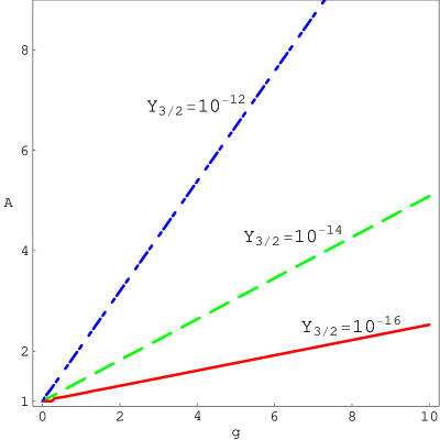
Figure 2: The gravitino yield in the inverted hybrid inflation model is plotted. The (red) solid line denote $Y_{3/2}=10^{-16}$, (green) dashed line $Y_{3/2}=10^{-14}$ and (blue) dash-dotted line $Y_{3/2}=10^{-12}$. In all the parameter region of this figure, the WMAP observation is reproduced and the sufficient baryon asymmetry is produced.

4 Summary

The supersymmetric standard model is very attractive, since it can explain the large hierarchy and the observed dark matter density. However, it was discovered that the supersymmetric standard model is not consistent with most of the inflation models, if the SUSY breaking is mediated by Planck suppressed operators. Under these circumstances, we have searched for successful inflation models in this paper.

Examining the gravitino production processes (i), (ii), (iii) and (iv) in the gravity mediation scenario, we have found that successful inflation models must have sufficiently low hight of the potential, an appropriate reheating temperature, and a small mass and a small VEV of the inflaton at the true vacuum. Studying these requirements and the WMAP results, we have found that a particular inverted hybrid inflation model is an example of such successful inflation models. Furthermore, we have found that this inflation model accommodates the see-saw mechanism and produces a sufficient baryon asymmetry by the leptogenesis mechanism. We consider that appropriate inflation models including this inverted hybrid inflation model will become interesting, when the gravity mediation scenario is confirmed in the future accelerator experiments.

References

• [1] A. H. Guth, Phys. Rev.  D 23, 347 (1981); A. D. Linde, Phys. Lett.  B 108, 389 (1982); A. Albrecht and P. J. Steinhardt, Phys. Rev. Lett.  48, 1220 (1982).
• [2] D. N. Spergel et al. [WMAP Collaboration], arXiv:astro-ph/0603449.
• [3] M. Kawasaki, F. Takahashi and T. T. Yanagida, Phys. Lett.  B 638, 8 (2006) [arXiv:hep-ph/0603265]; Phys. Rev.  D 74, 043519 (2006) [arXiv:hep-ph/0605297]; T. Asaka, S. Nakamura and M. Yamaguchi, Phys. Rev.  D 74, 023520 (2006) [arXiv:hep-ph/0604132].
• [4] M. Ibe, Y. Shinbara and T. T. Yanagida, Phys. Lett.  B 639, 534 (2006) [arXiv:hep-ph/0605252].
• [5] M. Endo, F. Takahashi and T. T. Yanagida, arXiv:0706.0986 [hep-ph].
• [6] M. Endo, M. Kawasaki, F. Takahashi and T. T. Yanagida, Phys. Lett.  B 642, 518 (2006) [arXiv:hep-ph/0607170].
• [7] M. Endo, F. Takahashi and T. T. Yanagida, arXiv:hep-ph/0701042.
• [8] M. Ibe and Y. Shinbara, arXiv:0710.1883 [hep-ph].
• [9] M. Endo, F. Takahashi and T. T. Yanagida, arXiv:hep-ph/0702247.
• [10] D. H. Lyth and E. D. Stewart, Phys. Rev.  D 54, 7186 (1996) [arXiv:hep-ph/9606412].
• [11] T. Banks, D. B. Kaplan and A. E. Nelson, Phys. Rev.  D 49, 779 (1994) [arXiv:hep-ph/9308292]; G. D. Coughlan, W. Fischler, E. W. Kolb, S. Raby and G. G. Ross, Phys. Lett.  B 131, 59 (1983); B. de Carlos, J. A. Casas, F. Quevedo and E. Roulet, Phys. Lett.  B 318, 447 (1993) [arXiv:hep-ph/9308325].
• [12] S. Nakamura and M. Yamaguchi, arXiv:0707.4538 [hep-ph].
• [13] K. I. Izawa and T. Yanagida, Prog. Theor. Phys.  95 (1996) 829 [arXiv:hep-th/9602180].
• [14] K. A. Intriligator and S. D. Thomas, Nucl. Phys.  B 473, 121 (1996) [arXiv:hep-th/9603158].
• [15] M. Kawasaki, K. Kohri and T. Moroi, Phys. Lett.  B 625, 7 (2005) [arXiv:astro-ph/0402490]. Phys. Rev.  D 71, 083502 (2005) [arXiv:astro-ph/0408426].
• [16] K. Kohri, T. Moroi and A. Yotsuyanagi, Phys. Rev.  D 73 (2006) 123511 [arXiv:hep-ph/0507245].
• [17] H. Murayama, H. Suzuki, T. Yanagida and J. Yokoyama, Phys. Rev.  D 50 (1994) 2356 [arXiv:hep-ph/9311326].
• [18] M. Kawasaki, M. Yamaguchi and T. Yanagida, Phys. Rev. Lett.  85, 3572 (2000) [arXiv:hep-ph/0004243].
• [19] K. I. Izawa, M. Kawasaki and T. Yanagida, Prog. Theor. Phys.  101, 1129 (1999) [arXiv:hep-ph/9810537].
• [20] M. Kawasaki, N. Sakai, M. Yamaguchi and T. Yanagida, Phys. Rev.  D 62, 123507 (2000) [arXiv:hep-ph/0005073].
• [21] M. Kawasaki and M. Yamaguchi, Phys. Rev.  D 65, 103518 (2002) [arXiv:hep-ph/0112093].
• [22] G. R. Dvali, Q. Shafi and R. K. Schaefer, Phys. Rev. Lett.  73, 1886 (1994) [arXiv:hep-ph/9406319].
• [23] E. D. Stewart, Phys. Lett.  B 345, 414 (1995) [arXiv:astro-ph/9407040].
• [24] G. Lazarides and C. Panagiotakopoulos, Phys. Rev.  D 52, 559 (1995) [arXiv:hep-ph/9506325].
• [25] A. D. Linde and A. Riotto, Phys. Rev.  D 56, 1841 (1997) [arXiv:hep-ph/9703209].
• [26] K. I. Izawa and T. Yanagida, Phys. Lett.  B 393, 331 (1997) [arXiv:hep-ph/9608359]; T. Asaka, K. Hamaguchi, M. Kawasaki and T. Yanagida, Phys. Rev.  D 61, 083512 (2000) [arXiv:hep-ph/9907559]; V. N. Senoguz and Q. Shafi, Phys. Lett.  B 596, 8 (2004) [arXiv:hep-ph/0403294].
• [27] M. Endo, K. Hamaguchi and F. Takahashi, Phys. Rev. Lett.  96, 211301 (2006) [arXiv:hep-ph/0602061]; S. Nakamura and M. Yamaguchi, Phys. Lett.  B 638, 389 (2006) [arXiv:hep-ph/0602081].
• [28] M. Endo, K. Hamaguchi and F. Takahashi, Phys. Rev.  D 74, 023531 (2006) [arXiv:hep-ph/0605091].
• [29] S. Weinberg, Phys. Rev. Lett.  48, 1303 (1982); L. M. Krauss, Nucl. Phys.  B 227, 556 (1983).
• [30] L. Alabidi and D. H. Lyth, JCAP 0608, 013 (2006) [arXiv:astro-ph/0603539].
• [31] T. Yanagida, in Proc. Workshop on the Unified Theory and Baryon Number in the Universe, ed. by O. Sawada, A. Sugamoto (KEK report 79-18, 1979), p. 95; M. Gell-Mann, P. Ramond, R. Slansky, in Supergravity, ed. by P. van Nieuwenhuizen, D.Z. Freedman (North Holland, Amsterdam 1979), p. 315.
• [32] For a review, D. H. Lyth and A. Riotto, Phys. Rept.  314, 1 (1999) [arXiv:hep-ph/9807278]; L. Alabidi and D. H. Lyth, JCAP 0605, 016 (2006) [arXiv:astro-ph/0510441].
• [33] M. Fukugita and T. Yanagida, Phys. Lett.  B 174, 45 (1986);
For a review, W. Buchmuller, R. D. Peccei and T. Yanagida, Ann. Rev. Nucl. Part. Sci.  55, 311 (2005) [arXiv:hep-ph/0502169].
• [34] D. H. Lyth, JCAP 0704, 006 (2007) [arXiv:hep-ph/0605283].