Probing Non-Gaussianity In The Cosmic Microwave Background Anisotropies: One Point Distribution Function

Abstract

We analyze WMAP 3 year data using the one-point distribution functions to probe the non-Gaussianity in the Cosmic Microwave Background (CMB) Anisotropy data. Computer simulations are performed to determine the uncertainties of the results. We report the non-Gaussianity parameter $f_{\mathrm{NL}}$ is constrained to $26<f_{\mathrm{NL}}<82$ for Q-band, $12<f_{\mathrm{NL}}<67$ for V-band, $7<f_{\mathrm{NL}}<64$ for W-band and $23<f_{\mathrm{NL}}<75$ for Q+V+W combined data at 95% confidence level (CL).

I introduction

Non-Gaussianity is one of the most important tests of models of the inflation. Among the various theoretical models on the inflation, slow-roll inflation is currently most lively being studied. There are various predictions on the magnitude of non-Gaussianity based on the simple model of slow-roll inflation and its extensions, ranging from undetectably tiny values to large enough values to be detectable with currently available data Barnaby and Cline (2007); Battefeld and Easther (2007); Calcagni (2005); Creminelli (2005); Bartolo et al. (2002). On the other hand, observational works have claimed both detection and non-detection of non-Gaussianity (for reviews on recent works, see Komatsu et al. (2003); Spergel et al. (2007); Troia et al. (2007); Creminelli et al. (2007); Gaztanaga and Wagg (2003)). Among the popular techniques for detecting non-Gaussianity are one-point distribution function fitting, bispectrum, trispectrum and Minkowski functionals. Here, we investigate the one-point distribution functions to probe primordial non-Gaussianity in the CMB anisotropy data. An observed CMB anisotropy at a direction ($\delta T_{obs}$) can be regarded as the superposition of three parts: physical fluctuation of cosmic origin ($\delta T_{p}$), instrumental noise ($\delta T_{n}$), and foreground emissions ($T_{fg}$). Since the foreground templates are separately prepared, we start with foreground-removed data of which the CMB anisotropy can be decomposed into two uncorrelated components,

$$\delta T=\delta T_{obs}-T_{fg}=\delta T_{p}+\delta T_{n}.$$ (1)

The primary source for the cosmic fluctuation of CMB at the large scale is attributed to the Sachs-Wolfe effect which is again triggered by the primordial curvature perturbation. The curvature perturbation $\Phi$ by primordial seed during the inflation is transferred to CMB anisotropy with the relation

$$\frac{\delta T_{p}\left({\bf{x}}\right)}{T_{0}}=\eta_{t}\Phi\left({\bf{x}}\right)$$ (2)

where $T_{0}=2.725$ K, the thermodynamic temperature of the CMB today, and $\eta_{t}$ is the radiation transfer function. For the super-horizon scale, we take $\eta_{t}=-1/3$ from the Sachs-Wolfe effects. At the first-order of perturbation, we may replace $\Phi=\Phi_{g}$, where $\Phi_{g}$ is an auxiliary random Gaussian field with its mean $\langle\Phi_{g}\rangle=0$ and its variance denoted by $\langle\Phi_{g}^{2}\rangle$. When the second-order perturbation is considered, it is conventional to prescribe the nonlinear coupling of the curvature perturbation as Komatsu and Spergel (2001)

$$\Phi({\bf{x}})\simeq\Phi_{g}({\bf{x}})+f_{\mathrm{NL}}\left(\Phi_{g}^{2}({\bf{x}})-\langle\Phi_{g}^{2}\rangle\right)$$ (3)

where $f_{\mathrm{NL}}$ is the non-Gaussianity parameter. The second term in (3) is responsible for the non-Gaussianity of the primordial fluctuation. Then, the probability distribution function of the non-Gaussian field $\Phi$ can be derived as

$$f_{\Phi}(\Phi) = \int f_{G}(\Phi_{g})\delta_{D}\left[\Phi-\Phi_{g}-f_{\mathrm{NL}}\left(\Phi_{g}^{2}-\langle\Phi_{g}^{2}\rangle\right)\right]d\Phi_{g}$$ (4)

$$= \frac{1}{\sqrt{2\pi\langle\Phi_{g}^{2}\rangle f_{\mathrm{NL}}^{2}\left(\Phi_{+}-\Phi_{-}\right)^{2}}}$$

$$\times\left[\exp\left(-\frac{\Phi_{+}^{2}}{2\langle\Phi_{g}^{2}\rangle}\right)+\exp\left(-\frac{\Phi_{-}^{2}}{2\langle\Phi_{g}^{2}\rangle}\right)\right]$$

where $\Phi_{\pm}$ are defined by

$$\Phi_{\pm}=\frac{1}{2f_{\mathrm{NL}}}\left[-1\pm\sqrt{1+4f_{\mathrm{NL}}\Phi+4f_{\mathrm{NL}}^{2}\langle\Phi_{g}^{2}\rangle}\right]$$ (5)

and $\Phi$ has to be limited by the reality of $\Phi_{\pm}$ as

$$f_{\mathrm{NL}}\Phi>-\frac{1}{4}-f_{\mathrm{NL}}^{2}\langle\Phi_{g}^{2}\rangle.$$ (6)

$\langle\Phi_{g}^{2}\rangle$ can be expressed in terms of $\eta_{t}$, $T_{0}$ and $\sigma_{CMB}$,

$$\langle\Phi_{g}^{2}\rangle=\frac{1}{4f_{\mathrm{NL}}^{2}}\left[-1+\sqrt{1+8\left(\frac{f_{\mathrm{NL}}\sigma_{CMB}}{\eta_{t}T_{0}}\right)^{2}}\right].$$ (7)

For a pixelized CMB anisotropy data set, the probability distribution function for Gaussian instrumental noise becomes

$$f_{N}(\delta T_{n})=\frac{1}{N_{pix}}\sum_{i=1}^{N_{pix}}\frac{1}{\sqrt{2\pi\sigma_{0}^{2}/n_{i}}}\exp\left[-\frac{\delta T_{n}^{2}}{2\sigma_{0}^{2}/n_{i}}\right]$$ (8)

where $n_{i}$ is the effective number of measurements at the $i_{th}$ pixel and $\sigma_{0}$ represents the dispersion of the instrumental noise per observation ($\sigma_{0}$=2.1898, 3.1249, 6.5112 mK for Q, V, W-band, respectively Limon et al. (2006)). Now, it is straightforward to express the probability density function for $\delta T$ in an integral form,

$$f(\delta T) = \int f_{\delta T_{p}}(\delta T_{p})f_{N}(\delta T_{n})$$ (9)

$$\times\delta_{D}\left(\delta T-\delta T_{p}-\delta T_{n}\right)d\delta T_{p}d\delta T_{n}$$

$$= \int f_{\Phi}(\Phi)f_{N}(\delta T_{n})$$

$$\times\delta_{D}\left(\delta T-\eta_{t}T_{0}\Phi-\delta T_{n}\right)d\Phi d\delta T_{n}.$$

The probability density function derived in (9) explicitly contains the non-Gaussianity parameter $f_{\mathrm{NL}}$, and it can serve as the prediction of one-point distribution function with a given $f_{\mathrm{NL}}$ for a (ideally) foreground-removed CMB anisotropy data set to estimate the magnitude of deviation from Gaussian distribution in a quantitative manner.

II Application to WMAP data

We use the three channels of WMAP 3 year CMB anisotropy data sets (Q (33GHz)-, V (61GHz)-, W (94GHz)-band) which contain dominant signal over contaminations to investigate the non-Gaussianity of the CMB anisotropy data. To remove the foreground emissions, the Maximum Entropy Method (MEM) maps of the synchrotron, free-free and thermal dust are used. The Kp0-mask is applied to the sky maps to remove the intense Galactic emissions and scattered bright point sources, which leaves 76.5% of the sky. We also prepare a combined map (Q+V+W) by taking a weighted sum for a pixel temperature,

$$\delta T\left({\bf{x}}\right)=\frac{\sum_{i}\delta T_{i}\left({\bf{x}}\right)n_{i}\left({\bf{x}}\right)/\sigma_{0i}^{2}}{\sum_{i}n_{i}\left({\bf{x}}\right)/\sigma_{0i}^{2}},\quad i={\mathrm{Q,\>V,\>W}}$$ (10)

where $n_{i}\left({\bf{x}}\right)$ is the effective number of measurements at the pixelized position ${\bf{x}}$ and $\sigma_{0i}$ is the dispersion of the instrumental noise of the $i_{\mathrm{th}}$ channel. We can trace the effective variance of the instrumental noise as a result of weighted sum defined in (10) as

$$\sigma^{2}\left({\bf{x}}\right)=\left[\sum_{i}n_{i}\left({\bf{x}}\right)/\sigma_{0i}^{2}\right]^{-1},\quad i={\mathrm{Q,\>V,\>W}}.$$ (11)

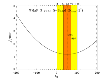
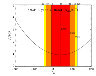
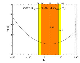
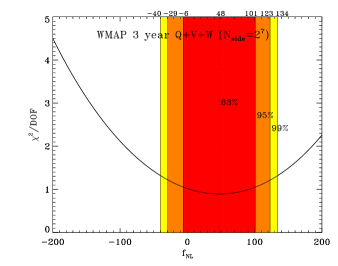
The sky map data are degraded from $N_{\mathrm{side}}=512$ ($6.87^{\prime}$ pixel) to $N_{\mathrm{side}}=128$ ($27.48^{\prime}$ pixel) where the number of pixels in a full sky map is given by $12\times N_{\mathrm{side}}^{2}$. The purpose of demotion of the resolution is to suppress the small scale fluctuation which is dominated by the instrumental noise. We perform the $\chi^{2}$-test for the goodness of fit for the probability density function given in (9) as a prediction to the observed probability density function which is directly calculated from the WMAP data. Figure 1 and Table 1 show the results of $\chi^{2}$ fitting of WMAP data sets with varying $f_{\mathrm{NL}}$ as a free parameter. All data sets are best fitted at positive $f_{\mathrm{NL}}$ (dubbed $f_{\mathrm{NL}}^{\left(\mathrm{opt}\right)}$) which are consistent with one another as well as the results with previous work Spergel et al. (2007) within the statistical errors.

Figure 1: $\chi^{2}$-test for goodness of fit is used to find the optimal value of the non-Gaussianity parameter. The anisotropy maps are demoted to $N_{{\mathrm{side}}}=2^{7}$. Top left: Q-band, top right: V-band, bottom left: W-band, bottom right: Q+V+W combined. The color (shaded) bands indicate the bounds on $f_{\mathrm{NL}}$ in which the probability that the statistic $\chi^{2}$ is smaller than that of the observed with respect to the prediction curve with $f_{\mathrm{NL}}$.

Map	Q-band		V-band		W-band		Q+V+W
$f_{\mathrm{NL}}^{\left(\mathrm{opt}\right)}$	53		39		35		48
68%	N/A		-9$<\!f_{\mathrm{NL}}\!<$	86	N/A		-6$<\!f_{\mathrm{NL}}\!<$	101
95%	34$<\!f_{\mathrm{NL}}\!<$	71	-37$<\!f_{\mathrm{NL}}\!<$	113	-20$<\!f_{\mathrm{NL}}\!<$	89	-29$<\!f_{\mathrm{NL}}\!<$	123
99%	3$<\!f_{\mathrm{NL}}\!<$	102	-49$<\!f_{\mathrm{NL}}\!<$	126	-37$<\!f_{\mathrm{NL}}\!<$	106	-40$<\!f_{\mathrm{NL}}\!<$	134
DOF	119		119		119		119

Table 1: The results of $\chi^{2}$-tests for Goodness-of-fit for WMAP 3 year data. The percentages on the first column represent the tail probabilities at which the statistic $\chi^{2}$ would be smaller than the observed. DOF on the bottom row stands for Degrees of freedom.

III Simulation And Statistical Uncertainties

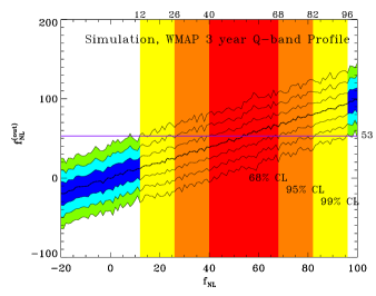
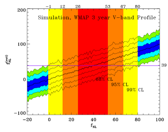
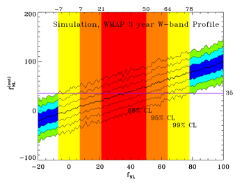
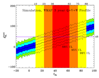
As is shown in Figure 1, WMAP data fit well with finite range of the non-Gaussianity parameter $f_{\mathrm{NL}}$. We pick $f_{\mathrm{NL}}^{\left(\mathrm{opt}\right)}$ as the representative magnitude of non-Gaussianity for a data set, and carry out the Monte-Carlo simulations to test the pertinence of $f_{\mathrm{NL}}^{\left(\mathrm{opt}\right)}$ as a proper measure of non-Gaussianity for a data set in a quantitative manner. A simulated data set is prepared as follows: First, a Gaussian field $\Phi_{g}$ with its variance equal to (7) is generated and we use it to generate $\Phi$-field of which the deviation from Gaussianity is denoted by $f_{\mathrm{NL}}$. Second, we prepare a noise map in which each pixel contains a random value picked from a normal distribution with variance $\sigma_{0}^{2}/n_{i}$ as defined in (8) and add this to $\Phi$-field. A simulated map generated in this way has the same noise structure and the dispersion of physical fluctuation ($\sigma_{CMB}$) as a real data set. Since a data set contains nontrivial instrumental noise and the number of pixels is finite, the returned magnitude of non-Gaussianity ($f_{\mathrm{NL}}^{\left(\mathrm{opt}\right)}$) would have some uncertainty. For a given value of $f_{\mathrm{NL}}$, we repeat the simulation and find that the algorithm returned an unbiased, normal distribution of $f_{\mathrm{NL}}^{\left(\mathrm{opt}\right)}$ which is centered at the input value of $f_{\mathrm{NL}}$. Thus, from the results of the simulations, we are able to set the bounds on $f_{\mathrm{NL}}$ for the real data. The simulation results and error bands are plotted in Figure 2 and the deduced uncertainties for $f_{\mathrm{NL}}$ are summarized in Table 2. It is very remarkable that this analysis strongly disfavors the null hypothesis ($f_{\mathrm{NL}}=0$) and all the data sets show consistent results within the statistical errors. The results are also consistent with the works by the WMAP team ($-54<f_{\mathrm{NL}}<114$ at 95% CL from bispectrum Spergel et al. (2007)) but with much tighter limits and more importantly, it excludes $f_{\mathrm{NL}}=0$ at 95% CL.

Figure 2: Error bands found through the simulations with the same profiles with WMAP 3 year data (blue-green slanted bands). Here the “same profile” means that the simulated data set has exactly same instrumental noise structure and $\sigma_{CMB}$ as a real WMAP data set has. The vertical bands indicate the bounds for $f_{\mathrm{NL}}^{\left(\mathrm{opt}\right)}$ found from the analysis of the WMAP data. Top left: Q-band, top right: V-band, bottom left: W-band, bottom right: Q+V+W. On the vertical axis, $f_{\mathrm{NL}}^{\left(\mathrm{out}\right)}$ is the measured $f_{\mathrm{NL}}^{\left(\mathrm{opt}\right)}$ from the simulated data.

Map	Q-band		V-band		W-band		Q+V+W
$N_{\mathrm{sim}}$	100		100		100		100
68%	40$<f_{\mathrm{NL}}<$	68	26$<f_{\mathrm{NL}}<$	53	21$<f_{\mathrm{NL}}<$	50	36$<f_{\mathrm{NL}}<$	62
95%	26$<f_{\mathrm{NL}}<$	82	12$<f_{\mathrm{NL}}<$	67	7$<f_{\mathrm{NL}}<$	64	23$<f_{\mathrm{NL}}<$	75
99%	12$<f_{\mathrm{NL}}<$	96	-1$<f_{\mathrm{NL}}<$	80	-7$<f_{\mathrm{NL}}<$	78	9$<f_{\mathrm{NL}}<$	88

Table 2: Summary of results from Simulations with WMAP 3 year data profiles and the bounds at three confidence levels from the simulations.

IV Conclusion

We developed an algorithm that uses the one-point distribution function to investigate the non-Gaussianity of CMB anisotropy data, and applied it to WMAP 3 year data. We found that the null result ($f_{\mathrm{NL}}$=0) is manifestly excluded at 95% CL. The estimated magnitude of non-Gaussianity parameter is $23<f_{\mathrm{NL}}<75$ at 95% CL and $9<f_{\mathrm{NL}}<88$ at 99% CL for the (Q+V+W)-combined map. Since the quadratic term in (3) takes a generic form of Taylor series for a perturbative expansion, it is a good possibility that the observed non-Gaussianity in this work is a combined effects of various physical processes, while the primordial seeds are very likely to be the leading one. There are two premises we have taken in developing the algorithm, which, provided they are not precise enough, could cause non-Gaussianity of not cosmic but systematic origin: (1) the probability distribution function of the instrumental noise for each pixel is centered at zero, and (2) the foreground emissions are removed efficiently enough in the foreground-removed maps. The first condition can be broken when the thermal and radiation environments of the WMAP satellite in its orbit are taken into account, while the WMAP team assessed they are insufficient to influence the science data Limon et al. (2006). So, we tested the effects of the alternative noise distributions with a random mean in each of the Gaussian distribution in (8) and the algorithm was not misled to show non-Gaussianity within the statistical error. It is difficult to directly estimate how much residual foreground emissions after foreground subtraction would affect the one-point distribution function. We solely rely on the quality of foreground templates and it is remarkably successful, showing that the observed total Galactic emission matches the model to less than 1% Bennett et al. (2003); Hinshaw et al. (2007). We also analyzed simulated maps which are (Gaussian map + foreground templates), and all the templates for Q, V and W-channel showed negative values of the non-Gaussianity parameter with $\left|f_{\mathrm{NL}}\right|\sim\mathcal{O}\left(10^{1}\right)$ at the resolution $N_{\mathrm{side}}=512$.