The Chandra Small Magellanic Cloud Wing Survey - the search for X-ray Binaries

Abstract

We have detected 523 sources in a survey of the Small Magellanic Cloud (SMC) Wing with Chandra. By cross-correlating the X-ray data with optical and near-infrared catalogues we have found 300 matches. Using a technique that combines X-ray colours and X-ray to optical flux ratios we have been able to assign preliminary classifications to 265 of the objects. Our identifications include four pulsars, one high-mass X-ray binary (HMXB) candidate, 34 stars and 185 active galactic nuclei (AGNs). In addition, we have classified 32 sources as ’hard’ AGNs which are likely absorbed by local gas and dust, and nine ’soft’ AGNs whose nature is still unclear. Considering the abundance of HMXBs discovered so far in the Bar of the SMC the number that we have detected in the Wing is low.

1 Introduction

Multi-wavelength studies of the Small Magellanic Cloud (SMC) have shown that it contains a large number of X-ray binary pulsars. From analysis of H$\alpha$ measurements (Kennicutt, 1991) and supernova birth rates (Filipovic et al., 1998) the star formation rate (SFR) for the SMC is estimated to lie in the range 0.04–0.4 $M_{\odot}$ yr^-1. Shtykovskiy & Gilfanov (2005) used these upper and lower SFR estimates and the linear relation between the number of high-mass X-ray binaries (HMXBs) and the SFR of the host galaxy from Grimm, Gilfanov & Sunyaev (2003) to predict the number of HMXBs expected in the SMC with luminosities $\geq 10^{35}$ erg s^-1. They found that between 6 and 49 of these systems should be present. Currently $\sim 60$ known or probable HMXBs have been detected in the SMC (see e.g. Haberl & Pietsch, 2004; Coe et al., 2005; McGowan et al., 2007).

It is believed that the considerable number of pulsars can be explained in terms of a dramatic phase of star formation, probably related to the most recent closest approach of the SMC and the Large Magellanic Cloud (LMC; Gardiner & Noguchi, 1996). To date most of the X-ray studies of the SMC have concentrated on the Bar which has proved to be a significant source of HMXBs. These systems not only provide an homogeneous sample for study, but also give direct insights into the history of our neighbouring galaxy as they are tracers of star formation rates.

Part of the puzzle of the X-ray population of the SMC is the missing or under represented components. In particular, there are no known low-mass X-ray binaries (LMXBs) or black hole binaries and only one confirmed supergiant X-ray binary detected to date (see also McBride et al., 2007a). A survey of the X-ray binary population of the LMC by Negueruela & Coe (2002) revealed a similar distribution (within small number statistics) to that in our galaxy - all types were present. It is therefore important to try and identify the “missing” X-ray binary types in the SMC.

We recently completed the first X-ray survey in the SMC Wing with Chandra (see Section 2 for more details). A study of the brightest ($>50$ counts) X-ray sources uncovered two new pulsars, and detected two previously known pulsars (McGowan et al., 2007). In addition to the four pulsars, the sample included two foreground stars, 12 probable AGNs and five unclassified sources. We found that the pulsars had harder spectra than the other bright X-ray sources. In this paper we report on the analysis of the whole survey and present preliminary classifications for a large fraction of the sources detected.

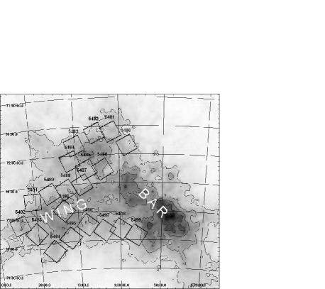
Figure 1: The location of the 20 fields studied by Chandra in this work, overlaid on a neutral hydrogen density image of the SMC (Stanimirović et al., 1999). The Wing and Bar of the SMC are marked.

2 Observations and Data Analysis

Coe et al. (2005) studied the locations of known X-ray pulsars in the SMC Bar and believed they identified a relationship between the HI intensity distribution and that of the pulsars. They found that the pulsars seem to lie in regions of low/medium HI densities, suggesting that high-mass star formation is well suited to these densities. Based on these results observations in the Wing of the SMC were made from 2005 July to 2006 March with Chandra (see Figure 1). The survey consisted of 20 fields, with exposure times ranging from 8.6–10.3 ks. The observation log is presented in Table 1. The measurements were performed with the standard ACIS-I (Garmire et al., 2003) imaging mode configuration which utilises chips I0-I3 plus S2 and S3.

The data were processed using CIAO V3.3. We filtered the event files to restrict the energy range to 0.5–8.0 keV. Exposure maps for each field were generated assuming an absorbed power-law distribution of source photons with index of 1.6 and neutral hydrogen column density of $6\times 10^{20}$ cm^-2 (Dickey & Lockman, 1990). A large number of the sources are background active galactic nuclei (AGNs; see Section 7). The photon index was chosen based on the spectral fitting results for the brightest X-ray sources in the survey from McGowan et al. (2007).

2.1 Source detection

We searched for sources using the WAVDETECT tool. The detection algorithm was run on each field using the appropriate exposure map, wavelet scales of 1.0, 2.0, 4.0, 8.0 and 16.0 pixels, where a pixel is $0\aas@@fstack{\prime\prime}49$ square, and a significance threshold of $10^{-7}$. The initial wavelet scale size is chosen to match the point-spread function (PSF), which has an on-axis FWHM of $\sim 0\aas@@fstack{\prime\prime}5$. The size of the PSF is heavily dependent on the off-axis angle, increasing to $\sim 2\aas@@fstack{\prime\prime}0$ at $\sim 6\aas@@fstack{\prime}0$ off-axis. The choice of significance threshold should yield $\sim 1$ false detection over a $2048\times 2048$ pixel image. Hornschemeier et al. (2001) have shown that in general the counts detected using wavelet analysis agree well with the counts determined from aperture photometry. We converted the observed count rates to source fluxes by employing the same absorbed power-law spectrum as above.

Figure 2: Distribution of net counts for the sources detected in the SMC Wing survey.

3 The SMC Wing Survey Catalogue

A total of 523 sources have been detected in the 20 fields. The number of sources detected in each field varies from 16–36 (see Table 1), with the measured counts per source ranging from 2–1918, with a median of 8 counts. The distribution of counts is shown in Figure 2. A sample of the catalogue is presented in Table 2 (the full catalogue is available as Supplementary Material in the electronic edition of the journal). The columns in the table are as follows, the catalogue source number, the right ascension and declination taken from the wavelet analysis, the error on the source position (see below), the net counts which are the total source counts (background subtracted) in the 0.5–8 keV energy band, the signal-to-noise of the detection given by the wavelet algorithm, the source flux which was determined by converting the observed count rate to a flux employing the absorbed power-law spectrum from Section 2, the median, compressed median and normalised quartile ratio quantile values (see Section 4), the $V$- and $R$-band magnitudes and the $B-V$ colour of the optical counterpart (see Section 5), X-ray to optical flux ratios based on the $V$- and $R$-band magnitudes, respectively (see Section 6), and the preliminary classification for the source (see Section 7).

The significance threshold chosen for our analysis ($10^{-7}$) indicates that we should detect $\sim 1$ spurious source per field, giving a total of $\sim 20$ spurious sources in our catalogue. We find 17 sources with a signal-to-noise of $\leq 1.5$ (each has 2–3 net counts) which could be false detections. For completeness, we have included these potentially spurious sources in the catalogue.

The errors on the source positions were calculated by taking into account the properties of the telescope optics and the source brightness (see Hong et al., 2005). The positional error given in the catalogue is the 95% confidence region, combined in quadrature with the boresight error ($\sim 0.7\arcsec$ at 95% confidence).

The median count value, converted to a rate, corresponds roughly to a flux of $9\times 10^{-15}$ erg cm^-2 s^-1. At a distance to the SMC of 60 kpc (based on the distance modulus, Westerlund, 1997) this flux corresponds to a luminosity of $\sim 3.9\times 10^{33}$ erg s^-1. This limit is adequate to detect fainter HMXBs and active LMXBs, but is insufficient for quiescent LMXBs which can be as faint as $2\times 10^{30}$ erg s^-1 (Garcia et al., 2001).

4 Quantile Analysis

We have used the quantile analysis technique of Hong et al. (2004) to investigate the X-ray colours of the sources detected in our survey. In a traditional hardness ratio the photons are split into predefined energy bands. The quantile method divides the photon distribution into a given number of equal proportions, where the quantiles are the energy values that mark the boundaries between consecutive subsets. This has the advantage, compared to traditional hardness ratios, that there is no spectral dependence and a colour can be calculated even for sources with very few counts (for more details see Hong et al., 2004).

For each source that has $\geq 3$ counts we determine the median and quartiles of the photon energy distribution, including background subtraction. We list in Table 2 the median ($m=Q_{50}$), a compressed median given by $\log_{10}(m/1-m)$ and a normalised quartile ratio of $3(Q_{25}/Q_{75})$. Using the compressed median and the quartile ratio we can construct quantile-based colour-colour diagrams (QCCDs). By generating a quantile-based colour-colour diagram McGowan et al. (2007) were able to investigate the properties of the 23 X-ray brightest survey sources. It was found that the four pulsars detected in the SMC Wing Survey lay in a distinct (hard) region on the QCCD.

Table 1: Observation Log

Obs	Date	Central	Central	Exp	No. of
ID		RA	Dec.		Sources
		(J2000)	(J2000)	(ks)
5480	2006-02-06	00:58:20	-71:50:27	9.59	16
5481	2006-02-06	01:01:54	-71:35:58	9.34	31
5482	2006-02-06	01:05:31	-71:37:06	9.34	25
5483	2006-02-06	01:10:10	-71:49:29	9.34	19
5484	2006-02-06	01:11:20	-72:05:38	9.52	30
5485	2006-02-08	01:07:41	-72:14:54	10.05	25
5486	2006-02-10	01:03:53	-72:15:06	9.83	28
5487	2006-02-10	01:08:47	-72:30:50	9.63	29
5488	2006-02-12	01:12:39	-72:35:17	10.02	36
5489	2006-02-12	01:16:35	-72:38:16	9.63	32
5490	2006-02-27	01:13:21	-72:57:10	10.32	25
5491	2005-07-24	01:20:36	-72:45:40	9.06	27
5492	2005-08-12	01:24:10	-73:09:02	10.06	26
5493	2006-02-27	01:20:28	-73:19:27	9.68	23
5494	2006-03-01	01:16:21	-73:38:54	9.91	32
5495	2006-03-01	01:12:09	-73:26:10	9.63	18
5496	2006-03-03	01:07:55	-73:13:10	9.82	24
5497	2006-03-03	01:03:53	-73:19:33	8.64	22
5498	2006-03-03	00:59:59	-73:18:34	9.63	29
5499	2006-03-03	00:56:10	-73:25:15	9.64	26

Figure 3: The number of matches as a function of search radius between the optical/near-infrared catalogues (for a list see Section 5) and the SMC Wing X-ray positions (filled squares). We also show the results of correlating the simulated positions (see text for details) with the optical/near-infrared catalogues (triangles). The difference between the number of real and simulated matches is also plotted (solid line).

5 Optical Identifications

To search for possible optical counterparts for our Chandra sources we cross-correlated the X-ray positions with the following catalogues: Magellanic Clouds Photometric Survey: the SMC (Zaritsky et al., 2002), Guide Star Catalog, v.2.2.1 (Morrison & McLean, 2001), The CCD Survey of the Magellanic Clouds (Massey, 2002), USNO-B1.0 Catalog (Monet et al., 2003), the MACHO online database and The 2MASS All-Sky Catalog of Point Sources (Cutri et al., 2003). We chose the search radius based on a comparison of a correlation of the real X-ray positions with the optical/near-infrared catalogues with a correlation of simulated positions with the catalogues, both over a range of search radii (see e.g. Barlow et al., 2006). Only the nearest optical match was taken in each case. The correlations were performed using all of the catalogues given above apart from the MACHO catalogue, as it was not possible to automate that search. The simulated positions were generated by mirroring the source declinations around an arbitrary declination in the SMC. This method was chosen to try and ensure that the simulated positions lie in similar density regions in the SMC as the real positions.

The results of the correlations are shown in Figure 3. The difference between the number of real and simulated matches is also plotted. The value at which the number of real matches is still increasing more rapidly than those from the simulated data can be considered as the optimum search radius. Our figure indicates that a radius of $\leq 2\arcsec$ should be used, after which the number of real and simulated matches grow at the same rate. We have therefore used a search radius of $2\arcsec$ in our cross-correlations, giving us an estimate of the expected number of false matches of 33%. We note that the choice of search radius is a trade-off between one that is too small and gives a very conservative number of matches and one that is too large leading to many spurious matches. In our case we find that for four of our sources, all stars, a radius of $2\arcsec$ is too small and a larger radius of $3\arcsec$ must be used to obtain a likely match.

Our calculations of the errors on the source positions (see Section 3) show that 288 of our sources have uncertainties of $\leq 2\arcsec$, implying that the chosen search radius is adequate for more than half (55%) of the objects in our survey. There are 72 sources which have a positional error of $\leq 1\arcsec$. For these sources, if the position of the nearest optical match differed greatly from the X-ray position we checked the match by eye to confirm a likely counterpart.

Out of 523 X-ray sources we find 300 optical and/or near-infrared matches within the chosen search radius. The number of matches shown in Figure 3 is less than this as the matches to the MACHO catalogue are not included. The majority of the fields have a match success of 39–90%, with a median of 67%. However, there are three fields 5491, 5492 and 5493 on the Eastern edge of the Wing of the SMC (see Figure 1) which have very sparse coverage in the optical and near-infrared, resulting in only 19–26% of the sources in those fields being matched.

6 X-ray to Optical Flux Ratios

We have calculated X-ray to optical flux ratios for the sources in our survey that have optical matches. It has been shown that such ratios are a good discriminator for different classes of objects (see e.g. Maccacaro et al., 1988; Hornschemeier et al., 2001; Shtykovskiy & Gilfanov, 2005). We have employed two of these kinds of ratio, one based on the $V$ magnitude and the other on the $R$ magnitude of the source. The former ratio, from Shtykovskiy & Gilfanov (2005), is useful for distinguishing between HMXBs and stars in the magnitude range $12<V<18$. In this case stars are identified as sources that have $B-V>0.6$ and $f_{\rm X_{\rm H}}/f_{V}<10^{-3}$, where $f_{V}=8.0\times 10^{-6}\cdot 10^{-m_{V}/2.5}$ erg s^-1 cm^-2, and $f_{\rm X_{\rm H}}$ is the flux in the 2–10 keV energy band. The latter ratio can be used to classify AGNs, with typical values for these sources lying in the region $\log(f_{\rm X_{\rm S}}/f_{R})=0.0\pm 1.0$, where $f_{\rm X_{\rm S}}$ is the flux in the 0.5–2 keV range and $\log(f_{\rm X_{\rm S}}/f_{R})=\log f_{\rm X_{\rm S}}+5.50+R/2.5$ (Hornschemeier et al., 2001). Given the measured flux for our sources in the 0.5–8 keV energy range we determined the flux in the 0.5–2 keV and 2–10 keV bands using PIMMS v3.9a, assuming the same absorbed power-law spectrum from Section 2.

7 Source Classification

The X-ray to optical flux ratios, combined with the quantile results, allow us to provisionally classify the sources in the SMC Wing Survey.

7.1 Foreground stars

Using the X-ray to optical flux ratio and colour criteria from Shtykovskiy & Gilfanov (2005) we identified a number of stars in the SMC Wing survey. In addition, a few objects with magnitudes brighter than $V=12$ were also classified as stars. Applying this method we found 16 stars. These objects are most likely foreground stars exhibiting coronal X-ray emission. We note that the $f_{\rm X_{\rm H}}/f_{V}$ values for the sources we have placed in the star category range from $1.5\times 10^{-5}-0.03$ with a median value of 0.005. In the cases where $f_{\rm X_{\rm H}}/f_{V}>10^{-3}$ the classification was made based primarily on the magnitude and colours of the source. Six of the sources we have classified as stars have $f_{\rm X_{\rm H}}/f_{V}\geq 0.01$ and fall in the magnitude and colour ranges $V=14.3-17.9$ and $B-V=0.81-1.32$, respectively.

7.2 High-mass X-ray binaries

In Shtykovskiy & Gilfanov (2005) the authors investigated XMM-Newton observations of the SMC, mainly located in the Bar, with the purpose of determining HMXB candidates in the region surveyed. A total area of 1.48 deg² was covered with a flux limit of $\sim 10^{-14}$ erg s^-1 cm^-2 (which corresponds to a luminosity of $\sim 4.3\times 10^{33}$ erg s^-1 at the distance of the SMC). They cross-correlated the X-ray positions with optical and near-infrared catalogues using a search radius of $4\arcsec$. Any source that did not result in an optical match was discarded. To identify HMXBs they required that the magnitude of the optical counterpart lay in the range $12.0<V<18.0$ and the optical and/or infrared colours were $B-V<0.6$ and $J-K\la 0.1-0.2$, respectively. They also imposed a limit for the X-ray to optical flux ratio, with any source having $f_{\rm X_{\rm H}}/f_{V}<10^{-3}$ being rejected. Applying these criteria Shtykovskiy & Gilfanov (2005) found 32 likely HMXBs and 18 sources whose nature is uncertain.

Employing the same filters we find four of our sources satisfy the magnitude and optical colour criteria (catalogue sources 29, 91, 114 and 193); all of which have already been identified as Be X-ray pulsars (see McGowan et al., 2007; Schurch et al., 2007). Out of these four sources, only three have $J-K$ values. The $J-K$ colours for the pulsars are 0.1, 0.3 and 0.6, leading to two out of the three sources failing the Shtykovskiy & Gilfanov (2005) criteria. However, the $J-K$ colours of identified SMC Be X-ray binaries can be shown to lie in a much broader range of -0.2 – $>$0.7 (see e.g. Coe et al., 2005), which is consistent with our sources. Two other sources meet the magnitude and $f_{\rm X_{\rm H}}/f_{V}$ criteria, but they have no colour information (catalogue sources 19 and 263). The $f_{\rm X_{\rm H}}/f_{V}$ ratios for the previously classified pulsars lie in the range 0.02–0.45, while the two sources without $B-V$ measurements have $f_{\rm X_{\rm H}}/f_{V}=0.01$. As noted above, objects that we have classified as stars can have $f_{\rm X_{\rm H}}/f_{V}$ values greater than the limit given in Shtykovskiy & Gilfanov (2005). A firm classification for these two sources requires additional information (see Section 7.5).

7.3 Active galactic nuclei

The X-ray to optical flux ratio given in Hornschemeier et al. (2001) was used to establish which sources fell in the AGNs category. This resulted in 51 objects being classified as AGNs.

7.4 Low-mass X-ray binaries

To date no LMXBs have been detected in the SMC and only one, LMC X-2, has been detected in the LMC. In order to investigate the X-ray colours of this source and compare to the SMC objects, we generated the same quantile values as above using an archival XMM-Newton EPIC-pn observation of LMC X-2 taken on 2003 April 21. We find $m=1.63$, $\log_{10}(m/1-m)=-0.75$ and $3(Q_{25}/Q_{75})=0.60$ in the 0.5–8.0 keV energy band. As the quantile values are instrument dependent we have generated power-law model grids for a range of input spectra using the appropriate response matrix file and ancillary response file for each instrument over the energy range of interest (see Hong et al., 2004). Figure 4 shows how the quantile values for Chandra and XMM-Newton compare. We converted the XMM-Newton count rate in the 0.5–8.0 keV energy range to fluxes in the 0.5–2 and 2–10 keV bands using using PIMMS v3.9a, assuming a power-law index of 1.6 and neutral hydrogen column density to the LMC of $6.35\times 10^{20}$ cm^-2 (Dickey & Lockman, 1990). Using the $V$ and $R$ magnitudes of LMC X-2 we then calculated the two X-ray to optical flux ratios used above, finding $f_{\rm X_{\rm H}}/f_{V}=986.54$ and $\log(f_{\rm X_{\rm S}}/f_{R})=3.71$.

Figure 4: Quantile-based colour-colour diagram based on the median ($m$) and the ratio of the two quartiles showing the grid patterns for a power-law model in a 0.5–8.0 keV range ideal detector for Chandra (top) and XMM-Newton (bottom). The top axis shows the median energy values. The power-law grid patterns are for $\Gamma=$ 4, 3, 2, 1 and 0 and $N_{\rm H}=$ 10²⁰, 10²¹, $4\times 10^{21}$, 10²², $4\times 10^{22}$ and 10²³ cm^-2.

Figure 5: Quantile-based colour-colour diagram (top), quantile median ($m$) versus X-ray to $V$ magnitude flux ratio ($f_{\rm X_{\rm H}}/f_{V}$; middle) and quantile median ($m$) versus X-ray to $R$ magnitude flux ratio ($\log(f_{\rm X_{\rm S}}/f_{R})$; bottom) for the sources classified using X-ray to optical flux ratios (see Sections 7.1–7.4). The objects identified as stars are marked with asterisks, AGNs with diamonds and pulsars with filled triangles. The SMC Bar pulsars from Edge et al. (2004) are also included on the plots, marked with squares, as is the LMXB LMC X-2, marked with a cross. For clarity, we have plotted error bars in the QCCD (top panel) only for sources with $>20$ counts. The position of LMC X-2 falls outside of the range of the plot in the middle panel. These diagrams are used as a framework to classify the remaining sources in the survey.

Figure 6: X-ray to $V$ magnitude flux ratio ($f_{\rm X_{\rm H}}/f_{V}$) versus $B-V$ colour for the sources classified using X-ray to optical flux ratios (see Sections 7.1–7.3). The symbols represent the same classifications as in Figure 5.

7.5 X-ray to optical flux ratios combined with quantile analysis

We created a QCCD for the four confirmed pulsars, 16 stars and 51 AGNs classified above (see Figure 5, top). We have also included on the QCCD the SMC Bar pulsars from Edge et al. (2004) and the LMXB LMC X-2. As can be seen from the figure, while the majority of the stars, AGNs and pulsars seem to occupy different parts of the diagram, there is overlap making it difficult to classify a source based purely on the QCCD.

For the same sources we also plot the quantile median ($m$) versus X-ray to $V$ magnitude flux ratio ($f_{\rm X_{\rm H}}/f_{V}$) and quantile median ($m$) versus X-ray to $R$ magnitude flux ratio ($\log(f_{\rm X_{\rm S}}/f_{R})$) in Figure 5, middle and bottom, respectively. Not all of the sources have both $V$ and $R$ magnitudes, with greater coverage in the $R$-band. Presenting the data in this way seems to provide a clearer discriminator between the object classes, in particular for the stars and AGNs. The stars tend to be faint in X-rays and bright in the optical leading to small X-ray to optical flux ratios and hence lie in the softer region of the diagrams, i.e. they have low quantile median values. In general, the AGNs have quantile median values in the range 1.4–2 keV. The few AGNs that lie in the harder region of the plots are most likely heavily absorbed by local dust and gas. There is also one AGN that falls in the soft region of the diagrams. As noted in the previous SMC Wing survey paper (McGowan et al., 2007), the Wing pulsars have relatively hard spectra.

Using these diagrams as a framework we can try and classify the remaining sources in the survey. In particular we can use the above relationships for objects that cannot be classified using the appropriate X-ray to optical ratios, i.e. AGNs that do not have $R$ magnitudes and stars that do not have $V$ magnitudes. While it would be desirable to be able to classify all of the sources based on X-ray data alone, our results show that this is not possible. The drawback of our method is that it relies on the optical matches being correct. If there is ambiguity in the object position on the X-ray flux to optical flux ratio diagrams our classification is made with reference to its position on the QCCD.

We also show in Figure 6 the X-ray to $V$ magnitude flux ratio $f_{\rm X_{\rm H}}/f_{V}$ versus $B-V$ colour for the sources we have classified in Sections 7.1–7.3 using the X-ray to optical flux ratios combined with the results from the quantile analysis. Again, the figure shows a clear division between the stars and the AGNs, and the stars and the pulsars. While this diagram lends emphasis to our classification method, many fewer sources have colour information so we find that we cannot rely on this as the main tool for our classification.

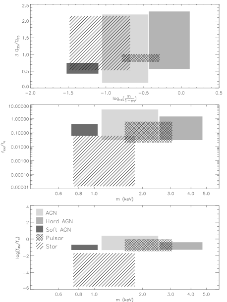
Figure 7: The parameter spaces described by the sources we have classified in the SMC Wing survey as stars, AGN, ‘hard’ AGN, ‘soft’ AGN and pulsars (see Sections 7.5.1–7.5.3). We have included the Bar pulsars (Edge et al., 2004) in the pulsar group. The star category is plotted as a hatched region, the AGN in light grey, the ‘hard’ AGN in mid-grey, the ‘soft’ AGN in dark grey and the pulsars as a cross-hatched region.

7.5.1 Stars

By combining the quantile and X-ray to optical flux ratio data we identify 34 stars in the SMC Wing Survey. Using the SIMBAD database we have found the spectral types for four of these sources and find two F, one G and one M star. In two cases we have classified a source as a star based on optical data alone. One of the objects flagged as a possible HMXB in Section 7.2 (catalogue source 263) is subsequently identified as a star from its position on the combined quantile analysis and flux ratio diagrams.

7.5.2 AGNs

The majority of the sources in our survey are candidate AGNs. Based on the quantile median ($m$) of an object we have classified the source as either an AGN ($1.1<m<2.5$) or a ’hard’ AGN ($m>2.5$). We find 185 of the former and 32 of the latter. In addition, we identify a subset of sources which we have called ’soft’ AGNs which have $m<1.1$ (see Figure 8). This sub-class is based on the classification of one of the original sources as an AGN (see Section 7.5) which falls in a region separated from the location of the stars and AGNs. Optical spectroscopy is needed to determine the nature of these nine sources, and confirm whether or not they are AGNs.

According to the relation from Hornschemeier et al. (2001) the $\log(f_{\rm X_{\rm S}}/f_{R})$ ratio for AGNs should be $0\pm 1$. We find that a small fraction of the sources that we have classified as AGNs have $\log(f_{\rm X_{\rm S}}/f_{R})<-1$. This could indicate that we have the wrong optical match, or that the uncertainty on the $R$ magnitude is large. In most of these cases the classification was based on the location of the source in the QCCD, supported by the flux ratio plots.

Figure 8: The same diagrams as in Figure 5 but with the ’soft’ AGNs and the HMXB candidate included. The symbols represent the same classifications as in Figure 5. Only the sources classified in Sections 7.1–7.4 are shown. The sources classified as ’soft’ AGNs are marked with filled diamonds, and the HMXB candidate is marked with a filled square.

7.5.3 HMXBs

Apart from the four already known pulsars we find only one source (catalogue source 19, CXOU J005635.0-732631, RA = 00:56:34.96, Dec. = -73:26:30.6) that was identified as a HMXB candidate in Section 7.2. We note that this object is fainter than the majority of HMXBs identified to date, with $V=18.0$ and $R=17.2$. The other source that met the magnitude and $f_{\rm X_{\rm H}}/f_{V}$ criteria (see Section 7.2) was subsequently identified as a star (see Section 7.5.1). The combined quantile analysis and flux ratio diagrams for the HMXB candidate indicate that it could be categorised as such (see Figure 8). However, the presence of a fainter object, below the catalogue thresholds, closer to the X-ray position cannot be ruled out. Again, optical spectroscopy, or detection of pulsations, is required to determine its true character.

In Figure 7 we plot the parameter spaces described by the sources we have classified as stars, AGN, ‘hard’ AGN, ‘soft’ AGN and the Bar and Wing pulsars.

7.5.4 LMXBs

We do not find any sources that seem to have the characteristics of a LMXB, but we cannot rule out the presence of quiescent sources below our detection threshold of $3.9\times 10^{33}$ erg s^-1.

7.5.5 Others

In addition to the classes given above, we find 35 sources that have optical matches for which an unambiguous classification is not possible, including one source that has only two counts so no quantile information is available. It is likely that for a number of these objects the wrong optical match has been made leading to a discrepancy in the position of the source on the flux ratio plots compared to the QCCD. We have also not attempted to classify the objects that do not have optical counterparts due to the ill defined boundaries for different types of sources on the QCCD.

8 Discussion

For the 523 sources detected in the SMC Wing survey we have been able to find optical matches for 300 of them, and assign preliminary classifications to 265 objects. Our classification method has the advantage that it does not require optical spectra, however, it still requires optical counterparts to be identified. We also note that to classify the remaining 49% of the survey deeper optical surveys are needed, and in some cases better coverage of the Wing.

The majority of the Wing sources are found to be AGNs. In the whole survey we only identify four pulsars (see McGowan et al., 2007) and one HMXB candidate, which compared to the Bar is a small sample. The relatively few pulsars detected in the Wing is perhaps not surprising given the accepted link between regions of H$\alpha$ and star formation, with the main regions of star formation coinciding with the high density H$\alpha$ region in the Bar (Kennicutt et al., 1995). However, in general, the pulsars we detected in the Wing have harder spectra than those in the Bar. It is also remarkable that the only supergiant system so far detected in the SMC, SMC X-1, lies in the Wing. We note that, despite appearances, the SMC is a very three dimensional object. Studies of the Cepheid population by Laney & Stobie (1986) have revealed that the depth of the SMC is up to 10 times its observed width. The two main structures, the Bar and the Wing, could be separated by 10–20 kpc. Could different populations be represented in the two regions?

In the case of the HMXBs if we based our response on the X-ray results alone we could perhaps draw the conclusion that the sources in the Wing and Bar are in fact different. However, taking into account the optical spectral analysis in which the optical counterparts for the pulsars were found to be typical of other HMXBs in the SMC (Schurch et al., 2007; McBride et al., 2007b), different populations seem less likely. This could imply that there is absorption local to the sources which effects the X-ray spectral results.

There is also the possibility that a greater population of HMXBs does exist in the Wing of the SMC, but we were not fortunate enough to catch more than a handful of them when they were switched on. From our studies of 10 years of RXTE data we find that the probability of a Be X-ray transient being in an active phase is only, on average, $\sim 10$% (Figure 4.62, Galache, 2006). Quiescent X-ray transients have been detected previously in the Milky Way with luminosities $<10^{34}$ erg s^-1 (e.g. Negueruela et al., 2000; Campana et al., 2002). The origin of the quiescent luminosity in Be X-ray transients is still under debate, with a number of processes suggested to account for the detected emission (see e.g. Campana et al., 2002; Kretschmar et al., 2004). The two mechanisms detectable from sources located in the SMC are: accretion onto the magnetospheric boundary, the propeller regime (Illarionov & Sunyaev, 1975; Campana & Stella, 2000), and very low rate accretion onto the surface of the neutron star, i.e. residual/leaking accretion (e.g. Stella et al., 1994). The one HMXB candidate that we have identified has a luminosity (at the distance to the SMC) of $3.2\times 10^{33}$ erg s^-1 so it could be a quiescent source.

The lack of HMXBs in the Wing indicates that we are looking at an older population which is confirmed by optical studies of the star formation history of the SMC (e.g. Harris & Zaritsky, 2004). In theory this should increase our chances of detecting LMXBs. Arguably, LMXBs should be well distributed within the SMC, i.e. they should lie in the Bar and the Wing, however, deep looks of the SMC Bar (Nazé et al., 2003) have been unsuccessful in detecting any.

The number of LMXBs expected in the SMC is proportional to the total stellar mass of the galaxy, resulting in a prediction of only one system with an X-ray luminosity of $\geq 10^{35}$ erg s^-1 (see Shtykovskiy & Gilfanov, 2005). However, Garcia et al. (2001) have shown that quiescent LMXBs can be as faint as $2\times 10^{30}$ erg s^-1. To go as deep as that is beyond the capability of current X-ray telescopes, but in 100 ks it would be possible to reach a limit of $\sim 10^{32}$ erg s^-1, sufficient to detect a sample of fainter sources and study their characteristics. If an observation like this were performed in the Wing it could be compared directly with the deep exposures of the Bar (Nazé et al., 2003; Zezas, 2005) and help quantify the LMXB population in the SMC.

Table 2: The SMC Wing Survey Catalogue (only the first 20 sources are shown). The full catalogue is available as Supplementary Material in the electronic edition of the journal. The table is ordered in ascending RA. The sources are classified as the following: star, AGN, pulsar, ’AGN h’ and ’AGN s’ - hard and soft AGN, respectively (see text for details) and ’HMXB?’ - HMXB candidate. The sources with optical matches that were not able to be classified are marked with ’?’.

No	RA	Dec.	Error	Net	S/N	Flux	$m$	$\log_{10}(m/1-m)$	$3Q_{25}/Q_{75}$	$m_{V}$	$m_{R}$	$B-V$	$f_{\rm X_{\rm H}}/f_{V}$	$\log(f_{\rm X_{\rm S}}/f_{R})$	Class
	(J2000)	(J2000)	($\pm\arcsec$)	Cts		($\times 10^{-14}$ erg cm-2 s-1)	(keV)
1	00:54:35.47	-73:19:40.8	4.17	11	3.7	2.31	1.46	-0.83	1.99	19.2	18.3		0.11	-1.23	AGN
2	00:55:03.67	-73:21:10.5	2.43	9	4.2	1.15	1.85	-0.66	1.05	18.8		0.18	0.04		AGN
3	00:55:16.97	-73:23:49.6	1.17	12	5.8	1.30	1.81	-0.67	0.62	19.4	19.2		0.08	-1.12	AGN
4	00:55:17.38	-73:30:08.5	3.13	6	2.9	0.71	1.05	-1.10	0.64		19.4			-1.30	AGN s
5	00:55:24.34	-73:31:11.0	3.97	6	2.8	0.74	0.76	-1.45	0.70
6	00:55:26.45	-73:34:37.6	11.16	6	2.5	0.97	1.52	-0.80	0.64	20.3		0.79	0.13		AGN
7	00:55:32.50	-73:23:16.7	2.51	2	1.0	0.21	-	-	-	20.8	20.6		0.04	-1.35	?
8	00:55:32.94	-73:31:14.4	2.69	9	4.1	1.36	2.17	-0.54	0.93
9	00:55:33.34	-73:18:20.2	2.01	19	8.1	2.51	1.79	-0.68	1.33	19.8	19.4		0.21	-0.75	AGN
10	00:55:45.25	-73:24:45.3	0.96	6	3.1	0.70	1.26	-0.95	1.22	18.7	18.3		0.02	-1.75	star
11	00:55:51.54	-73:31:10.1	0.88	231	74.2	27.4	1.46	-0.83	1.10	18.4		0.61	0.64		AGN
12	00:56:03.63	-73:23:24.6	0.85	15	7.7	1.55	1.54	-0.79	1.24	20.2	19.4		0.19	-0.96	AGN
13	00:56:05.22	-73:29:45.2	2.27	4	2.1	0.55	3.05	-0.29	1.79
14	00:56:11.60	-73:28:51.7	1.45	3	1.6	0.33	1.52	-0.80	2.29
15	00:56:12.39	-73:26:30.4	1.49	4	2.1	1.08	1.68	-0.73	1.36
16	00:56:16.36	-73:25:19.8	0.86	7	3.7	0.73	1.36	-0.89	1.89	20.4		0.26	0.11		AGN
17	00:56:20.27	-73:24:25.9	0.99	4	2.1	0.42	1.87	-0.65	0.83	19.9	19.9		0.04	-1.33	?
18	00:56:24.09	-73:25:06.2	0.88	7	3.6	0.73	2.22	-0.53	0.69	21.0		0.40	0.19		AGN
19	00:56:34.96	-73:26:30.6	0.96	7	3.6	0.75	3.16	-0.26	0.73	18.0	17.2		0.01	-2.16	HMXB?
20	00:56:38.64	-73:28:56.3	1.75	5	2.6	0.66	0.80	-1.38	0.64

References

- Barlow et al. (2006) Barlow E.J., Knigge C., Bird A.J., Dean A.J., Clark D.J., Hill A.B., Molina M., Sguera V., 2006, MNRAS, 372, 224
- Campana & Stella (2000) Campana S., Stella L., 2000, ApJ, 541, 849
- Campana et al. (2002) Campana S., Stella L., Israel G.L., Moretti A., Parmar A.N., Orlandini M., 2002, ApJ, 580, 389
- Coe et al. (2005) Coe M.J., Edge W.R.T., Galache J.L., McBride V.A., 2005, MNRAS, 356, 502
- Cutri et al. (2003) Cutri R.M., et al., 2003, VizieR On-line Data Catalog, 11/246. CDS, France (online publication only)
- Dickey & Lockman (1990) Dickey J.M., Lockman F.J., 1990, ARAA, 28, 215
- Edge et al. (2004) Edge W.R.T., Coe M.J., Galache J.L., McBride V.A., Corbet R.H.D., Markwardt C.B., Laycock S., 2004, MNRAS, 353, 1286
- Filipovic et al. (1998) Filipovic M.D., 1998, A&AS, 127, 119
- Galache (2006) Galache J.L., 2006, PhD Thesis, Univ. Southampton
- Garcia et al. (2001) Garcia M.R., McClintock J.E., Narayan R., Callanan P., Barret D., Murray S.S., 2001, ApJ, 553, 47
- Gardiner & Noguchi (1996) Gardiner L.T., Noguchi M., 1996, MNRAS, 278, 191
- Garmire et al. (2003) Garmire G.P., Bautz M.W., Ford P.G., Nousek J.A., Ricker G.R., 2003, SPIE, 4851, 28
- Grimm, Gilfanov & Sunyaev (2003) Grimm, H.-J., Gilfanov M.R., Sunyaev R.A., 2003, MNRAS, 339, 793
- Haberl & Pietsch (2004) Haberl F., Pietsch W., 2004, A&A, 414, 667
- Harris & Zaritsky (2004) Harris J., Zaritsky D., 2004, AJ, 127, 1531
- Hong et al. (2004) Hong J., Schlegel E.M., Grindlay J.E., 2004, ApJ, 614, 508
- Hong et al. (2005) Hong J., van den Berg M., Schlegel E.M., Grindlay J.E., Koenig X., Laycock S., Zhao P., 2005, ApJ, 635, 907
- Hornschemeier et al. (2001) Hornschemeier A.E., et al., 2001, ApJ, 554, 742
- Illarionov & Sunyaev (1975) Illarionov A.F., Sunyaev R.A., 1975, A&A, 39, 185
- Kennicutt (1991) Kennicutt R.C., Jr., 1991, in Haynes R.F., Milne D.K., eds., Proc. IAU Symp. 148, The Magellanic Clouds. Reidel, Dordrecht, p. 139
- Kennicutt et al. (1995) Kennicutt R.C., Jr., Bresolin F., Bomans D.J., Bothun G.D., Thompson I.B., 1995, AJ, 109, 594
- Kretschmar et al. (2004) Kretschmar P., Wilms J., Staubert R., Kreykenbohm I., Heindl W.A., 2004, Proc. of the 5th INTEGRAL Workshop on the INTEGRAL Universe (ESA SP-552), 16-20 February 2004, Munich, Germany. Scientific Editors: V. Schonfelder, G. Lichti & C. Winkler, p.329
- Laney & Stobie (1986) Laney C.D., Stobie R.S., 1986, MNRAS, 222, 449
- Maccacaro et al. (1988) Maccacaro T., Gioia I.M., Wolter A., Zamorani G., Stocke J.T., 1988, ApJ, 326, 680
- Massey (2002) Massey P., 2002, ApJS, 141, 81
- McBride et al. (2007a) McBride V.A., et al., 2007a, MNRAS, in press (arXiv:0709.0633)
- McBride et al. (2007b) McBride V.A., Coe M.J., Negueruela I., Schurch M.P.E., McGowan K.E., 2007b, MNRAS, submitted
- McGowan et al. (2007) McGowan K.E., et al., 2007, MNRAS, 376, 759
- Monet et al. (2003) Monet D.G., et al., 2003, AJ, 125, 984
- Morrison & McLean (2001) Morrison J.E., McLean B., 2001, GSC-Catalog Construction Team, II, DDA, 32.0603
- Nazé et al. (2003) Nazé Y., Hartwell J.M., Stevens I.R., Manfroid J., Marchenko S., Corcoran M.F., Moffat A.F.J., Skalkowski G., 2003, ApJ, 586, 983
- Negueruela et al. (2000) Negueruela I., Reig P., Finger M.H., Roche P., 2000, A&A, 356, 1003
- Negueruela & Coe (2002) Negueruela I., Coe M.J., 2002, A&A, 385, 517
- Schurch et al. (2007) Schurch M.P.E., Coe M.J., McGowan K.E., McBride V., Buckley D.A., Galache J.L., Corbet R.H.D., 2007, MNRAS, in press (arXiv:0708.0228)
- Shtykovskiy & Gilfanov (2005) Shtykovskiy P., Gilfanov M., 2005, MNRAS, 362, 879
- Stanimirović et al. (1999) Stanimirović S., Staveley-Smith L., Dickey J.M., Sault R.J., Snowden S.L., 1999, MNRAS, 302, 417
- Stella et al. (1994) Stella L., Campana S., Colpi M., Mereghetti S., Tavani M., 1994, ApJ, 423, 47
- Westerlund (1997) Westerlund B., 1997, The Magellanic Clouds, Cambridge Univ. Press, Cambridge
- Zaritsky et al. (2002) Zaritsky D., Harris J., Thompson I.B., Grebel E.K., Massey P., 2002, AJ, 123, 855
- Zezas (2005) Zezas A., 2005, CXO, Prop. 1938