DESY 07-140
SFB/CPP-07-49

Precision for B–meson matrix elements

Abstract

We demonstrate how HQET and the Step Scaling Method for B–physics, pioneered by the Tor Vergata group, can be combined to reach a further improved precision. The observables considered are the mass of the b-quark and the $\mathrm{B_{s}}$–meson decay constant. The demonstration is carried out in quenched lattice QCD. We start from a small volume, where one can use a standard O($a$)-improved relativistic action for the b-quark, and compute two step scaling functions which relate the observables to the large volume ones. In all steps we extrapolate to the continuum limit, separately in HQET and in QCD for masses below $m_{\mathrm{b}}$. The physical point $m_{\mathrm{b}}$ is then reached by an interpolation of the continuum results in $1/m$. The essential, expected and verified, feature is that the step scaling fuctions have a weak mass-dependence resulting in an easy interpolation to the physical point. With $r_{0}=0.5\,{\rm fm}$ and the experimental $\mathrm{B_{\mathrm{s}}}$ and K masses as input, we find $F_{\rm B_{\rm s}}=191(6)$ MeV and the renormalization group invariant mass $M_{\mathrm{b}}=6.88(10)$ GeV, translating into $\kern 1.0pt\overline{\kern-1.0ptm\kern-1.0pt}\kern 1.0pt_{\mathrm{b}}(\kern 1.0pt\overline{\kern-1.0ptm\kern-1.0pt}\kern 1.0pt_{\mathrm{b}})=4.42(6)$ GeV in the ${\rm\overline{MS\kern-0.50003pt}\kern 0.50003pt}$ scheme. This approach seems very promising for full QCD.

1 Introduction

It has long been realized that B-meson decays and mixing have a significant potential for the search for physics beyond the Standard Model of particle physics. Unfortunately, the comparison of experimental results from BaBar and Belle to the Standard Model has not yet revealed such effects. An even higher precision in both future experiments and the corresponding “predictions” of the theory is required if we want to get hints for new particles or interactions in this way.

The most promising method for the computation of QCD matrix elements with at most one hadron in initial and final states is lattice QCD. Contrary to what is sometimes reported, it is, however, a very non-trivial task to achieve precisions at the (few) percent level, keeping all systematic uncertainties under control. This is particularly so in B-physics, where the difficulty of simulating light quarks with masses that make contact to the regime where chiral perturbation theory is applicable meets the additional requirement of correctly describing the physics of the heavy b-quark. The former requires lattices of a large enough physical size, say $2-3\,{\rm fm}$ across and the latter a small lattice spacing, $a$, or the control of an effective theory (see [?,?,?,?,?] for more detailed accounts of the difficulties and recent progress). In this letter we exclusively discuss a method to cope with the discretization errors associated with the heavy quark dynamics. The light quark is simply taken to be the strange quark and for the purpose of testing the methodology we work in the quenched approximation. The light (dynamical) quark simulations are an entirely separate issue, where fortunately significant progress has recently been made [?,?,?,?,?,?,?,?,?].

The basic idea of the approach investigated here is the fact that b-quarks can be simulated (quite) straightforwardly in a space-time volume with a linear extent of $L_{0}={\rm O}(0.5\,{\rm fm})$ [?,?]. In such a volume the lattice spacing can be chosen small enough such that observables can be computed with a relativistic action for the heavy quark. The continuum limit is reachable by a short, controlled, extrapolation. Starting from this simple idea, two different roads have been taken in the past [?,?,?] and a third one has recently been explored [?].

In the first the (continuum) observables in the small volume serve to determine the parameters of HQET non-perturbatively and then the physical (large volume) matrix elements are computed in this effective theory. By including $1/m_{{\rm b}}$-corrections a good overall precision is attainable [?].

In the second way, one remains in the relativistic theory, and computes the finite size effects of the observables iteratively ($L_{0}\to L_{1}=sL_{0}\to L_{2}=s^{2}L_{0}\ldots$). As one increases the volume also the lattice spacing is increased and one has to reduce the mass, $m_{\mathrm{h}}$, of the actually simulated quark to remain with $am_{\mathrm{h}}\ll 1$. The physical mass of the b-quark is then reached by an extrapolation.

Here we demonstrate how the two approaches can be combined by constraining the extrapolation to the physical quark mass with calculations in the effective theory; extrapolations are turned into interpolations and an even higher precision as well as confidence is reached.

2 Strategy

We are interested in computing an observable $O$, which, in addition to the light quark masses, depends on the mass, $m_{\rm h}$, of a heavy quark. Its exact definition will be mentioned when it becomes relevant. In a Monte Carlo computation the observable depends in addition on the linear extent $L$ of the simulated space-time volume. This finite size effect is negligible when $L$ is large enough, which we here assume to be the case for $L\geq L_{N}$. Following [?,?], we express $O$ as a product of factors,

$$O(m_{\rm h},L_{\infty})=O(m_{\rm h},L_{0})\,{O(m_{\rm h},L_{1})\over O(m_{\rm h},L_{0})}\,\cdots\,{O(m_{\rm h},L_{N})\over O(m_{\rm h},L_{N-1})}\,.$$ (2.1)

Here $L_{0}$ is chosen small enough such that with an affordable effort lattices with a spacing $a\ll 1/m_{\rm h}$ can be used and the continuum limit can be reached by an extrapolation of $O$ computed with a relativistic ${\rm O}(a)$-improved action. For the b-quark this means that $a\approx 0.012$ fm can be used. In a small volume the details of the topology, boundary conditions and the exact choice of observables are relevant. We here note only that choosing Schrödinger functional boundary conditions makes such numerical computations affordable also when dynamical quarks are included [?]. We come back to these details in Sect. 3.

The remaining factors in eq. (2.1) describe the dependence on $L$. They are called step scaling functions. In their original version [?], they depended only on $L_{i}$ (or equivalently a renormalized coupling $\bar{g}(L_{i})$), but here we have an additional dependence on the mass of the heavy quark. It is convenient to replace the latter by the dimensionless observable

$$x\equiv{1\over L\,m_{\rm PS}(m_{\rm h},L)}={1\over Lm_{\rm h}}+{\rm O}\left(\hbox{$1\over\left(L\,m_{\rm h}\right)^{2}$}\right)\,,$$ (2.2)

constructed from a finite volume pseudoscalar heavy-light mass, $m_{\rm PS}$. It will then also be used as the HQET expansion parameter instead of the inverse of the heavy quark mass. The indicated HQET expansion assumes that $L$ is kept fixed; see e.g. [?,?] for more details; it will be used later. First we define the generic step scaling function

$$\sigma_{O}(x,L)\equiv{O(m_{\rm h},L)\over O(m_{\rm h},L/s)}\,,\quad$$ (2.3)

(with $x$ from eq. (2.2)) where the scale factor $s$ as well as any other quark masses are kept fixed and are not indicated explicitly.

In particular, the step scaling function of the pseudoscalar mass itself,

$$\sigma_{\rm m}(x,L)\equiv{m_{\rm PS}(m_{\rm h},L)\over m_{\rm PS}(m_{\rm h},L/s)}\,,\quad$$ (2.4)

is of central importance. Starting from the experimentally determined mass, $m_{\mathrm{B_{\mathrm{s}}}}=5.3675(18)\,{\rm GeV}$ and $L_{N}$ large enough, it serves to locate the physical points $x_{i}$ via

$$x_{N}=1/(L_{N}m_{\mathrm{B_{\mathrm{s}}}})\,,\quad x_{i-1}=s\,\sigma_{\rm m}(x_{i},L_{i})\,x_{i}\,.$$ (2.5)

The numerical results of all step scaling functions have to be evaluated at these points. eq. (2.1) is then rewritten as

$$O(m_{\rm h},L_{\infty})=O(m_{\rm h},L_{0})\,\sigma_{O}(x_{1},L_{1})\,\cdots\,\sigma_{O}(x_{N},L_{N})\,.$$ (2.6)

Increasing $i$ in eq. (2.5) successively, the computation of the step scaling functions in the relativistic theory at the physical mass requires lattice resolutions $L_{i}/a$ which become larger by a factor $s$ in each step. This is not affordable in practice. Thus the idea of [?,?] was to compute $\sigma_{O}(x,L_{i})$ for a range of $x$ (and thus quark masses) such that $x\geq s^{i}x_{i}\approx x_{0}$ and to extrapolate $x\to x_{i}$. In other words in each step (starting from $L_{0}$) the maximal quark mass which is simulated is reduced by about a factor $s$. As expected from the fact that everywhere one is in the situation $x\ll 1$, the slopes in these extrapolations turned out to be rather small and the extrapolations could thus be carried out. For an illustration of the $x$-dependence as it comes out in practice, one may look ahead at our final results, Fig. 3.

Our main point in this paper is that these extrapolations can be turned into interpolations by computing the limiting behavior for small $x$ directly in HQET,

$$\sigma_{O}(x,L)=\sigma_{O}^{(0)}(L)+{\rm O}(x)\,.$$ (2.7)

As usual in QCD, this large mass expansion is accompanied by logarithms due to anomalous dimensions in the effective theory; ${\rm O}(x)$ thus stands for at least one power of $x$ accompanied by powers of $\log(x)$. For $\sigma_{\rm m}$, the lowest order term is predicted by the theory to be one, while for the first order in $x$, a computation in the static approximation of HQET (${\mathcal{L}}_{\rm{stat}}=\overline{\psi}_{\rm h}D_{0}\psi_{\rm h}$) is required,

$$\sigma_{\rm m}(x,L)=1+\sigma_{\rm m}^{\rm stat}(L)\,x+{\rm O}(x^{2})\,.$$ (2.8)

The static term, which comes from the ${\rm O}(1/(Lm_{\rm h})^{2})$ term in eq. (2.2), is not accompanied by logarithms, see Sect. 3.2. For the case of the decay constant already the lowest order term is given by a non-perturbative computation in the static approximation,

$$\sigma_{\rm f}^{(0)}(L)=\sigma_{\rm f}^{\rm stat}(L)\,.$$ (2.9)

As a further application of this method we compute the mass of the b-quark starting from the physical meson mass $m_{\mathrm{B_{\mathrm{s}}}}$. To this end we define the ratio

$$\rho(x,L)\equiv{m_{\rm PS}(m_{\rm h},L)\over M_{\rm h}}$$ (2.10)

of the meson mass to the renormalization group invariant (RGI) quark mass, $M_{\rm h}$ (see e.g. [?] for its definition). It provides the connection

$$M_{\rm b}={m_{\mathrm{B_{\mathrm{s}}}}\over\rho(x_{0},L_{0})\,\sigma_{\rm m}(x_{1},L_{1})\,\ldots\,\sigma_{\rm m}(x_{N},L_{N})}\,.$$ (2.11)

between the physics input $m_{\mathrm{B_{\mathrm{s}}}}$ and the RGI b-quark mass.

Note that the only approximation made in the above equations is to neglect finite size effects in the volume of linear extent $L_{N}$.

3 Finite volume observables

3.1 Relativistic QCD

Suitable finite volume observables are defined in the QCD Schrödinger functional  [?,?] with a space-time topology $L^{3}\times T$, where $T=2L$ and $C=C^{\prime}=0$ is chosen for the boundary gauge fields, and $\theta=0$ for the phase in the spatial quark boundary conditions.

The O(a)-improved [?,?,?,?,?] heavy-light correlation functions $f_{\rm A}(t),f_{\rm P}(t)$ and $f_{1}$ are defined and renormalized as in [?]. They are illustrated in Fig. 1.

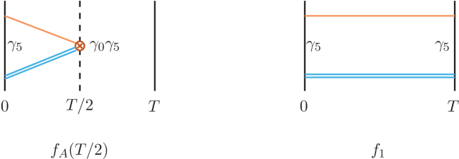
Figure 1: The boundary to axial-current correlator $f_{\rm A}$ and the boundary to boundary correlator $f_{1}$. Dirichlet boundary conditions are imposed at $x_{0}=0$ and $x_{0}=T$.

They allow to define a finite volume pseudoscalar meson decay constant and mass via [?,?]

$$F_{\mathrm{PS}}(m_{\rm h},L) = {-2\over\sqrt{L^{3}m_{\rm PS}(m_{\rm h},L)}}{f_{\rm A}(T/2)\over\sqrt{f_{1}}}\,,$$ (3.12)

$$m_{\rm PS}(m_{\rm h},L) = {1\over 2a}[\ln(f_{\rm A}(T/2-a))-\ln(f_{\rm A}(T/2+a))]\,.$$ (3.13)

We remind the reader that we have a fixed ratio $T/L=2$. Therefore the time separation in the correlation functions grows when $L$ grows. Indeed, as discussed in detail in [?], these quantities approach the physical ones in the large $L$ limit,

$$\lim_{L\to\infty}m_{\rm PS}(m_{\rm b},L)=m_{\mathrm{B_{\mathrm{s}}}}\,,\qquad\lim_{L\to\infty}F_{\mathrm{PS}}(m_{\rm b},L)=F_{\rm B_{\rm s}}\,.$$ (3.14)

with corrections which (asymptotically) are exponentially small in $L$. The associated step scaling functions are defined as

$$\sigma_{\rm f}(x,L)={F_{\mathrm{PS}}(m_{\rm h},L)\sqrt{m_{\rm PS}(m_{\rm h},L)}\over F_{\mathrm{PS}}(m_{\rm h},L/s)\sqrt{m_{\rm PS}(m_{\rm h},L/s)}}\,,\qquad x={1\over L\,m_{\rm PS}(m_{\rm h},L)}\,,$$ (3.15)

and $\sigma_{\mathrm{m}}$ as in eq. (2.4).

3.2 HQET

In the static approximation of HQET, unrenormalized correlation functions $f_{\rm A}^{\rm stat}$ and $f_{1}^{\rm stat}$ are defined in complete analogy to the relativistic ones [?] (see [?] for an introduction). As in these references, we use the RGI static axial current, related to the bare one by a factor $Z_{\rm A,RGI}^{\rm stat}$. It serves to define the RGI ratio ,

$$Y_{\rm RGI}(L)=Z_{\rm A,RGI}^{\rm stat}{f_{\rm A}^{\rm stat}(T/2)\over\sqrt{f_{1}^{\rm stat}(L)}}\,,$$ (3.16)

which is related to the QCD decay constant $F_{\mathrm{PS}}$ via

$$F_{\mathrm{PS}}(m_{\rm h},L)\sqrt{L^{3}m_{\rm PS}(m_{\rm h},L)}=-2C_{\rm PS}(M_{\rm h}/\Lambda_{\rm\overline{MS\kern-0.35002pt}\kern 0.35002pt})\times Y_{\rm RGI}(L)+{\rm O}(x)\,.$$ (3.17)

The function $C_{\rm PS}(M_{\rm h}/\Lambda_{\rm\overline{MS\kern-0.35002pt}\kern 0.35002pt})$, discussed in [?,?], originates from the matching of QCD and the effective theory. In its numerical evaluation we use the anomalous dimension, $\gamma^{\rm PS}$ in the notation of [?]. With the 3-loop term extracted from [?] its uncertainty is estimated to be negligible [?] compared to our other errors. Just like $Z_{\rm A,RGI}^{\rm stat}$, it is needed only for $F_{\mathrm{PS}}(m_{\rm h},L_{0})$; it cancels out in the step scaling functions.

The pseudoscalar finite volume mass has an HQET expansion [?]

$$m_{\rm PS}(m_{\rm h},L)=m_{\rm h}+\delta m+\Gamma_{\rm stat}(L)+{\rm O}(1/m_{\rm h})\,,$$ (3.18)

with

$$\Gamma_{\rm stat}(L)={1\over 2a}[\ln(f_{\rm A}^{\rm stat}(T/2-a))-\ln(f_{\rm A}^{\rm stat}(T/2+a))]\,,$$ (3.19)

where again we do not need to specify the renormalization scheme for $m_{\rm h}$, but it is important that the counterterm $\delta m$ cancels the linear divergence in $\Gamma_{\rm stat}$ and the combination $\delta m+\Gamma_{\rm stat}(L)$ is of order $\Lambda_{\mathrm{QCD}}$. Inserting eqs. (3.17,3.18) into eqs. (3.15,2.4), we arrive at eqs. (2.9,2.8) with the static step scaling functions

$$\sigma_{\rm f}^{\rm stat}(L) = {1\over s^{3/2}}{Y_{\rm RGI}(L)\over Y_{\rm RGI}(L/s)}\,,$$ (3.20)

$$\sigma_{\rm m}^{\rm stat}(L) = L\,[\Gamma_{\rm stat}(L)-\Gamma_{\rm stat}(L/s)]\,.$$ (3.21)

Here the renormalizations $Z_{\rm A,RGI}^{\rm stat}\times C_{\rm PS}$ and $\delta m$ cancel, which shows that these static step scaling functions are not accompanied by any logarithmic terms (in $m_{\mathrm{h}}$ or $x$).

In our numerical investigation we will compute them precisely by using the static action denoted by HYP2 in [?] (see also [?]), and the corresponding ${\rm O}(a)$-improvement coefficients for the static axial current.

4 Results in the quenched approximation

We employ the non-perturbatively O(a)-improved Wilson action [?,?]. The data at finite heavy quark mass are taken from [?,?]. As there, we choose $N=2$ steps, $s=2$ and $L_{0}=0.4\,{\rm fm}$. The length scale is set by $r_{0}=0.5\,{\rm fm}$ [?] using the parametrizations of $r_{0}/a$ as a function of the bare coupling $g_{0}$ from [?,?]. The light quark mass is set to the strange quark mass by fixing the RGI-mass to $M_{{\rm s}}=0.1346(55)\,{\rm GeV}$ as previously determined from the Kaon mass in the quenched approximation [?]. The RGI-mass is related to the bare one by a non-perturbatively computed renormalization factor $Z_{\rm m}$ [?], see e.g. [?] for details.

$L[{\rm fm}]$	$x$	$\sigma_{\mathrm{m}}(x,L)$	$\sigma_{\mathrm{f}}(x,L)$
1.6	0.0581	1.069(5)	0.929(32)
	0.0670	1.081(6)	0.912(27)
	0.0720	1.087(7)	0.900(24)
0.8	0.0804	1.012(6)	0.4198(45)
	0.0884	1.014(6)	0.4193(45)
	0.1204	1.018(8)	0.4169(43)
		$\rho(x,L)$	$\varphi(x,L)$
0.4	0.0933	0.744(09)	3.120(45)
	0.0990	0.754(09)	3.097(45)
	0.1472	0.837(12)	2.911(43)
	0.2768	-	2.534(40)
	0.2885	-	2.505(40)

Table 1: Finite mass observables after continuum extrapolation. Physical units are set through $r_{0}=0.5\,{\rm fm}$. Statistical errors of $x$ due to $m_{\rm PS}$ have been changed to errors in the $x$-dependent observables.

4.1 At finite heavy quark mass

The data of [?,?] have been reanalyzed. The step scaling functions were first defined at a fixed value of $r_{0}M_{\mathrm{h}}$ as in those references. Their continuum limit was taken by an extrapolation linear in $(a/L)^{2}$, making use of different definitions of $M_{\mathrm{h}}$ at finite lattice spacing and of the fact that the continuum limit is independent of such details. Correlations between observables computed on the same gauge configurations were taken into account. The statistical uncertainties of the regularization dependent part of the renormalization constants and the lattice spacing were included before performing the continuum limit extrapolations, the uncertainty of the regularization independent part of the renormalization constants is added in the continuum limit; all these do not appear as a separate uncertainties, rather they are included in the quoted errors. For their detailed accumulation we refer to [?]. An impression on the quality of the continuum extrapolations is easily obtained from the graphs in [?,?,?]. Since here our emphasis is on the use of the static approximation, we do not reproduce those details. The continuum values of the step scaling functions were then interpolated in the pseudoscalar mass to a few selected values of $x$. These are listed in Table 1 together with $\rho$, eq. (2.10) and

$$\varphi(x,L)=L^{3/2}F_{\rm PS}\sqrt{m_{\rm PS}}\,.$$ (4.22)

$L_{1}/a$	$\beta$	$a\Gamma^{\rm stat}(L_{1})$	$a\Gamma^{\rm stat}(L_{2})$	$\sigma_{\mathrm{m}}^{\rm stat}(L_{2})$
8	5.9598	0.3183(8)
8.92	6.0219	0.3000(5)	0.4053(49)	1.878(88)
10	6.0914	0.2805(6)
12	6.2110	0.2533(6)
13.41	6.2885	0.2360(5)	0.3011(33)	1.745(89)
16	6.4200	0.2114(7)
16.64	6.4500	0.2067(6)	0.2564(09)	1.654(35)
17.64	6.4956	0.1997(6)	0.2461(14)	1.637(54)
24	6.7370	0.1722(16)
continuum				1.561(53)

Table 2: Numerical results in static approximation for $L_{1}=0.8\,{\rm fm}\,,\;L_{2}=2L_{1}$. The rows with non-integer $L_{1}/a$ list interpolated values for $a\Gamma^{\rm stat}(L_{1})$, while $a\Gamma^{\rm stat}(L_{2})$ are the large volume numbers of [?,?,?].

${L_{0}/a}$	$\beta$	$a\Gamma^{\rm stat}(L_{0})$	$a\Gamma^{\rm stat}(L_{1})$	$\sigma_{\mathrm{m}}^{\mathrm{stat}}(L_{1})$	$Y(L_{0})$	$Y(L_{1})$	$\sigma_{\mathrm{f}}^{\mathrm{stat}}(L_{1})$
6	6.2110	0.2272(9)	0.2558(18)	0.343(24)	-1.805(03)	-2.221(13)	0.4350(27)
8	6.4200	0.1958(9)	0.2154(11)	0.315(23)	-1.837(05)	-2.266(13)	0.4361(26)
12	6.7370	0.1561(8)	0.1663(17)	0.245(46)	-1.881(06)	-2.279(28)	0.4284(55)
16	6.9630	0.1355(7)	0.1426(14)	0.230(50)	-1.899(07)	-2.344(35)	0.4366(67)
24	7.3000				-1.918(10)
continuum				0.233(36)			0.4337(44)

Table 3: Numerical results in static approximation for $L_{0}=0.4\,{\rm fm}$ and $L_{1}=2L_{0}$.

${L_{0}\over a}$	$\beta$	$Z_{\rm A}^{\rm stat}({L_{0}\over a},g_{0})$	${L_{1}\over a}$	$\beta$	$Z_{\rm A}^{\rm stat}({L_{1}\over a},g_{0})$
8	6.4200	0.8745(21)	12	6.2110	0.7904(38)
12	6.7370	0.8534(10)	16	6.4200	0.7672(45)
16	6.9630	0.8408(21)	24	6.7370	0.7651(53)
24	7.3000	0.8308(21)	32	6.9630	0.7556(48)

Table 4: Renormalization factors for the static axial current at renormalization scales $\mu=1/L_{0}$ and $\mu=1/L_{1}$ with $L_{0}=0.4\,{\rm fm}$ and $L_{1}=0.8\,{\rm fm}$.

4.2 In static approximation

We turn to the main new element in our numerical computations. We start with the static step scaling function $\sigma_{\mathrm{m}}^{\mathrm{stat}}(L_{2})$, requiring the computation of $\Gamma_{\rm stat}(L_{1})$ and $\Gamma_{\rm stat}(L_{2})$, for several fixed values of $g_{0}$ followed by a continuum extrapolation. However, it is a central element of our strategy that $L_{2}\approx 1.6\,{\rm fm}$ is large enough such that finite volume effects are negligible. Thus we can replace $\Gamma_{\rm stat}(L_{2})$ by $E_{\rm stat}$, the “mass” of a static-strange bound state in large volume which is known from [?,?,?] in the range $6.0219\leq\beta=6/g_{0}^{2}\leq 6.4956$. We have computed $\Gamma_{\mathrm{stat}}(L_{1})$ for $L/a=8,10,12,16,24$, spanning a wider range in $\beta$ and allowing easily for an interpolation to the values of $\beta$ where $E_{\rm stat}$ is known. All of this was done for the HYP2 static action [?] and for the tree-level as well as the one-loop improved static-light axial current. Differences between the two turned out to be far below our statistical precision of order $1-3\,{\rm MeV}$. The continuum extrapolation of $\sigma_{\mathrm{m}}^{\mathrm{stat}}(L_{2})$, listed in Table 2, is well controlled, see Fig. 2.

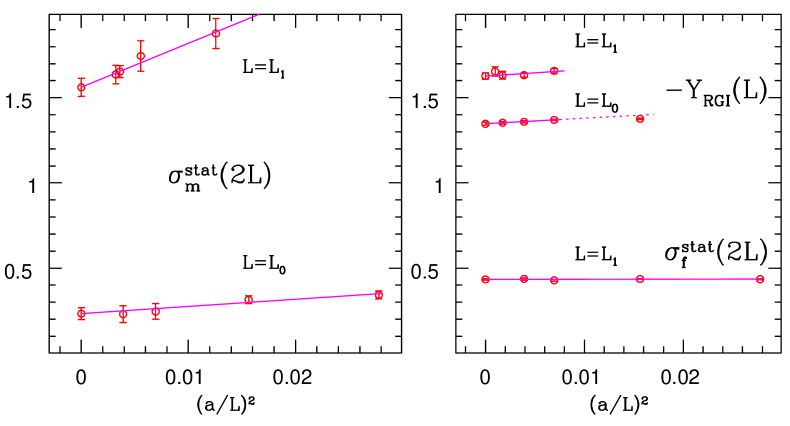
Figure 2: Continuum extrapolations of static results. The extrapolated values with their errors are shown at $a/L=0$.

Similarly we profit from previous work in large volume in the computation of $\sigma_{\mathrm{f}}^{\mathrm{stat}}(L_{2})$, eq. (3.20). In that case the continuum value

$$Y_{\rm RGI}(L_{2})=-4.65(19)\,,$$ (4.23)

is known from [?,?]. It remains to compute

$$Y_{\rm RGI}(L_{1}) = {\Phi_{\rm RGI}\over\Phi_{\rm SF}(\mu)}\times Z_{\rm A}^{\rm stat}(L^{\prime}/a,g_{0})\times Y(L_{1}/a,g_{0})\,,\quad L^{\prime}=1/\mu\,.$$ (4.24)

Here

$$Y(L/a,g_{0})={f_{\rm A}^{\rm stat}(L)\over\sqrt{f_{1}^{\rm stat}(L)}}\,$$ (4.25)

is the unrenormalized version of eq. (3.16) and $Z_{\rm A}^{\rm stat}(L^{\prime}/a,g_{0})$ is the factor, introduced in [?], to renormalize the static axial current in the (“new”) SF scheme, non-perturbatively at renormalization scale $\mu=1/L^{\prime}$. Finally ${\Phi_{\rm RGI}\over\Phi_{\rm SF}(\mu)}$ relates any matrix element of the axial current in the SF scheme to the RGI matrix element. At the renormalization point $L^{\prime}=L_{1}$ its non-perturbative value

$${\Phi_{\rm RGI}\over\Phi_{\rm SF}(1/L_{1})}=0.928(2)\,$$ (4.26)

is easily extracted from the results in [?]. We have computed the missing factors $Z_{\rm A}^{\rm stat}(L^{\prime}/a,g_{0})\,,Y(L_{1}/a,g_{0})$ for various values of $L_{1}/a$, setting $L^{\prime}=L_{1}$, see Table 4. Note that following the exact definition of [?], $\theta=1/2\,,T=L^{\prime}$ is employed for $Z_{\rm A}^{\rm stat}$ and the computation is carried out at zero (light) quark mass – in contrast to the evaluation of $Y$ (and all other quantities).

The continuum limit (Fig. 2)

$$Y_{\rm RGI}(L_{1})=-1.628(19)$$ (4.27)

is combined with (4.23) to get

$$\sigma_{\rm f}^{\rm stat}(L_{2})=1.010(43).$$ (4.28)

In the computation of the static step scaling functions $\sigma^{\mathrm{stat}}(L_{1})$ (Table 3, Fig. 2) we followed straightforwardly their definitions. Finally,

$${\Phi_{\rm RGI}\over\Phi_{\rm SF}(1/L_{0})}=0.846(6)\,.$$ (4.29)

from [?] together with $Y(L_{0}/a,g_{0})\,,Z_{\rm A}^{\rm stat}(L_{0}/a,g_{0})$, Tables 3 and 4, yields

$$Y_{\rm RGI}(L_{0})=-1.347(13)\,$$ (4.30)

by a continuum extrapolation again illustrated in Fig. 2.

4.3 Interpolation to the physical point

We now combine the static results with the relativistic ones, through linear and quadratic interpolations in $x$. Namely we fit for the parameters $m_{j}(L_{i})$ and $e_{j}(L_{i})$ in

$$\sigma_{m}(x,L_{i}) = 1+m_{1}(L_{i})\,x+m_{2}(L_{i})\,x^{2}\,,$$ (4.31)

$$\sigma_{\rm m}^{\rm stat}(L_{i}) = m_{1}(L_{i})\,,$$ (4.32)

$$\sigma_{\rm f}(x,L_{i}) = e_{0}(L)+e_{1}(L_{i})\,x+e_{2}(L_{i})\,x^{2}\,,$$ (4.33)

and then insert the fit functions eq. (4.31) and eq. (4.33) into eq. (2.11) and eq. (4.34). Note that the first two equations are fit together. The static $\sigma_{\rm m}^{\rm stat}(L_{i})$ enter eq. (4.32) as data points and $\sigma_{\rm f}^{\rm stat}(L_{i})$ are data at $x=0$ in eq. (4.33). As seen in Fig. 2, the quadratic terms are moderate in the whole range and in particular at the physical points $x_{i}$ the differences between the static results and the interpolated ones are rather small. As an illustration of the effect of the static results we also carry out an analysis where they are not taken into account. The numbers in Table 5 show that the statistical errors in the step scaling functions are significantly reduced by including the static constraints. Furthermore we can perform the consistency check of including quadratic terms only when the static constraints are used. The agreement between linear and quadratic interpolations is very reassuring.

$i$	$\sigma_{\mathrm{m}}(x_{i},L_{i})$			$\sigma_{\mathrm{f}}(x_{i},L_{i})$		Fit
2	1.0330(11)	1.0258(21)		0.985(31)		quadratic
2	1.0319(11)	1.0276(22)		0.977(29)	1.002(54)	linear
1	1.0092(18)	1.0074(33)		0.4243(36)		quadratic
1	1.0093(15)	1.0072(32)		0.4260(31)	0.4223(48)	linear

Table 5: Step scaling functions inter/extra-polated to the physical points $x_{2}=0.022974(8)$, $x_{1}=0.04746(5)$ and $x_{1}^{\rm QCD}=0.04741(10)$, where the latter originates from the fits to only the finite heavy quark mass data. The left–side column of each $\sigma$ is the number including the static constraint, the right–side one is without.

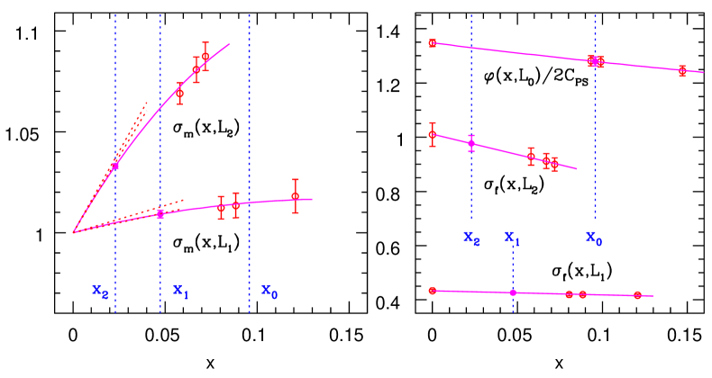
Figure 3: Interpolations to the physical points are shown by the filled circles. For $\sigma_{\mathrm{m}}$, the static constraints are illustrated as the error band of the static result $1+\sigma_{\mathrm{m}}^{\mathrm{stat}}x$. On the right hand side, the static results enter as data points at $x=0$.

For $\rho(x,L_{0})$ and $F_{\mathrm{PS}}(x,L_{0})$ the relativistic simulations straddle the physical point $x=x_{0}$ and, for the decay constant, the static data do not sensitively improve the precision on the interpolated point. However, as an illustration how HQET does describe these quantities, we also show eq. (4.30) together with the data at finite $x$ in Fig. 3; in that case the interpolation yields $L_{0}^{3/2}F_{\mathrm{PS}}\sqrt{m_{\rm PS}}/(2C_{\rm PS})=1.279(17)$ or $\varphi(x_{0},L_{0})=3.107(41)$ and $\rho(x_{0},L_{0})=0.7485(9)$.

Our final large volume results from eq. (2.11) and

$$F_{\rm B_{\rm s}}=\varphi(x_{0},L_{0})\,\sigma_{\rm f}(x_{1},L_{1})\,\sigma_{\rm f}(x_{2},L_{2})\,L_{0}^{-3/2}\,m_{\mathrm{B_{\mathrm{s}}}}^{-1/2}$$ (4.34)

are

$$F_{\rm B_{\rm s}}=191(6)\,{\rm MeV}\,,\quad M_{\rm b}=6.88(10)\,{\rm GeV}\Longrightarrow\kern 1.0pt\overline{\kern-1.0ptm\kern-1.0pt}\kern 1.0pt_{\mathrm{b}}(\kern 1.0pt\overline{\kern-1.0ptm\kern-1.0pt}\kern 1.0pt_{\mathrm{b}})=4.42(6)\,{\rm GeV}\,.$$ (4.35)

Here the conversion to the running mass in the ${\rm\overline{MS\kern-0.50003pt}\kern 0.50003pt}$-scheme is done with the 4-loop RG equations (for $N_{\rm f}=0$ and $\Lambda_{\rm\overline{MS\kern-0.35002pt}\kern 0.35002pt}^{(0)}=238(19)\,{\rm MeV}$ [?]).

5 Conclusions and outlook

We have followed a general strategy for computing B-meson observables. Starting from a finite volume, where the observables are straightforwardly computable in relativistic lattice QCD, we evaluated step scaling functions which describe the finite size effects. The latter are not directly computable at the physical points since for accessible lattices $am_{{\rm b}}\geq 1$. Previously these functions have either been computed by an extrapolation in the heavy quark mass to the physical $m_{{\rm b}}$ [?,?] or they have been computed in HQET [?,?]. Here we have demonstrated how the two approaches can be combined to further increase precision and confidence in the results.

Figure 3, which is a continuum graph, shows that the static (lowest order HQET) results match very well onto the finite mass step scaling functions. We therefore have excellent control over the heavy quark mass dependence – if desired from below the charm quark mass to the b-quark mass and beyond.

Our final numbers for decay constant and b-quark mass, eq. (4.35), agree well with the previous estimates of [?,?,?,?,?] where the same experimental data was used as input.

In our results, Fig. 3, one notices that the corrections to the static approximation are very small at the b-quark mass. This represents an intriguing demonstration of the precision and usefulness of HQET for B-physics. Although our exercise was in the quenched approximation, such a qualitative result may well be carried over to (full) QCD.

Concerning the application of the strategy to QCD, the attentive reader will have noticed that in our computations we extensively relied on the knowledge of a reference scale ($r_{0}/a$) over a large range of lattice spacings $a$. This luxury is not available in full QCD – and will not be for a while to come. However, with the knowledge of the running coupling of [?], one can properly set the scale also for small lattice spacings. We further note that the finite volume computations which are needed in this strategy require a significantly smaller effort than the large volume ones.

We therefore conclude that the here investigated method is very promising for the near future where we expect that high precision can be reached for B-physics. Note that the strategy may be extended to other observables such as mass splittings [?,?] and form factors [?].

Acknowledgement

It is a pleasure to thank Michele Della Morte and Giulia Maria de Divitiis for useful discussions as well as some practical help. We thank NIC for allocating computer time on the APEmille computers at DESY Zeuthen to this project and the APE group for its help. This project has been supported by the DFG in the SFB Transregio 9 “Computational Particle Physics” and by the European community through EU Contract No. MRTN-CT-2006-035482, “FLAVIAnet”.

References

- [1] A.S. Kronfeld, Nucl. Phys. Proc. Suppl. 129 (2004) 46, hep-lat/0310063.
- [2] R. Sommer, ECONF C030626 (2003) FRAT06, hep-ph/0309320.
- [3] S. Hashimoto and T. Onogi, Ann. Rev. Nucl. Part. Sci. 54 (2004) 451, hep-ph/0407221.
- [4] T. Onogi, PoS LAT2006 (2006) 017, hep-lat/0610115.
- [5] R. Sommer, (2006), hep-lat/0611020.
- [6] M. Hasenbusch, Phys. Lett. B519 (2001) 177, hep-lat/0107019.
- [7] M. Lüscher, Comput. Phys. Commun. 165 (2005) 199, hep-lat/0409106.
- [8] L. Del Debbio, L. Giusti, M. Lüscher, R. Petronzio and N. Tantalo, JHEP 02 (2006) 011, hep-lat/0512021.
- [9] C. Urbach, K. Jansen, A. Shindler and U. Wenger, Comput. Phys. Commun. 174 (2006) 87, hep-lat/0506011.
- [10] M.A. Clark and A.D. Kennedy, (2006), hep-lat/0608015.
- [11] H.B. Meyer et al., Comput. Phys. Commun. 176 (2007) 91, hep-lat/0606004.
- [12] M. Lüscher, (2007), arXiv:0706.2298 [hep-lat].
- [13] M.A. Clark, PoS LAT2006 (2006) 004, hep-lat/0610048.
- [14] RBC and UKQCD, C. Allton et al., Phys. Rev. D76 (2007) 014504, hep-lat/0701013.
- [15] ALPHA, J. Heitger and R. Sommer, Nucl. Phys. Proc. Suppl. 106 (2002) 358, hep-lat/0110016.
- [16] R. Sommer, (2002), hep-lat/0209162.
- [17] ALPHA, J. Heitger and R. Sommer, JHEP 02 (2004) 022, hep-lat/0310035.
- [18] M. Guagnelli, F. Palombi, R. Petronzio and N. Tantalo, Phys. Lett. B546 (2002) 237, hep-lat/0206023.
- [19] M. Della Morte, N. Garron, M. Papinutto and R. Sommer, JHEP 01 (2007) 007, hep-ph/0609294.
- [20] H.W. Lin and N. Christ, (2006), hep-lat/0608005.
- [21] G.M. de Divitiis, M. Guagnelli, R. Petronzio, N. Tantalo and F. Palombi, Nucl. Phys. B675 (2003) 309, hep-lat/0305018.
- [22] G.M. de Divitiis, M. Guagnelli, F. Palombi, R. Petronzio and N. Tantalo, Nucl. Phys. B672 (2003) 372, hep-lat/0307005.
- [23] ALPHA, M. Della Morte et al., Comput. Phys. Commun. 156 (2003) 62, hep-lat/0307008.
- [24] M. Lüscher, P. Weisz and U. Wolff, Nucl. Phys. B359 (1991) 221.
- [25] ALPHA, S. Capitani, M. Lüscher, R. Sommer and H. Wittig, Nucl. Phys. B544 (1999) 669, hep-lat/9810063.
- [26] M. Lüscher, R. Narayanan, P. Weisz and U. Wolff, Nucl. Phys. B384 (1992) 168, hep-lat/9207009.
- [27] S. Sint, Nucl. Phys. B421 (1994) 135, hep-lat/9312079.
- [28] B. Sheikholeslami and R. Wohlert, Nucl. Phys. B259 (1985) 572.
- [29] M. Lüscher, S. Sint, R. Sommer and P. Weisz, Nucl. Phys. B478 (1996) 365, hep-lat/9605038.
- [30] M. Lüscher and P. Weisz, Nucl. Phys. B479 (1996) 429, hep-lat/9606016.
- [31] M. Lüscher, S. Sint, R. Sommer, P. Weisz and U. Wolff, Nucl. Phys. B491 (1997) 323, hep-lat/9609035.
- [32] ALPHA, M. Guagnelli et al., Nucl. Phys. B595 (2001) 44, hep-lat/0009021.
- [33] ALPHA, M. Guagnelli, J. Heitger, R. Sommer and H. Wittig, Nucl. Phys. B560 (1999) 465, hep-lat/9903040.
- [34] ALPHA, J. Heitger, Nucl. Phys. B557 (1999) 309, hep-lat/9903016.
- [35] ALPHA, J. Heitger, M. Kurth and R. Sommer, Nucl. Phys. B669 (2003) 173, hep-lat/0302019.
- [36] ALPHA, J. Heitger, A. Jüttner, R. Sommer and J. Wennekers, JHEP 11 (2004) 048, hep-ph/0407227.
- [37] K.G. Chetyrkin and A.G. Grozin, Nucl. Phys. B666 (2003) 289, hep-ph/0303113.
- [38] M. Della Morte, A. Shindler and R. Sommer, JHEP 08 (2005) 051, hep-lat/0506008.
- [39] A. Hasenfratz and F. Knechtli, Phys. Rev. D64 (2001) 034504, hep-lat/0103029.
- [40] R. Sommer, Nucl. Phys. B411 (1994) 839, hep-lat/9310022.
- [41] S. Necco and R. Sommer, Nucl. Phys. B622 (2002) 328, hep-lat/0108008.
- [42] M. Guagnelli, R. Petronzio and N. Tantalo, Phys. Lett. B548 (2002) 58, hep-lat/0209112.
- [43] ALPHA, J. Garden, J. Heitger, R. Sommer and H. Wittig, Nucl. Phys. B571 (2000) 237, hep-lat/9906013.
- [44] D. Guazzini, Heavy-light mesons in lattice HQET and QCD, PhD thesis, Humboldt Universität zu Berlin and DESY Zeuthen, Berlin and Zeuthen, Germany, 2007.
- [45] ALPHA, M. Della Morte et al., Phys. Lett. B581 (2004) 93, hep-lat/0307021.
- [46] ALPHA, M. Della Morte et al., (2007), arXiv:0710.2201 [hep-lat].
- [47] ALPHA, M. Della Morte et al., Nucl. Phys. B713 (2005) 378, hep-lat/0411025.
- [48] ALPHA, D. Guazzini, H.B. Meyer and R. Sommer, (2007), arXiv:0705.1809 [hep-lat].
- [49] A.G. Grozin et al., PoS LAT2007 (2007) 100, arXiv:0710.0578 [hep-lat].
- [50] G.M. de Divitiis, R. Petronzio and N. Tantalo, (2007), arXiv:0707.0587 [hep-lat].